© ESO 2020

1. Introduction

Temporally monitoring directly imaged exoplanets will deliver unique insight into their rotational periods, and the distribution and dynamics of cloud structures (Kostov & Apai 2012). For example, HST observations showed that 2M1207b has photometric variations at the 0.78–1.36% level, which allowed for the first measurement of the rotation period of a directly imaged exoplanet (Zhou et al. 2016). Furthermore, high precision astrometric monitoring of exoplanets will help determine their orbital dynamics. This was demonstrated by Wang et al. (2016), where the authors showed that β Pic b does not transit its host star, but that its Hill sphere does.

Ground-based high-contrast imaging (HCI) systems, such as SPHERE (Beuzit et al. 2019), GPI (Macintosh et al. 2014), and SCExAO (Jovanovic et al. 2015a), deploy extreme adaptive optics (AO) systems to measure and correct for the turbulence in the Earth’s atmosphere. The direct photometric and astrometric reference, that is the host star, is occulted by a coronagraph to reveal the faint companions. This makes it hard to disentangle exoplanet brightness variations, due to their intrinsic rotation, from seeing and transmission changes in the Earth’s atmosphere. To circumvent this problem, Marois et al. (2006) and Sivaramakrishnan & Oppenheimer (2006) simultaneously came up with diffractive methods to generate artificial speckle grids (SGs) that could serve as photometric and astrometric references. These are implemented as static masks that introduce phase or amplitude modulations in the pupil plane, and are installed before the focal-plane mask of the coronagraph. The artificial speckles are designed to fall on specific off-axis focal-plane positions and will therefore not be occulted by the coronagraph. For example, GPI implemented a square grid that acts as an amplitude grating and reports a ∼7% photometric stability (Wang et al. 2014), and SPHERE uses a static deformable mirror (DM) modulation with a ∼4% photometric stability (Langlois et al. 2013; Apai et al. 2016). The limiting factor of these SGs is their coherency with the time-varying speckle background, which results in interference that dynamically distorts the shape and brightness of the SGs, which in turn ultimately limits their photometric and astrometric precision. The background speckles are for example generated by uncorrected wavefront errors due to fitting, bandwidth, or calibration errors in the AO system (Sivaramakrishnan et al. 2002; Macintosh et al. 2005), or evolving non-common path errors (Soummer et al. 2007). These background speckles have been found to decorrelate, that is, they become incoherent over timescales from seconds to minutes and hours (Fitzgerald & Graham 2006; Hinkley et al. 2007; Martinez et al. 2012, 2013; Milli et al. 2016), and therefore affect the stability of the SGs during the entire observation.

Jovanovic et al. (2015b) presented a method that circumvents this problem. Their solution is a high-speed, temporal modulation that switches (< 1 ms) the phase of the SG between zero and π (e.g. by translating the mask). Due to the modulation, the interference averages out and the SG effectively becomes incoherent. This has been implemented at SCExAO using DM modulation and is reported to increase the stability by a factor of between approximately two and three (Jovanovic et al. 2015b). However, a dynamic, high-speed component cannot always be integrated and is not always desired in a HCI system. For an implementation by DM modulation, the SG can only be placed within the control radius of the AO, and the incoherency relies on the quality of the DM calibration.

Here, we propose the vector speckle grid (VSG). This is a SG solution that instantaneously generates incoherency by imposing opposite amplitude or phase modulation on the opposite polarization states in the pupil plane. The opposite polarization states will both generate SGs at the same focal-plane positions, but with opposite phase. Therefore, the two polarization states will interfere differently with the background speckle halo, but such that in total intensity the interference terms cancel. The VSG can be implemented as one static, liquid crystal optic that can be easily calibrated before observations. Furthermore, the speckles can be positioned anywhere in the focal plane and thus outside the scientifically interesting AO control region.

In Sect. 2 we derive the theory behind the VSG. In Sect. 3 we perform idealised simulations to quantify the performance increase and investigate the effect of partially polarized light. In Sect. 4 we discuss how the VSGs could be implemented. Lastly, in Sect. 5, we discuss the results and present our conclusions.

2. Theory

2.1. Vector phase speckle grid

Here we derive how the incoherency of VSGs arises, and focus on the vector phase speckle grid (VPSG) first. The derivation of the vector amplitude speckle grid (VASG) is presented in Sect. 2.2. All variables used in this section are also defined in Table 1. We assume that the stellar point spread function (PSF) is only aberrated by phase aberrations for simplicity. However, VSGs are still incoherent when there are also amplitude aberrations present. Here, we assume a one-dimensional pupil-plane electric field E_p(x):

$$\begin{array}{c}\hfill E_{\mathrm{p}}(x)=A(x){\mathrm{e}}^{\mathrm{i}\theta (x)},\end{array}$$(1)

with A(x) being the amplitude of the electric field, which is described as the rectangular function, θ(x) the phase aberration distorting the PSF, and $i=\sqrt{-1}$ the unit imaginary number. The coordinate x denotes the position in the pupil and is omitted from here on. We describe starlight with a degree of polarization p, as two orthogonal polarization states (either linear or circular) using Jones calculus:

$$\begin{array}{c}\hfill E_1=\frac{1}{\sqrt{2}}\left(\begin{array}{c}\sqrt{1+p}\\ 0\end{array}\right),E_2=\frac{1}{\sqrt{2}}\left(\begin{array}{c}0\\ \sqrt{1-p}\end{array}\right).\end{array}$$(2)

The VPSG is implemented by a cosine wave (with spatial frequency b) on the pupil phase, with opposite amplitude a for the two opposite polarization states. As we see below in the derivation, b determines the focal-plane position of the artificial speckles and a their relative brightness to the PSF core. The opposite amplitude eventually leads to the incoherency of the VSG.

$$\begin{array}{c}\hfill E_{\mathrm{p}}=\frac{A{\mathrm{e}}^{\mathrm{i}\theta }}{\sqrt{2}}\left(\begin{array}{c}\sqrt{1+p}·{\mathrm{e}}^{a\mathrm{i}cos(2\pi bx)}\\ \sqrt{1-p}·{\mathrm{e}}^{-a\mathrm{i}cos(2\pi bx)}\end{array}\right).\end{array}$$(3)

We assume the Fraunhofer approximation and calculate the focal-plane electric field E_f by taking the Fourier transform (ℱ{⋅}) of E_p:

$$\begin{array}{cc}\hfill E_{\mathrm{f}}& =\mathcal{F}\{E_{\mathrm{p}}\}(f_x)\hfill \end{array}$$(4)

$$\begin{array}{cc}& =\frac{\mathcal{F}\{A\}\ast \mathcal{F}\{{\mathrm{e}}^{\mathrm{i}\theta }\}}{\sqrt{2}}\ast \left(\begin{array}{c}\sqrt{1+p}·\mathcal{F}\{{\mathrm{e}}^{a\mathrm{i}cos(2\pi bx)}\}\\ \sqrt{1-p}·\mathcal{F}\{{\mathrm{e}}^{-a\mathrm{i}cos(2\pi bx)}\}\end{array}\right),\hfill \end{array}$$(5)

where is the convolution operator, and f_x the coordinate in the focal plane, which is omitted as well. As we chose A(x) to be the rectangular function in Eq. (1), its Fourier transform is:

$$\begin{array}{cc}\hfill \mathcal{F}\{A\}(f_x)& =sin(f_x)/f_x\hfill \end{array}$$(6)

$$\begin{array}{cc}& =\text{sinc}(f_x).\hfill \end{array}$$(7)

We do not explicitly calculate ℱ{e^iθ} and assume that:

$$\begin{array}{c}\hfill \mathcal{F}\{{\mathrm{e}}^{\mathrm{i}\theta }\}=\alpha +i\beta .\end{array}$$(8)

Writing e^{±aicos(2πbx)} as a series expansion, we find that:

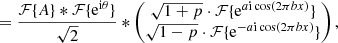
$$\begin{array}{c}\hfill \begin{array}{cc}\hfill E_{\mathrm{f}}& =\frac{\text{sinc}(f_x)\ast (\alpha +i\beta )}{\sqrt{2}}\ast \hfill \\ \hfill & \left(\begin{array}{c}\sqrt{1+p}[1+\sum _{n=1}^{\infty }\frac{{(i)}^n{a}^n}{n!}\mathcal{F}\{{cos}^n(2\pi bx)\}]\\ \sqrt{1-p}[1+\sum _{n=1}^{\infty }\frac{{(i)}^n{(-a)}^n}{n!}\mathcal{F}\{{cos}^n(2\pi bx)\}]\end{array}\right).\hfill \end{array}\end{array}$$(9)

Equation (9) shows that the VPSG creates an infinite number of speckles with decreasing brightness. For now, we assume that a ≪ 1 radian and expand Eq. (9) to first order (n = 1). Working out the terms in Eq. (9), we find:

$$\begin{array}{c}\hfill \begin{array}{cc}\hfill E_{\mathrm{f}}& =\frac{\alpha +i\beta }{\sqrt{2}}\ast \hfill \\ \hfill & \left(\begin{array}{c}\sqrt{1+p}[\text{sinc}(f_x)+\frac{\mathit{ai}}{2}(\text{sinc}(f_x-b)+\text{sinc}(f_x+b))]\\ \sqrt{1-p}[\text{sinc}(f_x)-\frac{\mathit{ai}}{2}(\text{sinc}(f_x-b)+\text{sinc}(f_x+b))]\end{array}\right).\hfill \end{array}\end{array}$$(10)

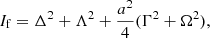
Rearranging in the real and imaginary terms, and computing the focal-plane intensity ($I_{\text{f}}=E_{\text{f}}\cdot E_{\text{f}}^{*}$) results in:

$$\begin{array}{c}\hfill I_{\mathrm{f}}=\underset{\mathrm{PSF}}{\underbrace{{\mathrm{\Delta }}^2+{\mathrm{\Lambda }}^2}}+\underset{\mathrm{speckle}\mathrm{grid}}{\underbrace{\frac{a^2}{4}({\mathrm{\Gamma }}^2+{\mathrm{\Omega }}^2)}}+\underset{\mathrm{cross}-\mathrm{talk}\mathrm{of}\mathrm{PSF}\mathrm{with}\mathrm{speckle}\mathrm{grid}}{\underbrace{ap(\mathrm{\Delta }\mathrm{\Gamma }+\mathrm{\Lambda }\mathrm{\Omega }).}}\end{array}$$(11)

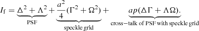
Greek symbols are used here to simplify the notation and denote the following terms:

$$\begin{array}{cc}\hfill \mathrm{\Delta }& =\text{sinc}(f_x)\ast \alpha \hfill \end{array}$$(12)

$$\begin{array}{cc}\hfill \mathrm{\Gamma }& =[\text{sinc}(f_x-b)+\text{sinc}(f_x+b)]\ast \beta \hfill \end{array}$$(13)

$$\begin{array}{cc}\hfill \mathrm{\Lambda }& =\text{sinc}(f_x)\ast \beta \hfill \end{array}$$(14)

$$\begin{array}{cc}\hfill \mathrm{\Omega }& =[\text{sinc}(f_x-b)+\text{sinc}(f_x+b)]\ast \alpha .\hfill \end{array}$$(15)

Equation (11) shows that the focal-plane intensity can be divided into three terms: the stellar PSF, the speckle grid, and the cross-talk between the speckle grid and the PSF. We find that the relative intensity of the speckle grid is given by I_s = a²/4. The performance of regular SGs is limited by the cross-talk term. For the VPSG, when p = 0 (i.e. with unpolarized light), the cross-talk term is eliminated and Eq. (11) reduces to:

$$\begin{array}{c}\hfill I_{\mathrm{f}}={\mathrm{\Delta }}^2+{\mathrm{\Lambda }}^2+\frac{a^2}{4}({\mathrm{\Gamma }}^2+{\mathrm{\Omega }}^2),\end{array}$$(16)

effectively making the VPSG incoherent with the PSF.

The remaining cross-talk that degrades the photometric and astrometric performance is the interference between the speckles themselves:

$$\begin{array}{c}\hfill \begin{array}{cc}\hfill {\mathrm{\Gamma }}^2+{\mathrm{\Omega }}^2=& \underset{\mathrm{speckle}1}{\underbrace{{(\text{sinc}(f_x-b)\ast \alpha )}^2+{(\text{sinc}(f_x-b)\ast \beta )}^2}}\hfill \\ \hfill & +\underset{\mathrm{speckle}2}{\underbrace{{(\text{sinc}(f_x+b)\ast \alpha )}^2+{(\text{sinc}(f_x+b)\ast \beta )}^2}}\hfill \\ \hfill & +\underset{\mathrm{cross}-\mathrm{talk}\mathrm{between}\mathrm{speckles}}{\underbrace{2(\text{sinc}(f_x-b)\ast \alpha ·\text{sinc}(f_x+b)\ast \alpha }}\hfill \\ \hfill & +\underset{\mathrm{cross}-\mathrm{talk}\mathrm{between}\mathrm{speckles}}{\underbrace{\text{sinc}(f_x-b)\ast \beta ·\text{sinc}(f_x+b)\ast \beta )).}}\hfill \end{array}\end{array}$$(17)

We have not found a method to mitigate this effect, and consider this cross-talk to be the fundamental limiting factor of the VSG. Its effect can be reduced by minimizing the number of speckles in the VSG and increasing their separation. This can be understood as follows: the distortion of an artificial speckle is determined by the relative strength of the combined electric field of the other artificial speckles (the distorting electric field) at its location, relative to its own electric field strength. If the distorting electric field becomes stronger, the cross-talk terms in Eq. (17) become more important and the artificial speckle is more distorted. If there are fewer artificial speckles in the VSG, the distorting electric field becomes weaker. Furthermore, as the electric field an artificial speckles scales with $f_x^{-1}$ (Eq. (6)), placing the artificial speckles further apart also reduces the distorting electric field.

We expanded Eq. (9) to first order and ignored higher order terms; we discuss their effects here. The higher order terms can be divided into two groups: the odd orders (n= odd) and the even orders (n= even). The amplitude of the higher order terms is given by (a)ⁿ. For the odd orders, n is odd, and therefore, when a flips its sign (a → −a), the higher orders also have a sign flip. Which means that all the odd orders become incoherent as the cross-talk term between the PSF and the speckle grid cancels when p = 0. For the even orders (n= even), a sign flip of a does not result in a sign flip of (a)ⁿ. This means that none of the even orders are incoherent as the cross-talk term does not cancel. As the even orders fall at other spatial locations and are much fainter than the first order speckles, the impact of the coherent even orders is minimal.

2.2. Vector amplitude speckle grid

Here we derive how the incoherency of the VASG arises. This derivation is very similar to what is presented in Sect. 2.1 and starts with the same assumptions. The VASG is implemented by a sine wave (with spatial frequency b) on the pupil amplitude, with opposite amplitude a for the two opposite polarization states:

$$\begin{array}{c}\hfill E_{\mathrm{p}}=\frac{A{\mathrm{e}}^{\mathrm{i}\theta }}{\sqrt{2}}\left(\begin{array}{c}\sqrt{1+p}[1+asin(2\pi bx)]\\ \sqrt{1-p}[1-asin(2\pi bx)]\end{array}\right).\end{array}$$(18)

We calculate the focal-plane electric field E_f by taking the Fourier transform (ℱ{⋅}) of E_p:

$$\begin{array}{cc}\hfill E_{\mathrm{f}}& =\mathcal{F}\{E_{\mathrm{p}}\}\hfill \end{array}$$(19)

$$\begin{array}{cc}& =\frac{\mathcal{F}\{A\}\ast \mathcal{F}\{e^{i\theta }\}}{\sqrt{2}}\ast \left(\begin{array}{c}\sqrt{1+p}[1+a\mathcal{F}\{sin(2\pi bx)\}]\\ \sqrt{1-p}[1-a\mathcal{F}\{sin(2\pi bx)\}]\end{array}\right).\hfill \end{array}$$(20)

Using Eq. (8) and working out the Fourier transforms of the terms in Eq. (20), we find:

$$\begin{array}{c}\hfill \begin{array}{cc}\hfill E_{\mathrm{f}}& =\frac{\alpha +i\beta }{\sqrt{2}}\ast \hfill \\ \hfill & \left(\begin{array}{c}\sqrt{1+p}[\text{sinc}(f_x)+\frac{\mathit{ai}}{2}(\text{sinc}(f_x-b)-\text{sinc}(f_x+b))]\\ \sqrt{1-p}[\text{sinc}(f_x)-\frac{\mathit{ai}}{2}(\text{sinc}(f_x-b)-\text{sinc}(f_x+b))]\end{array}\right).\hfill \end{array}\end{array}$$(21)

Rearranging this in its real and imaginary terms, and computing the focal-plane intensity ($I_{\text{f}}=E_{\text{f}}\cdot E_{\text{f}}^{*}$) results in:

$$\begin{array}{c}\hfill I_{\mathrm{f}}=\underset{\text{PSF}}{\underbrace{{\mathrm{\Delta }}^2+{\mathrm{\Lambda }}^2}}+\underset{\text{speckle grid}}{\underbrace{\frac{a^2}{4}({\mathrm{\Gamma }}^2+{\mathrm{\Omega }}^2)}}+\underset{\mathrm{cross}-\mathrm{talk}\mathrm{of}\mathrm{PSF}\mathrm{with}\mathrm{speckle}\mathrm{grid}}{\underbrace{ap(\mathrm{\Delta }\mathrm{\Gamma }+\mathrm{\Lambda }\mathrm{\Omega }).}}\end{array}$$(22)

As in Sect. 2.1, the Greek symbols denote the following terms:

$$\begin{array}{cc}\hfill \mathrm{\Delta }& =\text{sinc}(f_x)\ast \alpha \hfill \end{array}$$(23)

$$\begin{array}{cc}\hfill \mathrm{\Gamma }& =[\text{sinc}(f_x-b)-\text{sinc}(f_x+b)]\ast \beta \hfill \end{array}$$(24)

$$\begin{array}{cc}\hfill \mathrm{\Lambda }& =\text{sinc}(f_x)\ast \beta \hfill \end{array}$$(25)

$$\begin{array}{cc}\hfill \mathrm{\Omega }& =[\text{sinc}(f_x-b)-\text{sinc}(f_x+b)]\ast \alpha \hfill \end{array}$$(26)

In Eq. (22) we find again that the relative intensity of the speckle grid is given by I_s = a²/4, and that the VASG becomes incoherent when p = 0. As with the VPSG, the remaining cross-talk that degrades the photometric and astrometric performance is the interference between the speckles themselves. We also note that this implementation with a sine wave modulation of the VASG does not generate any higher order speckles. A VASG implementation comparable to the GPI amplitude grating (Wang et al. 2014) will introduce higher order speckles in a similar manner to the VPSG.

3. Simulations

3.1. Performance quantification

To validate the VSG concept and quantify the performance increase that VSGs could bring compared to regular SGs, we performed idealised numerical simulations. These are performed in Python using the HCIPy package¹ (Por et al. 2018), which supports polarization propagation with Jones calculus necessary for simulating VSGs. It is notoriously hard to realistically simulate high-contrast imaging observations as not all speckle noise sources are well understood (Guyon et al. 2019), thus making it hard to predict the on-sky performance of the VSG. Therefore, we decided to limit the scope of the simulations. We simulated a general HCI instrument with coronagraph and AO system at an 8 m class telescope with a clear aperture under various atmospheric conditions, and did not include any other noise sources (e.g. detector and photon noise, evolving non-common path aberrations). An overview of the simulation parameters is shown in Table 2. We only considered monochromatic images as we leave broadband effects for future work. The images are recorded at a wavelength of 1220 nm, which is at the centre of J-band, a scientifically interesting band for photometric variations of exoplanets (Kostov & Apai 2012). We considered three cases of atmospheric conditions, under which the current generation of HCI instruments regularly operate:

1. Good conditions with a seeing of 0.6″ and wind speed of 4.4 m s⁻¹.

2. Medium conditions with a seeing of 1″ and wind speed of 8.8 m s⁻¹.

3. Poor conditions with a seeing of 1.4″ and wind speed of 13.2 m s⁻¹.

These atmospheric conditions were simulated as an evolving turbulent wavefront assuming the “Frozen Flow” approximation with a von-karman power spectrum. The AO system that measures and corrects the atmospheric conditions consists of a noiseless wavefront sensor, and a deformable mirror with 40 × 40 actuators in a rectangular grid. The AO system runs at 2 kHz and has a three-frame lag between measurement and correction. The root mean square (rms) residual wavefront error after the AO system is respectively 44 nm, 70 nm, and 95 nm for the good, medium, and poor atmospheric conditions. Following the Maréchal approximation (Roberts et al. 2004), these residual wavefront errors correspond to Strehl ratios of 95%, 88%, and 79%, respectively (calculated at λ = 1220 nm). With this setup we only consider the speckle noise from the free atmosphere. As the decorrelation timescale for such speckles is on the order of ∼1 s (Macintosh et al. 2005), we limited the duration of the simulation to 1 s. For longer simulations, the background speckles would effectively become incoherent with the SGs. Focal-plane images were recorded at 2 kHz. The coronagraph in this setup is the Vector Vortex Coronagraph (VVC; Mawet et al. 2005) with an accompanying Lyot stop with a 95% diameter. The VVC is a focal-plane mask that removes starlight and operates on the vector state of light. The reason for implementing the VVC in this simulation is twofold: first, for a clear aperture, the performance of the VVC is close to that of the perfect coronagraph (Cavarroc et al. 2006), and second, as the VVC also operates on the vector state of light, we show that the performance of the VSG will not be affected by such optics. The SGs are placed at [ ± 25λ/D, ±25λ/D], which is well beyond the control radius of the AO system. The intensities of the SGs relative to the PSF core are 5 × 10⁻³, making them ∼150, 63, and 35 times brighter than the background speckle halo for the good, medium, and poor atmospheric conditions, respectively. We compare the phase speckle grid (PSG) and the amplitude speckle grid (ASG) to the VPSG and the VASG. We did not include any temporally modulated SGs because, when assuming an instantaneous modulation, their performance is equal to the VSG. The VPSG and VASG are implemented on the circular polarization state. The simulations were performed with the same wavefronts for all the SGs. We also performed the same simulations without a SG for accurate background estimation.

In Fig. 1 we show images of the SGs at a random iteration in the simulation for medium atmospheric conditions. The coronagraph and AO system removed the central stellar light and generated the dark hole, which is clearly visible. The idealistic AO system gives an optimistic contrast in the dark hole. Outside of the dark hole and control region, the speckle background is clearly visible. This background is generated by residual wavefront errors and evolves during the simulation. It will strongly interfere with the SGs, affecting their photometric and astrometric accuracy. The reference speckles of the SG are located in the corners of the images (±25 λ/D, ±25 λ/D). The VPSG and VASG are significantly less distorted and more similar to each other compared to the PSG and ASG. This shows the effect of the incoherency of the VSG. Zooming in on the lower left reference speckles as shown in Fig. 2 demonstrates this as well.

Fig. 1. Short-exposure images at a random iteration in the simulation with the medium atmospheric conditions (seeing of 1″ and wind speed of 8.8 m s−1). The dark hole in the center of the images is generated by the AO system and the Vector Vortex Coronagraph. The reference speckles are located in the corners of the image at [±25 λ/D, ±25 λ/D]. We note that the reference speckles generated by the VPSG and VASG are significantly less distorted and more similar to each other compared to the Phase and Amplitude Speckle Grids. The images show intensity normalized to the maximum of the star in logarithmic scale, and share the same color bar (shown at the right).

Fig. 2. Zoom onto the reference speckles in the lower left corner of the panels in Fig. 1. The VSGs are clearly less distorted compared to the regular SGs. The images show intensity normalized to the maximum of the star in logarithmic scale, and share the same color bar (shown at the right).

To quantify the performance increase offered by the VSGs, we calculate the rms photometric error and the rms astrometric error. These are calculated on the individual frames, and images that are averages of 5, 10, 50, and 100 frames to simulate longer exposure times. The photometric performance is calculated by carrying out the following steps:

1. Measure the photometry of the SG with an aperture with a diameter of 2.44 λ/D.

2. Measure the background by aperture photometry in the simulation without SG at the same positions.

3. Subtract the background estimate from the SG photometry.

4. Remove the general photometric fluctuations by dividing the SG photometry by the mean photometry of the four speckles.

5. Calculate the rms photometry error per speckle.

6. Determine the final rms photometric error by calculating the mean of the four speckles individual rms photometric errors.

The astrometric performance is calculated by carrying out the following steps:

1. Measure the position of the individual speckles by cross-correlation with an unaberrated PSF.

2. Calculate the distance between the speckles.

3. Calculate the rms of these distances over all images.

4. Calculate the mean rms astrometric error over all the distances, which gives the final rms astrometric error.

In Fig. 3 we plot the photometric and astrometric performance of the SGs as a function of the number of averaged frames (bin factor) and for the different atmospheric conditions. Figure 3 a shows that the VASG and the VPSG outperform the ASG and PSG in photometric error by a factor of ∼10–20 (depending on the bin factor and atmospheric conditions). The VASG and VPSG reach a ∼0.3–0.8% photometric error for individual frames, which drops to ∼0.2% when the bin factor increases. The ASG and PSG on the other hand start at ∼6–15% photometric error and decrease to ∼1.5–4%. Figure 3b also shows a performance increase for the astrometric performance. The VASG and VPSG improve the astrometric error by a factor of ∼3–5 with respect to the ASG and PSG. At a bin factor of one, the VSGs reach an astrometric error of ∼3−10 × 10⁻³λ/D, and slightly improve for a bin factor of 100. The ASG and PSG start at ∼1.5−6 × 10⁻²λ/D and improve to ∼7−16 × 10⁻³λ/D. These results clearly demonstrate that VSGs greatly improve the photometric and astrometric precision with respect to their non-vector counterparts.

Fig. 3. Photometric and astrometric performance of the SGs as a function of the number of frames averaged, and for various atmospheric conditions (Table 2). Panel a: rms relative photometric error. Panel b: rms astrometric error.

For poorer seeing conditions, the performance of all SGs decreases. For the ASG and PSG, this is due to the increased speckle background halo that interferes with the SG (Eq. (11)), while for the VSGs this is due to the increased cross-talk between the reference speckles (Eq. (17)). When the wind speed increases, the performance of the SGs increases more rapidly with bin factor. This is because the decorrelation timescale of background speckles scales with the inverse of the windspeed (Macintosh et al. 2005). Therefore, for higher wind speeds, the interference between the background speckles and SGs will decrease with increasing bin factor, improving their performance.

3.2. Degree of polarization effects

As discussed in Sect. 2, the incoherency of the VSGs depends on the degree of polarization (p; Eq. (2)) of the light passing through the VSG (specifically the polarization state on which the VSG operates). As starlight is generally unpolarized to a very high degree (e.g. the integrated p of the Sun is < 10⁻⁶; Kemp et al. 1987), we are mainly concerned with polarization introduced by the telescope and instrument. For VLT/SPHERE, the linear p has been measured to be on the order of a few percent (Van Holstein et al. 2020) and the circular p is expected to be even lower. To study the effect of p, we repeat the simulations of Fig. 3 with the medium atmospheric conditions for the VSGs but with increasing levels of p. The simulations are performed with the same wavefronts as in Fig. 3. Therefore, for p = 0, we expect exactly the same results, while for p = 1 the performance of the VSGs should reduce to that of the ASG and PSG. Figure 4a shows the photometric performance and Fig. 4b the astrometric performance. Both figures indeed show that the performance of the VASG and VPSG degrade to that of the ASG and PSG when p = 1, and are optimal for p = 0. They also show that up to a p of 0.05 there is barely a performance degradation. The performance degrades close to linearly as a function of p, which is what we expect from Eq. (11).

Fig. 4. Photometric and astrometric performance of the VPSG and VASG as a function of the number of frames averaged and various degrees of polarization (p) under medium atmospheric conditions (Table 2). Panel a: rms relative photometric error. Panel b: rms astrometric error.

4. Implementation of vector speckle grid

Now that we have demonstrated that VSGs can drastically improve the photometric and astrometric performance, we discuss how VSGs can be implemented in a HCI system. We focus on the VPSG as we have not found a straightforward implementation of the VASG.

The most attractive solution for the implementation of the VPSG is the geometric phase (Pancharatnam 1956; Berry 1987), which applies the required phase to the opposite circular polarization states. The geometric phase is introduced when the fast-axis angle of a half-wave retarder is spatially varying. The phase that is induced is twice the fast-axis angle, and is opposite for the opposite circular polarization states. Due to its geometric origin, the geometric phase is completely achromatic. However, the efficiency with which the phase is transferred to the light depends on retardance offsets from half wave. Increasing the retardance offset decreases the amount of light that acquires the desired phase. The VPSGs simulated in Sect. 3 are implemented by geometric phase.

Half-wave retarders with a spatially varying fast-axis angle can be constructed in various ways. For example, metamaterials have been used to induce geometric phase, but their efficiency is generally low (Mueller et al. 2017). The most mature and promising is liquid-crystal technology (Escuti et al. 2016). By a direct-write system, the desired fast-axis angle can be printed into a liquid-crystal photo-alignment layer that that has been deposited on a substrate (Miskiewicz & Escuti 2014). To achromatise the half-wave retarder, several layers of carefully designed, self-aligning birefringent liquid crystals can be deposited on top of the initial layer (Komanduri et al. 2013). In astronomy, there have already been several successful (broadband) implementations of this technology: in coronagraphy (Mawet et al. 2009; Snik et al. 2012), polarimetry (Tinyanont et al. 2018; Snik et al. 2019), wavefront sensing (Haffert 2016; Doelman et al. 2019), and interferometry (Doelman et al. 2018).

The major drawback of liquid-crystal technology is when there are retardance offsets from half-wave, as the efficiency with which the light accumulates the desired phase decreases. The light that does not acquire the desired phase will form an on-axis PSF, which is regularly referred to as the leakage. In coronagraphy, the leakage severely limits the coronagraphic performance of the liquid-crystal optic (Bos et al. 2018; Doelman et al. 2020). However, for the VSG the impact is much less severe, because the leakage will overlap with the stellar PSF and therefore be occulted by the coronagraph. The relative intensity of the VSG will be affected, but this effect will be relatively small as I_s ∝ (1 − L) (Bos et al. 2019), with L the leakage strength. The leakage strength is generally on the order of ∼2 × 10⁻² (Doelman et al. 2017) for broadband devices.

5. Discussion and conclusion

Here, we show that by applying opposite modulation on opposite polarization states in the pupil-plane amplitude or phase, a speckle grid in the focal plane is generated that can be used as a photometric and astrometric reference. We refer to this as the Vector Speckle Grid (VSG). In this implementation, the speckle grid will not interfere with the central stellar PSF and will therefore be effectively incoherent. This greatly decreases the photometric and astrometric errors when the PSF is distorted by aberrations. Furthermore, we identified that the remaining limiting factor is the cross-talk between the speckles in the grid itself. This can be mitigated by increasing the separation between the speckles.

We performed simulations with various atmospheric conditions to quantify the performance increase with respect to regular SGs. We find that for the conditions simulated, the VSGs improve the photometric and astrometric errors by a factor of ∼20 and ∼5, respectively, reaching a ∼0.3–0.8% photometric and a ∼3−10 × 10⁻³λ/D astrometric error on short exposure images. We note that the performance increase depends on the brightness difference between the speckle and the residual speckle background. When the brightness difference increases, the performance increase is more moderate. If the speckles are dimmer, the performance increase is higher. We also investigated the effects of partially polarized light on the performance of the VSGs. The simulations showed that when the degree of polarization was below 5%, the performance was barely affected. The polarization signal introduced by the telescope and instrument is on this level or less, and therefore not relevant. We note that it is hard to predict what the on-sky performance will be as it is notoriously difficult to capture all relevant effects in simulation (Guyon et al. 2019). Therefore, these results are an indication of the performance increase that the VSGs could bring. We also note that the performance of the ASG and PSG reported in these simulations is better than what has been reported on-sky, while the duration of the simulations is much shorter than the actual observations. This is because these simulations only consider the effects of AO-corrected atmospheric wavefront errors, while observations are also affected by noise processes that generate background speckles with much longer decorrelation timescales. The VSG would also be incoherent to these background speckle noise sources.

We identified that the most attractive implementation of VSGs would be a Vector Phase Speckle Grid (VPSG) by the geometric phase. Liquid-crystal technology allows for a broadband half-wave retarder with a varying fast-axis angle that will induce the geometric phase on the light. This has the major advantage that the VPSG can be implemented as a one pupil-plane optic.

Implementing the VPSG by liquid-crystal technology has the following advantages: it achieves instantaneous incoherency, it is a static component and therefore easy to calibrate, the artificial speckles can be positioned anywhere in the focal plane, the geometric phase is achromatic and therefore the speckles have a constant brightness with wavelength. Another advantage, not discussed in this paper, is that the VPSG could be multiplexed with holograms for wavefront sensing (Wilby et al. 2017). The main disadvantage of the VPSG is that the position of the speckles is fixed, making accurate background estimates more difficult, and decreasing the flexibility of speckle grid positioning.

To conclude, the VSG has proven to be a promising method for generating speckle grids as photometric and astrometric references. We show that the VSG reaches a satisfactory performance in simulation, and the next steps will be an investigation of broadband effects, a lab demonstration, and subsequent on-sky tests. The VSG could be part of the future upgrades of SPHERE and GPI (Beuzit et al. 2018; Chilcote et al. 2018).

Acknowledgments

The author thanks the referee for comments on the manuscript that improved this work. The author also thanks F. Snik for his comments on the manuscript. The research of S.P. Bos leading to these results has received funding from the European Research Council under ERC Starting Grant agreement 678194 (FALCONER). This research made use of HCIPy, an open-source object-oriented framework written in Python for performing end-to-end simulations of high-contrast imaging instruments (Por et al. 2018). This research used the following Python libraries: Scipy (Jones et al. 2014), Numpy (Walt et al. 2011), and Matplotlib (Hunter 2007).

References

All Tables

All Figures

Fig. 1. Short-exposure images at a random iteration in the simulation with the medium atmospheric conditions (seeing of 1″ and wind speed of 8.8 m s−1). The dark hole in the center of the images is generated by the AO system and the Vector Vortex Coronagraph. The reference speckles are located in the corners of the image at [±25 λ/D, ±25 λ/D]. We note that the reference speckles generated by the VPSG and VASG are significantly less distorted and more similar to each other compared to the Phase and Amplitude Speckle Grids. The images show intensity normalized to the maximum of the star in logarithmic scale, and share the same color bar (shown at the right).

In the text

	Fig. 2. Zoom onto the reference speckles in the lower left corner of the panels in Fig. 1. The VSGs are clearly less distorted compared to the regular SGs. The images show intensity normalized to the maximum of the star in logarithmic scale, and share the same color bar (shown at the right).
In the text

	Fig. 3. Photometric and astrometric performance of the SGs as a function of the number of frames averaged, and for various atmospheric conditions (Table 2). Panel a: rms relative photometric error. Panel b: rms astrometric error.
In the text

	Fig. 4. Photometric and astrometric performance of the VPSG and VASG as a function of the number of frames averaged and various degrees of polarization (p) under medium atmospheric conditions (Table 2). Panel a: rms relative photometric error. Panel b: rms astrometric error.
In the text

References

- Apai, D., Kasper, M., Skemer, A., et al. 2016, ApJ, 820, 40 [NASA ADS] [CrossRef] [Google Scholar]
- Berry, M. V. 1987, J. Mod. Opt., 34, 1401 [NASA ADS] [CrossRef] [Google Scholar]
- Beuzit, J.-L., Mouillet, D., Fusco, T., et al. 2018, Adaptive Optics Systems VI, Int. Soc. Opt. Photonics, 10703, 107031P [Google Scholar]
- Beuzit, J.-L., Vigan, A., Mouillet, D., et al. 2019, A&A, 631, A155 [NASA ADS] [CrossRef] [EDP Sciences] [Google Scholar]
- Bos, S. P., Doelman, D. S., de Boer, J., et al. 2018, in Advances in Optical and Mechanical Technologies for Telescopes and Instrumentation III, Int. Soc. Opt. Photonics, 10706, 107065M [Google Scholar]
- Bos, S. P., Doelman, D. S., Lozi, J., et al. 2019, A&A, 632, A48 [NASA ADS] [CrossRef] [EDP Sciences] [Google Scholar]
- Cavarroc, C., Boccaletti, A., Baudoz, P., Fusco, T., & Rouan, D. 2006, A&A, 447, 397 [NASA ADS] [CrossRef] [EDP Sciences] [Google Scholar]
- Chilcote, J. K., Bailey, V. P., De Rosa, R., et al. 2018, in Ground-based and Airborne Instrumentation for Astronomy VII, Int. Soc. Opt. Photonics, 10702, 1070244 [Google Scholar]
- Doelman, D. S., Snik, F., Warriner, N. Z., & Escuti, M. J. 2017, in Techniques and Instrumentation for Detection of Exoplanets VIII, Int. Soc. Opt. Photonics, 10400, 104000U [Google Scholar]
- Doelman, D. S., Tuthill, P., Norris, B., et al. 2018, in Optical and Infrared Interferometry and Imaging VI, Int. Soc. Opt. Photonics, 10701, 107010T [Google Scholar]
- Doelman, D. S., Auer, F. F., Escuti, M. J., & Snik, F. 2019, Opt. Lett., 44, 17 [NASA ADS] [CrossRef] [Google Scholar]
- Doelman, D. S., Por, E. H., Ruane, G., Escuti, M. J., & Snik, F. 2020, PASP, 132, 045002 [CrossRef] [Google Scholar]
- Escuti, M. J., Kim, J., & Kudenov, M. W. 2016, Opt. Photonics News, 27, 22 [CrossRef] [Google Scholar]
- Fitzgerald, M. P., & Graham, J. R. 2006, ApJ, 637, 541 [NASA ADS] [CrossRef] [Google Scholar]
- Guyon, O., Bottom, M., Chun, M., et al. 2019, BAAS, 51, 203 [Google Scholar]
- Haffert, S. 2016, Opt. Exp., 24, 18986 [CrossRef] [Google Scholar]
- Hinkley, S., Oppenheimer, B. R., Soummer, R., et al. 2007, ApJ, 654, 633 [NASA ADS] [CrossRef] [Google Scholar]
- Hunter, J. D. 2007, Comput. Sci. Eng., 9, 90 [NASA ADS] [CrossRef] [Google Scholar]
- Jones, E., Oliphant, T., & Peterson, P. 2014, SciPy: Open Source Scientific Tools for Python [Google Scholar]
- Jovanovic, N., Martinache, F., Guyon, O., et al. 2015a, PASP, 127, 890 [NASA ADS] [CrossRef] [Google Scholar]
- Jovanovic, N., Guyon, O., Martinache, F., et al. 2015b, ApJ, 813, L24 [NASA ADS] [CrossRef] [Google Scholar]
- Kemp, J. C., Henson, G., Steiner, C., & Powell, E. 1987, Nature, 326, 270 [NASA ADS] [CrossRef] [Google Scholar]
- Komanduri, R. K., Lawler, K. F., & Escuti, M. J. 2013, Opt. Express, 21, 404 [NASA ADS] [CrossRef] [Google Scholar]
- Kostov, V., & Apai, D. 2012, ApJ, 762, 47 [CrossRef] [Google Scholar]
- Langlois, M., Vigan, A., Moutou, C., et al. 2013, Proc. Third AO4ELT Conf., 63 [Google Scholar]
- Macintosh, B., Poyneer, L., Sivaramakrishnan, A., & Marois, C. 2005, in Astronomical Adaptive Optics Systems and Applications II, Int. Soc. Opt. Photonics, 5903, 59030J [CrossRef] [Google Scholar]
- Macintosh, B., Graham, J. R., Ingraham, P., et al. 2014, Proc. Nat. Acad. Sci., 111, 12661 [Google Scholar]
- Marois, C., Lafreniere, D., Macintosh, B., & Doyon, R. 2006, ApJ, 647, 612 [NASA ADS] [CrossRef] [Google Scholar]
- Martinez, P., Loose, C., Carpentier, E. A., & Kasper, M. 2012, A&A, 541, A136 [NASA ADS] [CrossRef] [EDP Sciences] [Google Scholar]
- Martinez, P., Kasper, M., Costille, A., et al. 2013, A&A, 554, A41 [NASA ADS] [CrossRef] [EDP Sciences] [Google Scholar]
- Mawet, D., Riaud, P., Absil, O., & Surdej, J. 2005, ApJ, 633, 1191 [NASA ADS] [CrossRef] [Google Scholar]
- Mawet, D., Serabyn, E., Liewer, K., et al. 2009, Opt. Exp., 17, 1902 [NASA ADS] [CrossRef] [Google Scholar]
- Milli, J., Banas, T., Mouillet, D., et al. 2016, in Adaptive Optics Systems V, Int. Soc. Opt. Photonics, 9909, 99094Z [CrossRef] [Google Scholar]
- Miskiewicz, M. N., & Escuti, M. J. 2014, Opt. Exp., 22, 12691 [NASA ADS] [CrossRef] [Google Scholar]
- Mueller, J. B., Rubin, N. A., Devlin, R. C., Groever, B., & Capasso, F. 2017, Phys. Rev. Lett., 118, 113901 [CrossRef] [Google Scholar]
- Pancharatnam, S. 1956, Proc. Indian Acad. Sci.-Sect. A, 44, 398 [Google Scholar]
- Por, E. H., Haffert, S. Y., Radhakrishnan, V. M., et al. 2018, in Adaptive Optics Systems VI, Proc. SPIE, 10703 [Google Scholar]
- Roberts, L. C. J., Perrin, M. D., Marchis, F., et al. 2004, in Advancements in Adaptive Optics, Int. Soc. Opt. Photonics, 5490, 504 [NASA ADS] [CrossRef] [Google Scholar]
- Sivaramakrishnan, A., & Oppenheimer, B. R. 2006, ApJ, 647, 620 [NASA ADS] [CrossRef] [Google Scholar]
- Sivaramakrishnan, A., Lloyd, J. P., Hodge, P. E., & Macintosh, B. A. 2002, ApJ, 581, L59 [NASA ADS] [CrossRef] [Google Scholar]
- Snik, F., Otten, G., Kenworthy, M., et al. 2012, in Modern Technologies in Space-and Ground-based Telescopes and Instrumentation II, Int. Soc. Opt. Photonics, 8450, 84500M [CrossRef] [Google Scholar]
- Snik, F., Keller, C. U., Doelman, D. S., et al. 2019, in Polarization Science and Remote Sensing IX, Int. Soc. Opt. Photonics, 11132, 111320A [Google Scholar]
- Soummer, R., Ferrari, A., Aime, C., & Jolissaint, L. 2007, ApJ, 669, 642 [NASA ADS] [CrossRef] [Google Scholar]
- Tinyanont, S., Millar-Blanchaer, M. A., Nilsson, R., et al. 2018, PASP, 131, 025001 [CrossRef] [Google Scholar]
- Van Holstein, R. G., Girard, J. H., De Boer, J., et al. 2020, A&A, 633, A64 [NASA ADS] [CrossRef] [EDP Sciences] [Google Scholar]
- Walt, S., Colbert, S. C., & Varoquaux, G. 2011, Comput. Sci. Eng., 13, 22 [CrossRef] [Google Scholar]
- Wang, J. J., Rajan, A., Graham, J. R., et al. 2014, in Ground-based and Airborne Instrumentation for Astronomy V, Int. Soc. Opt. Photonics, 9147, 914755 [Google Scholar]
- Wang, J. J., Graham, J. R., Pueyo, L., et al. 2016, AJ, 152, 97 [NASA ADS] [CrossRef] [Google Scholar]
- Wilby, M. J., Keller, C. U., Snik, F., Korkiakoski, V., & Pietrow, A. G. 2017, A&A, 597, A112 [NASA ADS] [CrossRef] [EDP Sciences] [Google Scholar]
- Zhou, Y., Apai, D., Schneider, G. H., Marley, M. S., & Showman, A. P. 2016, ApJ, 818, 176 [NASA ADS] [CrossRef] [Google Scholar]