| Issue |
A&A
Volume 638, June 2020
|
|
|---|---|---|
| Article Number | A30 | |
| Number of page(s) | 7 | |
| Section | Stellar structure and evolution | |
| DOI | https://doi.org/10.1051/0004-6361/202037743 | |
| Published online | 05 June 2020 | |
On the formation of hydrogen-deficient low-mass white dwarfs
1
Instituto de Astrofísica de La Plata, CONICET–UNLP, La Plata, Argentina
2
Facultad de Ciencias Astronómicas y Geofísicas, UNLP, La Plata, Argentina
e-mail: tbattich@fcaglp.unlp.edu.ar
Received:
14
February
2020
Accepted:
28
March
2020
Context. Two of the possible channels for the formation of low-mass (M⋆ ≲ 0.5 M⊙) hydrogen-deficient white dwarfs are the occurrence of a very-late thermal pulse after the asymptotic giant-branch phase or a late helium-flash onset in an almost stripped core of a red giant star.
Aims. We aim to asses the potential of asteroseismology to distinguish between the hot flasher and the very-late thermal pulse scenarios for the formation of low-mass hydrogen-deficient white dwarfs.
Methods. We computed the evolution of low-mass hydrogen-deficient white dwarfs from the zero-age main sequence in the context of the two evolutionary scenarios. We explore the pulsation properties of the resulting models for effective temperatures characterizing the instability strip of pulsating helium-rich white dwarfs.
Results. We find that there are significant differences in the periods and in the period spacings associated with low radial-order (k ≲ 10) gravity modes for white-dwarf models evolving within the instability strip of the hydrogen-deficient white dwarfs.
Conclusions. The measurement of the period spacings for pulsation modes with periods shorter than ∼500 s may be used to distinguish between the two scenarios. Moreover, period-to-period asteroseismic fits of low-mass pulsating hydrogen-deficient white dwarfs can help to determine their evolutionary history.
Key words: white dwarfs / asteroseismology / stars: evolution / stars: interiors / stars: oscillations / stars: low-mass
© ESO 2020
1. Introduction
White dwarf (WD) stars are the final stage in the life of the vast bulk of stars. Among the WDs, a great majority (∼80%) present hydrogen (H)-rich atmospheres (DA WDs). However, there is a significant percentage of WDs (∼20%) with H-deficient surfaces. H-deficient WDs exhibit a variety of spectral classes. Among them, there are the helium (He)-rich DO WDs (with effective temperatures, Teff, in the range of 45 000 K ≲ Teff ≲ 200 000 K), the He-rich DB WDs (11 000 K ≲ Teff ≲ 45 000 K, with only few stars found in the range of 30 000 K ≲ Teff ≲ 45 000 K), and WDs with mainly carbon (C) or oxygen (O) in their spectra. The formation channel of these H-deficient WDs has long been a matter of study (see, for instance, Renzini et al. 1979, 1981; Schoenberner 1979; Iben et al. 1983 for earlier discussions on this matter). As the population of H-deficient WDs presents a variety of spectral types, among other particularities, it may be fed by different formation channels (Althaus et al. 2010). In particular, DO and DB WDs are believed to be mostly the progeny of PG1159 stars, which are hot C-, O- and He-rich WDs and pre-WDs. These stars, in turn, are expected to form via the very-late thermal-pulse scenario (VLTP; Miller Bertolami et al. 2006).
In the VLTP scenario, a post-AGB star experiences a final thermal pulse when the H-burning shell is almost extinct. Therefore, due to a low entropy barrier in this nearly extinct H-burning shell (see Iben 1976), convective processes carry H to the hot He-burning shell. As a consequence, all or almost all of the H is burned. As diffusion processes take place, a PG1159 star would evolve to a DO WD first, and to a DB WD later (Althaus et al. 2005). DO WDs could also be the descendants of low-mass H-deficient supergiant R Corona Borealis stars (RCrBs) – possibly linked to the O(He) stars – and the hotter extreme-He stars (EHe) or also the descendants of He-rich hot subdwarf stars (He-sdOs; Reindl et al. 2014a). A possible scenario for these types of stars is the merger of two WDs (Webbink 1984). The merger of a C-O core WD with a He-core WD would produce an RCrB star or an EHe star (Saio & Jeffery 2002; Longland et al. 2011; Jeffery et al. 2011; Lauer et al. 2019), meanwhile, the merger of two He-core WDs would produce a He-sdO (Zhang & Jeffery 2012; Schwab 2018). However, if the mass of the He-sdO is M⋆ ≲ 0.5 M⊙, it can also be formed via a late hot-flasher scenario with a deep-mixing episode (as classified by Lanz et al. 2004, see also Castellani & Castellani 1993; Brown et al. 2001; Cassisi et al. 2003; Miller Bertolami et al. 2008). This scenario is somehow similar to the VLTP, but instead of a late thermal pulse, what happens is a late onset of He-burning in the degenerate core of a low-mass star that has lost almost all, but not all, of its H-rich envelope (having a ∼1–5 10−4 M⊙ envelope mass). In this scenario, the He flash occurs when the star has a H-envelope mass that is too low to sustain a H-burning shell. Therefore, convection processes also carry H into the He-burning region where it is burned, leading to a H-deficient He-rich star. For this scenario to take place, the star needs to lose a significant amount of mass before the onset of He flash in the red giant branch. The mass loss can occur due to the presence of a companion star, both via mass transfer due to stable Roche lobe overflow or mass ejection in a common envelope phase (Paczynski et al. 1976; Han et al. 2003). Also, enhanced winds in the red giant branch due, for example, to rotation or enhanced initial He-compositions could lead to a significant envelope-mass loss (Sweigart 1997; Villanova et al. 2012; Tailo et al. 2015; Althaus et al. 2017). Hereinafter, we call this scenario the very-late hot-flasher (VLHF) scenario. The outcome of the VLHF scenario would be a star with a mass that is necessarily close to the mass required for the onset of He burning in a degenerate He core, that is, of about 0.45–0.49 M⊙ depending on metallicity and He-abundance. In summary, a low-mass (≲0.5 M⊙) H-deficient He-rich WD can either come from a VLTP of a low-mass star, a VLHF scenario, or a merger of two low-mass He-core WDs. Now, the question arises as to whether there are H-deficient He-rich WDs with such masses.
Historically, DB WDs were found to have a mass distribution with a mean mass similar to the one of DA WDs (∼0.6 M⊙), but without a significant spread to lower masses (Shipman 1979; Oke et al. 1984; Beauchamp et al. 1996; Bergeron et al. 2001, 2011; Voss et al. 2007). However, some DB WDs in the range of 0.4–0.5 M⊙ were found by different authors (see, e.g., Koester & Kepler 2015 from a pre-Gaia era). With the recent measurements of trigonometric parallaxes by Gaia, new mass distributions for WDs were derived in magnitude and volume-limited samples, for both H-rich and H-deficient WDs, using both photometric and spectroscopic techniques (Ourique et al. 2019; Genest-Beaulieu & Bergeron 2019a,b; Tremblay et al. 2019; Gentile Fusillo et al. 2019; Bergeron et al. 2019; Kepler et al. 2019). The most recent work for the case of He-rich WDs was carried out by Genest-Beaulieu & Bergeron (2019b). Regardless of the technique used, these authors found DB stars that appear to have masses below 0.5 M⊙ and even below 0.4 M⊙. They argue that these stars are most likely double degenerate binaries (DB+DB) that are not resolved, and therefore, they appear to have a large radius and hence a small mass. If this is not the case for all of them, however, they should have been formed through one of the scenarios mentioned above. Also, Reindl et al. (2014b) derived masses for a sample of DO WDs and found that some of them have masses below 0.5 M⊙. These authors argue that about 13% of the DO WDs may be the descendants of extreme horizontal branch (EHB) stars (i.e., He-sdO/B stars). All in all, the evolutionary history of DO and DB WDs is not completely clear. In particular, for DB/DO WDs with masses ≲0.5 M⊙, a VLHF scenario for their formation is also a possibility.
In this work, we aim to explore the differences in the evolutionary and pulsational properties of H-deficient low-mass WDs resulting from the VLTP and the VLHF scenarios, leaving the merger scenario for a future work. In order to do this, we take advantage of the fact that DB WDs are found to pulsate in the temperature range of 22 000 K < Teff < 30 000 K (Córsico et al. 2019). They are called DBV or V777 Her variable stars. Asteroseismology is a powerful tool to explore the internal chemical stratification of stars (Fontaine & Brassard 2008; Winget & Kepler 2008; Althaus et al. 2010; Córsico et al. 2019). The different physical processes taking place in the interior of stars that experience a VLTP or a VLHF would lead to different chemical profiles in the interior of the resultant low-mass WDs. These differences could have a distinct impact on the pulsational properties of the WDs. For instance, De Gerónimo et al. (2017) found differences in the period spectrum between DA WDs whose progenitors experienced thermal pulses and those DA WDs whose progenitors avoided the thermally pulsing phase. Motivated by this, we compare the pulsational properties of DB WDs models that come from these two scenarios (VLTP and the VLHF), with the aim of assessing the potential of asteroseismology to distinguish between those scenarios. Finally, there exist in the literature detailed WD models evolved from PG1159 stars within the VLTP scenario (Althaus et al. 2005; Miller Bertolami et al. 2006); however, detailed models of WDs coming from He-sdO stars are lacking. We present here for the first time detailed WD models that come from He-sdO star models, within the VLHF scenario.
The paper is organized as follows. In Sect. 2 we introduce the evolutionary sequences for both the VLTP and the VLHF scenarios. In Sect. 3 we present the pulsational properties of WD models resulting from both scenarios and discuss their differences. In Sect. 4 we provide a brief summary and present our conclusions.
2. Evolutionary sequences
For all the evolutionary calculations presented in this work, we used the LPCODE stellar evolution code (Althaus et al. 2005). The most recent updates to the code can be found in Miller Bertolami (2016). In Fig. 1 we plotted the Hertzsprung-Russell diagrams for both the VLTP and the VLHF sequences. In both sequences, we marked the locus of the maximum CNO-luminosity of the H flash with a star symbol. The stellar masses predicted by the hot-flasher scenario depend on the metallicity and range from approximately 0.455 M⊙ for Z = 0.02 to 0.485 M⊙ for Z = 0.001 (Miller Bertolami et al. 2008; Battich et al. 2018). For this work, we selected a sequence of 0.46 M⊙ with an initial metallicity and He abundance of Z = 0.02 and Y = 0.285. This sequence was extracted from those calculated in the work of Battich et al. (2018), and it experiences a deep-mixing scenario (Lanz et al. 2004) where almost all the H is burned. We evolved this sequence to the WD regime. The VLTP sequence was computed from the ZAMS with the same initial metallicity and He abundance as the VLHF sequence as well as an initial mass of 1 M⊙. In the AGB phase, we artificially removed mass of the star until the stellar mass was reduced to 0.5 M⊙, and we continued the remnant evolution along two thermal pulses, forcing the last one to be a VLTP. The VLTP was followed by the corresponding H burning. Before the WD stage was reached, we relaxed the mass of the star to 0.46 M⊙ in order to get rid of possible differences in the periods arising from differences in the mass of the models coming from the VLTP and the VLHF scenarios. For both sequences, we used a MLT parameter of αMLT = 1.822, which corresponds to the calibration of the solar model for the LPCODE (see Miller Bertolami 2016), and overshooting in the central He-burning phase to an extent of ∼0.2 the pressure scale height. The mass of the remaining H after the H flash was around MH = 10−7 M⊙ in both cases. For the VLHF this value drops below 10−10 M⊙ after the He subflashes. The exact value of the total amount of H that is burned in the H flash in both the VLTP and the VLHF scenarios depends on the details of convection and convective-border mixing processes. Since determining the amount of convective-border mixing that is needed in order to obtain a DB WD is beyond the scope of this work, we artificially removed the remaining H after the H flash in each case.
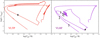 |
Fig. 1. Hertzsprung-Russell diagram for the VLTP scenario (left) and the VLHF scenario (right) computed from the main sequence to the WD stage. In both panels, the star symbol marks the model where the maximum CNO-luminosity of the H flash occurs. In the right panel, we show the location of the models of Fig. 2 (a, b, c, and d), and the model of the right panel of Fig. 3 (e). |
The evolution of PG1159 stars to the WD stage within the VLTP scenario is well documented (Althaus et al. 2005; Miller Bertolami et al. 2006). This is not the case for the evolution of He-sdOB stars to the WD stage within the VLHF scenario. We, therefore, show in Fig. 2 the evolution of the chemical profile from the end of the central He-burning phase (panel a) to the WD stage (panel d). We show, in Fig. 1, the location of these models in the Hertzsprung-Russell diagram. In panel a, we can see the O-rich core up to mr ≃ 0.15. At this point, the central He-burning has ceased, but there is still He-burning in the layer between mr = 0.15 and 0.25. In panels b and c, we see how the He remaining in this layer is burned into C and O. In panel d, He-burning has finished, and the C/O core has settled to its final shape, as diffusion processes do not significantly change the chemical structure at the high temperatures of the core. This model is already a WD model of Teff = 65800 K. Later, the model cools down to the DB WDs instability strip. In this cooling process, diffusion produces a pure He envelope as can be seen in the right panel of Fig. 3, where we plotted the WD model at Teff = 30 000 K. The locus of this model in the Hertzsprung-Russell diagram is marked with an e in Fig. 1.
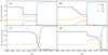 |
Fig. 2. Oxygen (O), carbon (C), and helium (He) profiles of the models highlighted in Fig. 1 with letters a, b, c, and d. |
We now compare the WD models coming from the VLTP and VLHF scenarios. In Fig. 3 we plotted the chemical profiles of the WDs models that come from both the VLTP and the VLHF for Teff = 30 000 K, which corresponds to the blue edge of the instability strip of the DBVs. In both evolutionary scenarios, the star evolves to a H-deficient WD, but the differences in the evolutionary history of both remnants are translated into different features in the chemical profiles. In the VLTP case, since thermal pulses have taken place, there are several changes in the slope of C and O profiles in the core. In the VLHF case, as no thermal pulse has taken place, the C/O profile has a simpler structure. Also, due to thermal pulses, in the VLTP model remains an intershell where a significant amount of He, C, and O coexists. Meanwhile, in the VLHF model, this feature is not present. Only a small amount of C up to q = 5 and O up to q = 1.5 can be seen as a consequence of the core He flash. In addition, in the VLTP model, where He-layer burning has been active for a longer time than in the VLHF, the C/O core is more massive, being the C/He transition at q ≃ 1.3, which is in contrast with the value of q = 1 for the C/He transition in the VLHF model.
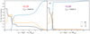 |
Fig. 3. Oxygen (O), carbon (C), and helium (He) profiles of WD models coming from a VLTP (left) and a VLHF (right) at Teff = 30 000 K. |
3. Pulsational properties
We calculated nonradial adiabatic gravity (g) modes for all the WDs models with effective temperatures in the range of the instability strip of DBVs (22 000 ≲ Teff ≲ 32 000 K) for both the VLTP and VLHF scenarios. The periods observed in DB WDs range from approximately 120 s to 1100 s (Córsico et al. 2019). We calculated periods from 100 s to 2500 s for harmonic degree ℓ = 1 and 2, thus covering the range of observed periods. All the calculations were made with the stellar-pulsation code LP-PUL (Córsico et al. 2006). We focus on pulsational results with ℓ = 1 only because they qualitatively do not differ from the results for ℓ = 2. In Fig. 4 we show the logarithm of the squared Brunt-Väisälä and Lamb frequencies, plotted together with the chemical profiles for the same models of Fig. 3. The Brunt-Väisälä frequency (N) is strongly dependent on the chemical structure. Any chemical interface imprints a bump in N. For this reason, for a WD that comes from a VLTP, N has a more complicated structure than for a WD coming from a VLHF. In particular, we can see a bump at q ∼ 1.7 in the VLTP model that is not present in the VLHF model because this last one lacks the intershell where a significant amount of O, C, and He coexists. Also, the bump corresponding to the C-He transition at q = 1 for the VLHF is more pronounced than the bump in the VLTP model. This is because the C-He transition in the VLHF profile is very well defined and steeper than in the VLTP case, making the mode-trapping cavity of the core more noticeable in the VLHF profile. This cavity is also smaller than in the VLTP case, where the transition is at q ≃ 1.3. Therefore, we see differences in the Brunt-Väisälä frequency that arise from different features in the chemical profiles of the models. DBV WDs exhibit periods associated with g modes. The properties of the g-mode spectrum are strongly dependent on the Brunt-Väisälä frequency. Therefore, we expect that the period spectrum of the DB WDs is affected by the differences in the Brunt-Väisälä frequencies of both models. In the following sections, we discuss the impact of these differences on the period spectrum of the models, the period separations, and the period drifts.
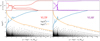 |
Fig. 4. Lamb and Brunt-Väisälä frequencies (lower panels) and the chemical profile (upper panels) for the same models shown in Fig. 3. In the lower panels, the black dots indicate the location of the nodes (zero displacement) of the radial eigenfunctions of g modes. |
3.1. Periods
In the upper panels of Fig. 5, we show the differences between the periods of the VLHF and VLTP models for Teff values of 30 000 K and 22 000 K. In the lower panels, we show those differences relative to the periods of the VLHF models for the same temperatures. All of the differences are between periods with the same radial order k. In the case of g modes, lower radial orders correspond to shorter periods. De Gerónimo et al. (2017) found that the differences in periods of a pulsating H-rich WD (DAV WD) model that has experienced three thermal pulses as opposed to one that has not experienced thermal pulses are less than 15 s for 0.548 M⊙ in the period range of DA WD stars, at Teff = 12 000 K. In contrast to this result, for our H-deficient WDs, we find that the differences of periods between no thermal pulses (VLHF) and two thermal pulses (VLTP) can be as high as 100 s for k = 23 – corresponding to a period of 1080 s for the VLHF – and they grow with higher values of k. This is probably due to the differences in the asymptotic period spacing of the models (see Sect. 3.2). Also, we find that the periods for the VLHF models are systematically higher than the periods of the VLTP models, except for k = 1. All of the differences are due to both the existence of the intershell region and the shift outward of the C-He transition region in the case of the VLTP models, in comparison with the VLHF case. The higher differences compared to the ones found for H-rich pulsating WDs by De Gerónimo et al. (2017) may be related to the fact that we are comparing a model that went through the AGB and the thermally-pulsing phase with one that avoided the AGB phase. In De Gerónimo et al. (2017), all of the models that they compare went through the AGB phase, even if they avoided the thermally-pulsing phase. Therefore, the chemical profiles that they compare show less-pronounced differences than the ones that we compare in this work. Also, the different results may be related to the difference in mass and temperature of our models with respect to the ones of De Gerónimo et al. (2017). Due to the mass-radius relation for WDs, more massive WDs are more dense stars and, therefore, the Brunt-Väisälä frequency is higher. This means that the period spectrum of more massive models moves to shorter values compared to less massive models. As a consequence, absolute differences in periods when comparing higher-mass models are expected to be lower than in lower-mass models. In addition, diffusion processes are still very active at the temperatures of pulsating DB stars, and the differences in the chemical profile are more pronounced than at lower temperatures (Teff ∼ 12 000 K) where DAV stars pulsate.
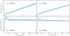 |
Fig. 5. Difference between periods (blue lines) and asymptotic period spacings (horizontal full gray lines) of the VLHF and the VLTP models with the same radial order k versus the periods of the VLHF models for Teff = 30 000 K and 22 000 K (upper panels), and the same differences but relative to the periods of the VLHF models (lower panels). |
Though the higher differences are found for longer periods – i.e., higher values of k – the higher relative differences are found for periods with radial orders up to k = 10; being the highest difference reached at k = 4 (about 12%, see Fig. 5, lower panel). The horizontal line in the plots is the relative difference between the asymptotic period spacings. The relative differences in periods vary around this value, specially for high values of k. This shows that the differences at long periods (P > 600 s) are mainly due to the differences in the asymptotic period spacings, and the differences at short periods (P < 600 s) are also due to the differences in the chemical profiles.
The important differences found in the periods of VLHF and VLTP models of the same mass and temperatures suggest that it might be possible to infer valuable information about the evolutionary history of low-mass DB WDs by means of asteroseismic period-to-period fits of DBV stars.
3.2. Period spacings
In Fig. 6 we show the period spacings, ΔP, which are the differences between consecutive periods from the same model. We compare the periods spacings for both evolutionary scenarios at Teff = 30 000 K and 22 000 K. We plotted, for comparison purposes, the asymptotic period spacings (ΔP when k → ∞). In all cases, the period-spacing distribution show mode-trapping substructures that change as diffusion acts. However, these trapping substructures are somewhat different for the two scenarios, in particular the trapping amplitudes. At both values of Teff, the trapping amplitude of the VLHF model is higher for periods between ≃100–400 s. In fact, as previously discussed in Sect. 3.1, this range of periods is the most affected by the differences in the chemical profiles. Therefore, measuring period spacings between periods in the range of 100–400 s can also help us to determine the evolutionary history of low-mass DB WDs.
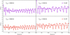 |
Fig. 6. Period spacings (ΔP) versus periods for the VLTP case (red lines, lower panels) and the VLHF case (violet lines, upper panels), for Teff = 30 000 K (right panels) and Teff = 22 000 K (left panels). Horizontal lines show the corresponding asymptotic period spacings. |
Above q ∼ 0.5, the Brunt-Väisälä frequency of the VLTP model is somewhat higher than in the VLHF model. This is due to the existence of the intershell region and the location of the C-He transition region in the VLTP model. The differences in N in both models make the asymptotic period spacings slightly differ for about 2–3 s for all temperatures. Therefore, even if we were able to measure sufficient periods in a pulsating low-mass DB WD in order to determine a mean period spacing, that would likely be useless in distinguishing between the two scenarios.
3.3. Period drifts
Another observable quantity from pulsations in WDs is the rate of change of periods (period drifts, Ṗ). Due to the difficulty in finding stable periods in DBVs, a reliable measurement of the period drift of a DB WD is lacking. However, Redaelli et al. (2011) derived an estimate for the period drift of the DBV star PG 1351+489. We calculated the period drifts of the models to see if future determinations of Ṗ in DBVs could help us to determine their evolutionary history. In Fig. 7 we plotted the period drifts relative to periods of the same models shown in Figs. 5 and 6. We can see that for Teff = 30 000 K, the mean value of the period drifts for the VLHF model is larger than for the VLTP model, but this is not true for all the periods. Therefore, it is not likely that determining one period drift would help us to distinguish between the models. In the case of Teff = 22 000 K, there are almost no differences in the values of Ṗ. The period drift of both DAVs and DBVs are related to their cooling rates (Althaus et al. 2010). At Teff = 30 000 K, the VLHF model evolves faster than the VLTP model, but this is not the case shortly after, therefore, we do not expect significant differences in Ṗ for temperatures below Teff = 30 000 K. As the period drifts for the models of VLHF and VLTP do not exhibit significant differences, measuring a period drift of low-mass DB WDs would not help us in distinguishing between VLTP and VLHF models – unless we were able to measure the period drift for several periods of a star with Teff ∼ 30 000 K.
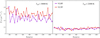 |
Fig. 7. Period drifts (Ṗ) relative to periods (P) versus periods for the VLTP case (red lines) and the VLHF case (violet lines), for Teff = 30 000 K (right panel) and Teff = 22 000 K (left panel). |
4. Discussion and conclusions
In this work, we compare the pulsation properties of low-mass DB WD models that came from a very-late thermal pulse after the AGB phase with models that experienced a late helium flash onset in an almost stripped core of a red giant star. We find that these two evolutionary channels for the formation of low-mass (∼0.46 M⊙) H-deficient WDs lead to very different chemical profiles at the WD stage. As a consequence, the Brunt-Väisälä frequencies of the models at the instability strip of DBVs exhibit different features that translate into different properties of the g-mode pulsation spectrum. In particular, the periods in the range of 100–400 s are more sensitive to the distinct features of the chemical profiles, showing different mode-trapping substructures. This implies that both period-to-period fits of DB WDs and the measurement of the period spacings in the mentioned range of periods can help in determining the evolutionary history of low-mass DB WDs. In contrast, mean period spacings and period drift measurements likely do not help in distinguishing between the two evolutionary scenarios. These last two quantities are more complicated to determine for DBVs because of the low number of periods usually observed in WDs and the difficulty in finding stable periods in pulsating DB WDs, in particular. Therefore, we conclude that both a comprehensive analysis of the observed period spacings in pulsating low-mass DB WDs, especially in the range of periods below 500 s, and detailed asteroseismic period-to-period fits of these stars could help to shed light on their evolutionary history.
Acknowledgments
We cordially thank the anonymous referee for a constructive report that improved the presentation of this work. We thank Marcelo Miller Bertolami for useful discussions. Part of this work was supported by AGENCIA through the Programa de Modernización Tecnológica BID 1728/OC-AR, by the PIP 112-200801-00940 grant from CONICET and by the G149 grant from the National University of La Plata. This research has made use of NASA’s Astrophysics Data System.
References
- Althaus, L. G., Serenelli, A. M., Panei, J. A., et al. 2005, A&A, 435, 631 [NASA ADS] [CrossRef] [EDP Sciences] [Google Scholar]
- Althaus, L. G., Córsico, A. H., Isern, J., & García-Berro, E. 2010, A&ARv, 18, 471 [NASA ADS] [CrossRef] [Google Scholar]
- Althaus, L. G., De Gerónimo, F., Córsico, A., Torres, S., & García-Berro, E. 2017, A&A, 597, A67 [NASA ADS] [CrossRef] [EDP Sciences] [Google Scholar]
- Battich, T., Miller Bertolami, M. M., Córsico, A. H., & Althaus, L. G. 2018, A&A, 614, A136 [NASA ADS] [CrossRef] [EDP Sciences] [Google Scholar]
- Beauchamp, A., Wesemael, F., Bergeron, P., Liebert, J., & Saffer, R. A. 1996, in Hydrogen Deficient Stars, eds. C. S. Jeffery, & U. Heber, ASP Conf. Ser., 96, 295 [NASA ADS] [Google Scholar]
- Bergeron, P., Leggett, S. K., & Ruiz, M. T. 2001, ApJS, 133, 413 [NASA ADS] [CrossRef] [Google Scholar]
- Bergeron, P., Wesemael, F., Dufour, P., et al. 2011, ApJ, 737, 28 [NASA ADS] [CrossRef] [EDP Sciences] [Google Scholar]
- Bergeron, P., Dufour, P., Fontaine, G., et al. 2019, ApJ, 876, 67 [NASA ADS] [CrossRef] [Google Scholar]
- Brown, T. M., Sweigart, A. V., Lanz, T., Landsman, W. B., & Hubeny, I. 2001, ApJ, 562, 368 [NASA ADS] [CrossRef] [Google Scholar]
- Cassisi, S., Schlattl, H., Salaris, M., & Weiss, A. 2003, ApJ, 582, L43 [NASA ADS] [CrossRef] [Google Scholar]
- Castellani, M., & Castellani, V. 1993, ApJ, 407, 649 [NASA ADS] [CrossRef] [Google Scholar]
- Córsico, A. H., Althaus, L. G., & Miller Bertolami, M. M. 2006, A&A, 458, 259 [NASA ADS] [CrossRef] [EDP Sciences] [Google Scholar]
- Córsico, A. H., Althaus, L. G., Miller Bertolami, M. M., & Kepler, S. O. 2019, A&ARv, 27, 7 [NASA ADS] [CrossRef] [Google Scholar]
- De Gerónimo, F. C., Althaus, L. G., Córsico, A. H., Romero, A. D., & Kepler, S. O. 2017, A&A, 599, A21 [NASA ADS] [CrossRef] [EDP Sciences] [Google Scholar]
- Fontaine, G., & Brassard, P. 2008, PASP, 120, 1043 [NASA ADS] [CrossRef] [Google Scholar]
- Genest-Beaulieu, C., & Bergeron, P. 2019a, ApJ, 871, 169 [NASA ADS] [CrossRef] [Google Scholar]
- Genest-Beaulieu, C., & Bergeron, P. 2019b, ApJ, 882, 106 [NASA ADS] [CrossRef] [Google Scholar]
- Gentile Fusillo, N. P., Tremblay, P.-E., Gänsicke, B. T., et al. 2019, MNRAS, 482, 4570 [NASA ADS] [CrossRef] [Google Scholar]
- Han, Z., Podsiadlowski, P., Maxted, P. F. L., & Marsh, T. R. 2003, MNRAS, 341, 669 [NASA ADS] [CrossRef] [Google Scholar]
- Iben, I., Jr 1976, ApJ, 208, 165 [NASA ADS] [CrossRef] [Google Scholar]
- Iben, I., Jr, Kaler, J. B., Truran, J. W., & Renzini, A. 1983, ApJ, 264, 605 [NASA ADS] [CrossRef] [Google Scholar]
- Jeffery, C. S., Karakas, A. I., & Saio, H. 2011, MNRAS, 414, 3599 [NASA ADS] [CrossRef] [Google Scholar]
- Kepler, S. O., Pelisoli, I., Koester, D., et al. 2019, MNRAS, 486, 2169 [NASA ADS] [Google Scholar]
- Koester, D., & Kepler, S. O. 2015, A&A, 583, A86 [NASA ADS] [CrossRef] [EDP Sciences] [Google Scholar]
- Lanz, T., Brown, T. M., Sweigart, A. V., Hubeny, I., & Landsman, W. B. 2004, ApJ, 602, 342 [NASA ADS] [CrossRef] [Google Scholar]
- Lauer, A., Chatzopoulos, E., Clayton, G. C., Frank, J., & Marcello, D. C. 2019, MNRAS, 488, 438 [NASA ADS] [CrossRef] [Google Scholar]
- Longland, R., Lorén-Aguilar, P., José, J., et al. 2011, ApJ, 737, L34 [NASA ADS] [CrossRef] [Google Scholar]
- Miller Bertolami, M. M. 2016, A&A, 588, A25 [NASA ADS] [CrossRef] [EDP Sciences] [Google Scholar]
- Miller Bertolami, M. M., Althaus, L. G., Serenelli, A. M., & Panei, J. A. 2006, A&A, 449, 313 [NASA ADS] [CrossRef] [EDP Sciences] [Google Scholar]
- Miller Bertolami, M. M., Althaus, L. G., Unglaub, K., & Weiss, A. 2008, A&A, 491, 253 [NASA ADS] [CrossRef] [EDP Sciences] [Google Scholar]
- Oke, J. B., Weidemann, V., & Koester, D. 1984, ApJ, 281, 276 [NASA ADS] [CrossRef] [Google Scholar]
- Ourique, G., Romero, A. D., Kepler, S. O., Koester, D., & Amaral, L. A. 2019, MNRAS, 482, 649 [NASA ADS] [CrossRef] [Google Scholar]
- Paczynski, B. 1976, in Structure and Evolution of Close Binary Systems, eds. P. Eggleton, S. Mitton, & J. Whelan, IAU Symp., 73, 75 [NASA ADS] [CrossRef] [EDP Sciences] [Google Scholar]
- Redaelli, M., Kepler, S. O., Costa, J. E. S., et al. 2011, MNRAS, 415, 1220 [NASA ADS] [CrossRef] [Google Scholar]
- Reindl, N., Rauch, T., Werner, K., et al. 2014a, A&A, 572, A117 [NASA ADS] [CrossRef] [EDP Sciences] [Google Scholar]
- Reindl, N., Rauch, T., Werner, K., Kruk, J. W., & Todt, H. 2014b, A&A, 566, A116 [NASA ADS] [CrossRef] [EDP Sciences] [Google Scholar]
- Renzini, A. 1979, in Stars and Star Systems, ed. B. E. Westerlund, Astrophys. Space Sci. Lib., 75, 155 [NASA ADS] [CrossRef] [Google Scholar]
- Renzini, A. 1981, in IAU Colloq. 59: Effects of Mass Loss on Stellar Evolution, eds. C. Chiosi, & R. Stalio, Astrophys. Space Sci. Lib., 89, 319 [NASA ADS] [CrossRef] [Google Scholar]
- Saio, H., & Jeffery, C. S. 2002, MNRAS, 333, 121 [NASA ADS] [CrossRef] [Google Scholar]
- Schoenberner, D. 1979, A&A, 79, 108 [NASA ADS] [Google Scholar]
- Schwab, J. 2018, MNRAS, 476, 5303 [NASA ADS] [CrossRef] [Google Scholar]
- Shipman, H. L. 1979, ApJ, 228, 240 [NASA ADS] [CrossRef] [Google Scholar]
- Sweigart, A. V. 1997, ApJ, 474, L23 [NASA ADS] [CrossRef] [Google Scholar]
- Tailo, M., D’Antona, F., Vesperini, E., et al. 2015, Nature, 523, 318 [NASA ADS] [CrossRef] [Google Scholar]
- Tremblay, P. E., Cukanovaite, E., Gentile Fusillo, N. P., Cunningham, T., & Hollands, M. A. 2019, MNRAS, 482, 5222 [NASA ADS] [CrossRef] [EDP Sciences] [Google Scholar]
- Villanova, S., Geisler, D., Piotto, G., & Gratton, R. G. 2012, ApJ, 748, 62 [NASA ADS] [CrossRef] [Google Scholar]
- Voss, B., Koester, D., Napiwotzki, R., Christlieb, N., & Reimers, D. 2007, A&A, 470, 1079 [NASA ADS] [CrossRef] [EDP Sciences] [Google Scholar]
- Webbink, R. F. 1984, ApJ, 277, 355 [NASA ADS] [CrossRef] [Google Scholar]
- Winget, D. E., & Kepler, S. O. 2008, ARA&A, 46, 157 [NASA ADS] [CrossRef] [EDP Sciences] [Google Scholar]
- Zhang, X., & Jeffery, C. S. 2012, MNRAS, 419, 452 [NASA ADS] [CrossRef] [Google Scholar]
All Figures
|
Fig. 1. Hertzsprung-Russell diagram for the VLTP scenario (left) and the VLHF scenario (right) computed from the main sequence to the WD stage. In both panels, the star symbol marks the model where the maximum CNO-luminosity of the H flash occurs. In the right panel, we show the location of the models of Fig. 2 (a, b, c, and d), and the model of the right panel of Fig. 3 (e). |
| In the text | |
|
Fig. 2. Oxygen (O), carbon (C), and helium (He) profiles of the models highlighted in Fig. 1 with letters a, b, c, and d. |
| In the text | |
|
Fig. 3. Oxygen (O), carbon (C), and helium (He) profiles of WD models coming from a VLTP (left) and a VLHF (right) at Teff = 30 000 K. |
| In the text | |
|
Fig. 4. Lamb and Brunt-Väisälä frequencies (lower panels) and the chemical profile (upper panels) for the same models shown in Fig. 3. In the lower panels, the black dots indicate the location of the nodes (zero displacement) of the radial eigenfunctions of g modes. |
| In the text | |
|
Fig. 5. Difference between periods (blue lines) and asymptotic period spacings (horizontal full gray lines) of the VLHF and the VLTP models with the same radial order k versus the periods of the VLHF models for Teff = 30 000 K and 22 000 K (upper panels), and the same differences but relative to the periods of the VLHF models (lower panels). |
| In the text | |
|
Fig. 6. Period spacings (ΔP) versus periods for the VLTP case (red lines, lower panels) and the VLHF case (violet lines, upper panels), for Teff = 30 000 K (right panels) and Teff = 22 000 K (left panels). Horizontal lines show the corresponding asymptotic period spacings. |
| In the text | |
|
Fig. 7. Period drifts (Ṗ) relative to periods (P) versus periods for the VLTP case (red lines) and the VLHF case (violet lines), for Teff = 30 000 K (right panel) and Teff = 22 000 K (left panel). |
| In the text | |
Current usage metrics show cumulative count of Article Views (full-text article views including HTML views, PDF and ePub downloads, according to the available data) and Abstracts Views on Vision4Press platform.
Data correspond to usage on the plateform after 2015. The current usage metrics is available 48-96 hours after online publication and is updated daily on week days.
Initial download of the metrics may take a while.