| Issue |
A&A
Volume 638, June 2020
|
|
|---|---|---|
| Article Number | A27 | |
| Number of page(s) | 14 | |
| Section | Catalogs and data | |
| DOI | https://doi.org/10.1051/0004-6361/202037726 | |
| Published online | 04 June 2020 | |
A redshift database towards the Shapley supercluster region⋆,⋆⋆
1
Instituto de Astrofísica, Facultad de Física, Pontificia Universidad Católica de Chile, Casilla 306, Santiago 22, Chile
2
GEPI, Observatoire de Paris, 92195 Meudon Principal CEDEX, France
e-mail: This email address is being protected from spambots. You need JavaScript enabled to view it.
3
Gemini Observatory, NSF’s National Optical-Infrared Astronomy Research Laboratory, Casilla 603, La Serena 1700000, Chile
Received:
13
February
2020
Accepted:
2
April
2020
Abstract
We present a database and catalogue of radial velocities of galaxies towards the region of the Shapley Supercluster (SSC) based on 18 129 measured velocities for 10 702 galaxies in the approximately 300 square degree area between 12h43m00s < RA < 14h17m00s and −23° 30′00″ > Dec > − 38° 30′00″. The database contains velocity measurements that have been reported in the literature up until 2015. It also includes 5084 velocities, corresponding to 4617 galaxies, observed by us at Las Campanas Observatory and Cerro Tololo Inter-American Observatory, which had not been reported individually until now. Of the latter, 2585 correspond to galaxies with no other previously published velocity measurement before 2015. Every galaxy in the velocity database has been identified with a galaxy extracted from the SuperCOSMOS photometric catalogues. We also provide a combined average velocity catalogue for all 10 702 galaxies with measured velocities, adopting the SuperCOSMOS positions as a homogeneous base. A general magnitude cut-off at R2 = 18.0 mag was adopted (with exceptions only for some of the new reported velocities). In general terms, we confirm the overall structure of the SSC as reported in earlier papers. However, the more extensive velocity data show finer structures, which is to be discussed in a future publication.
Key words: galaxies: distances and redshifts
The complete versions of Tables 2 and 4 are only available at the CDS via anonymous ftp to cdsarc.u-strasbg.fr (130.79.128.5) or via http://cdsarc.u-strasbg.fr/viz-bin/cat/J/A+A/638/A27
Based on observations made at Las Campanas Observatory (Chile) and Cerro-Tololo Interamerican Observatory (Chile).
© H. Quintana et al. 2020
 Open Access article, published by EDP Sciences, under the terms of the Creative Commons Attribution License (https://creativecommons.org/licenses/by/4.0), which permits unrestricted use, distribution, and reproduction in any medium, provided the original work is properly cited.
1. Introduction
Superclusters of galaxies are the largest structures that can be identified in large redshift surveys of galaxies or in catalogues of clusters of galaxies, of sizes ∼100 Mpc. With densities a few times larger than the average density of the Universe, they are already in the non-linear regime, but still far from being virialized (contrary to clusters of galaxies). Thus, their complex spatial and velocity structure still largely reflect their initial conditions and their limits are ill-defined and dependent on arbitrary criteria such as density thresholds or linking lengths.
Dünner et al. (2006) proposed a physical definition of superclusters as the largest structures that remain bound in spite of the accelerated expansion of the Universe and eventually collapse to form stable, virialized, spherical clusters that separate from each other at exponentially increasing velocities in the future (e.g. Araya-Melo et al. 2009). In a spherical model, the outermost shell of a bound structure of mass M approaches an asymptotic radius (3GM/Λ)1/3 (where G is Newton’s gravitational constant and Λ is Einstein’s cosmological constant), corresponding to an average enclosed matter density twice that associated with the cosmological constant, ρΛ ≡ Λ/(8πG). In the present Universe (with density parameters Ωm = 0.3 and ΩΛ = 0.7), the enclosed matter density is still 1.69 times higher than this asymptotic value, corresponding to 2.36 times the current critical density or 7.87 times the current average matter density of the Universe (Chiueh & He 2002; Dünner et al. 2006). The density threshold set by this criterion is rather high compared to those usually chosen to define superclusters, implying that most of the mass of observationally defined superclusters is actually not bound, and the physical definition yields smaller superclusters, as found, for example, by Chon et al. (2013). In order to distinguish these two definitions, Chon et al. (2015) proposed calling the latter “superstes clusters” (“survivor clusters”), as they are expected to survive the accelerated expansion.
In the nearby Universe, at redshifts z < 0.1, several superclusters have been identified, including our own. Tully et al. (2014) have proposed an extension of our own supercluster, where the Local Group and Milky Way reside, from an analysis of the results of the extensive Cosmic Flows surveys undertaken by their group, which includes new galaxies found in the traditional zone of avoidance. These numerous galaxies form a connection between the Virgo supercluster and other nearby structures, including 13 Abell clusters, forming a larger entity named the Laniakea supercluster, with a diameter of 160 Mpc (equivalently, 12 000 km s−1 in velocity) and a total mass of 1017 M⊙. However, the density enhancement and dynamical state of the Laniakea supercluster lead to the prediction (Chon et al. 2015) that the whole structure is unbound and will disperse due to the effect of dark energy in the long-term future (with some substructures or clusters remaining bound).
The more distant “Shapley Concentration” or “Shapley Supercluster” (SSC) at z ≈ 0.05 was long ago recognized as one of the largest structures in the nearby Universe (Shapley 1930). Melnick & Quintana (1981) were the first to identify the central cluster, later named A3558 (Abell et al. 1989), as a bright X-ray cluster. Subsequently, Melnick & Moles (1987) studied the several major clusters and main groups in the central regions, using data later published by Quintana et al. (1995), where the general supercluster structure was further defined. Its unique position within the z < 0.1 Universe was pointed out by Raychaudhury (1989) and Scaramella et al. (1989).
Catalogues of superclusters (Einasto et al. 2001, 2003a,b) find the SSC to be the largest and richest supercluster at z < 0.1, with its 28 suggested cluster members (although Chon et al. 2013 find it to split up into several “superstes clusters”). As such, given its dominant position, it can play an important role in constraining models of structure formation (Sheth & Diaferio 2011). It has also been invoked as being responsible for the motion of the Local Group with respect to the cosmic microwave background (e.g. Melnick & Moles 1987; Kocevski et al. 2004; Hoffman et al. 2017). In addition, it is an interesting laboratory to understand the interactions between clusters of galaxies, as well as the evolution of galaxies in high-density regions, but before falling into clusters (Merluzzi et al. 2013, 2016). For such applications, it is necessary to accurately characterise the structure and dynamics of the supercluster, in order to measure its total mass and density distribution and assess the evolutionary state of its different regions. This requires large redshift surveys, which in fact have been carried out over the years (Quintana et al. 2000; Proust et al. 2006; Haines et al. 2018, and references therein).
Over the last few years, the number of velocity measurements in this direction has been rapidly increasing, mainly thanks to multi-object spectroscopic surveys such as FLASH (Kaldare et al. 2003), 6dF (Jones et al. 2009), and many observations by our group. Recently, Haines et al. (2018) presented a deep, highly complete redshift survey of the SSC’s core region (21 square degrees or [17 Mpc]2) and a detailed analysis of the structure in the core region, following early work on the core region by Bardelli et al. (1998a).
In this paper, we present a compilation of velocities in a wide area (20° ×15°), including our previously unreported data. The latter were obtained mainly from a survey carried out over several years with the fiber and multislit spectrographs at the 100″ du Pont telescope at Las Campanas Observatory (LCO), as well as the Hydra spectrograph at the Blanco 4.0 m telescope at Cerro-Tololo Interamerican Observatory (CTIO). Here, we present all the data resulting from these observations, which represent a set of 5084 new velocities among which 2585 are newly observed galaxies. Combining them with already published redshift sets from several surveys and papers, compiled until 2015, we built up the most extensive velocity database for the SSC area, containing 18 129 velocity measurements for 10 702 galaxies.
The observing runs and instrumentation used in the spectroscopic observations are described in Sect. 2. In Sect. 3, we present the extraction and build-up of a photometric galaxy catalogue from the SuperCOSMOS Sky Surveys (hereafter SSS)1 for the approximately 300 square degree area of the sky. The extended velocity database is described in Sect. 4, while Sect. 5 describes the average velocity and photometry catalogue, obtained from cross-combining the velocities from the database with the photometry and astrometry from the galaxy catalogue derived from the SSS. This section includes comparisons between the galaxy velocities in common among different data sets, as well as the velocity zero-point shifts required to equalise the combined average catalogue. In Sect. 6, we discuss the completeness of this average velocity catalogue and analyse the galaxy number density over the whole area. Finally, Sect. 7 describes the observed galaxy density, velocity distribution, and general structure of the supercluster.
2. Observations and instrumentation
The selected SuperCOSMOS region extends in Right Ascension (RA) from 12:44:50.557 to 14:17:43.609 and in Declination (Dec) from −38:30:03.41 to −23:27:30.24, containing 60710 objects identified by us as galaxies. The galaxy positions, photometric magnitudes (R1, R2, Bj, and I), and morphological properties were inherited from the SuperCOSMOS values.
The spectroscopic observations were carried out using initially the fiber spectrograph and then the Wide-Field CCD (WFCCD), both mounted on the 2.5 m du Pont telescope at LCO, Chile2, and the Hydra fiber spectrograph on the 4.0 m Blanco telescope at CTIO, Chile3.
The multi-fiber system first used at LCO consists of a plug plate at the focal plane, with 128 fibers running to a spectrograph coupled to the 2D-Frutti detector, covering a field of view of 1.5 × 1.5 degrees on the sky. Instrumental details and observing procedures were the same as on earlier reported observations described in Shectman (1989), Quintana et al. (2000), and Proust et al. (2006).
The WFCCD is a multi-slit drilled bronze mask with useful 22 arcmin × 22 arcmin field of view, taking two fields per cluster to cover central regions. Blue grism 400 lines mm−1 was used for spectra exposure, with a 2k × 2k CCD, binned 1 × 1 with gain 1. We took three or four 900s exposures per field, and He-Ar comparison lamps were taken before and immediately after each set of exposures.
Hydra is a multi-object spectrograph with 138 fibers of 2 arcsec diameter on the sky operating in a 40 arcmin diameter field of view. It uses a 400 mm camera and SITe 4k × 2k detector, binning 1 × 2 with gain 2, noise 3e− with filter GG385. The KPGL2 grating resolution was 0.7 Å pix−1 with a spectral range 3600–7400 Å mm−1 and tilt 5.74°. We made three exposures of 480 s, 720 s, or 1200 s depending on the average brightness of the galaxies in the field.
Table 1 gives a schedule of the observing sessions and a code for the corresponding observation sets used in the following Database. In Fig. 1 we plot the fields covered by the spectroscopic observations, as explained in its caption. Three missing fields shown by the gaps between Dec −33° and Dec −36°, were partly due to poor weather conditions in 1998 and 1999 runs. These could not be repeated because the instrument was retired.
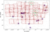 |
Fig. 1. Spectroscopic survey fields reported in this paper. Large squares are LCO fiber spectrograph observations. Circles are Hydra fields observed at CTIO, and small blue squares are WFCCD fields observed at LCO. The area of this plot is smaller than the total catalogue area, chosen to zoom in on the surveyed fields. The gray dots represent the positions of all galaxies in the velocity catalogue. Red dots are the positions of those galaxies whose velocities were measured by our group and reported in this paper. |
Observing sessions and instrumentation used.
From the above observing runs, we obtained a set of 5084 new velocities for 4617 galaxies (some of them were observed two or more times) in the general direction of the SSC.
3. Photometric and astrometric catalogue
One underlying problem with data collected from many sources over a period of many years comes from the (usually small) differences in the positions assigned to the galaxies in different surveys. Assuming there are no ambiguities in identification, the different positions quoted in the literature (particularly in older data) make it hard in some cases to cross-identify the velocities in an automatic, homogeneous way. However, there are also some cases of ambiguities in identification, some due to misprints in listed positions, juxtaposition of (brighter) large galaxies to faint nearby ones, or due to crowding and superposition of galaxies near cluster or groups centers. Older data come from many sources, with varying positional errors. If we include HIPASS observations, as we did, position errors can reach up to 6′ (Doyle et al. 2005). A valuable tool became available in the South with the access to the SuperCOSMOS Sky Surveys (SSS) facility with homogeneous astrometry and photographic photometry. SSS provides digitized scans of the B(J), R (R1 and R2), and I color band Sky Surveys plates, with a pixel size of 0.7 arcsec. The SSS is available from the Web, including downloads of images and extraction catalogue of objects according to different parameter choices.
The extraction of object catalogues from the SSS was done with the parameter set left at their suggested default values, except image quality, as discussed in what follows. Two parameters of particular relevance were the Classification flag (1 = galaxy, 2 = star, 3 = unclassifiable, 4 = noise), and the Quality flag, specifying an object’s image quality (see SSS). Two files were produced, one for Class 1 objects, in principle classified as galaxies, and one for Class 2 objects, in principle stars. Below we discuss these classifications in more detail. Class 3 or 4 objects were extremely few; they were analysed and eventually considered not relevant for the study.
Images and object catalogues were extracted in an area centered near the position of the central cluster A3558: RA(2000) 13:30:00, Dec (2000) −31:30:00. We chose the output with the suggested most useful subset of master IAM (Image Analysis Mode) data as suitable for our purpose. Images were extracted with 30′ × 30′ size. The object catalogues produce positions, proper motions (disregarded), magnitudes in all four bands, image ellipticity fits, position angle, ellipse area, image quality, and class. The ESO SkyCat software package4 permits to display the survey images overlapped by the object catalogues, each object represented by an ellipse with its center coordinates, area, ellipticity, and position angle parameters. Different colors or symbols also allow simultaneous overlays of several catalogues. Due to the not uncommon presence of blended galaxy images in clusters, we kept both the parent object defined by the common low isophotal contour and the daughter objects, represented by ellipses around the individual galaxies, at higher isophote contours. In the visual analysis, we chose the most representative isophote for each galaxy image, deleting the rest. We used the standard pairing distance of 3″. From many trials by visual inspection, we found that the suggested default quality flag extraction value 128 missed too many real galaxy images in the neighbourhood of bright stars, because of contamination by reflections and spikes. Therefore, the quality parameter was chosen as 4096 to extract basically all the galaxy images, from an upper magnitude limit of R2 = 10 down to a lower limit of R2 = 18.0 mag, as the red R magnitude is more representative of cluster galaxies. However, we found the B images were better to distinguish by eye between galaxies, stars, and spurious objects thanks to the better image quality and contrast of galaxy disks and halos in this band.
The catalogue area extracted extends over 300 square degrees (exactly 301.3), between 12h43m00s < RA(2000) < 14h17m00s and −23° 31′00″ > Dec(2000) > − 38° 30′00″. In this way we covered nearly the complete area of possible SSC candidate clusters (including the WFCCD observations). Several extracted partial catalogues were merged, carefully avoiding duplication of objects on the overlapping border areas. In total, we extracted 1300 images of 30′ × 30′ in size (in a 42 × 31 grid, with a 1 arcmin overlap to avoid missing sky areas or objects near the edges), and all 1300 fields were searched by eye to clean the catalogues by removing spurious objects and repeated isophotal contours.
The 30′ × 30′ survey image fields were first looked at on the screen in sections of 10′ × 10′, when the first clean-up of the galaxy (Class 1) object catalogue performed, eliminating obvious reflections and star spikes, plate defects, and other noise. For some rather bright galaxies, several elliptical isophotal contours were given, of which we chose the lower, wider area ellipse representative object, that had a center coincident with the galaxy optical center. Examples of not so faint double stars, identified by a common ellipse as Class 1, were deleted. In case of doubts, usually due to faint double star images identified as a single object, we looked at higher magnification. The observed inhomogeneous plate image quality, as well as increasing star numbers and image confusion at lower Galactic latitudes (towards the south), both combined to make the selection easier in the cleaner Northern sections of the area and increasingly harder in the Southern region. The number of spurious objects extracted from the catalogue classified as Class 1 was large, in some survey plates several times larger than the actual galaxy number. Needless to say, this was the effect of using the value 4096 as image quality, but also of the increasing number of stars and worse seeing at lower Galactic latitudes. Thus, at lower Galactic latitudes, where the star density more than doubles that present at higher latitudes, worse seeing in an original plate would produce more objects spuriously classified as galaxies due to image diffusion and blended images of close faint optical star pairs. These effects introduce an unavoidable systematic effect in the catalogue, increasing the uncertainty of its completeness near the limiting magnitude in those fields. In summary, among the objects extracted as Class 1 (in principle classified as galaxies) with our chosen parameters, in each 30′ × 30′ survey image field between 40% and 85% of objects (depending on its declination and presence of bright stars) were found not to be galaxies, but different kinds of other objects, as described above. The actual numbers vary widely if the field fell on a cluster or a fairly empty region.
There are additional factors that increase photometric and positional uncertainties of some catalogue objects. These effects are caused by galaxy-star or galaxy-galaxy superpositions, not properly deblended by the catalogue software, and depend on the density of galaxies and stars, which vary with field positions (e.g. if they fall on galaxy clusters) and with Galactic latitude. Therefore, across the whole supercluster area surveyed this effect is quite variable. Of order 15% of objects catalogued as galaxies have photometric or positional parameters distorted (in most cases only slightly) by superposition of images of two galaxies or a galaxy and a star.
The procedures applied were as follows:
(a) Galaxy-star super or juxtapositions. When the dominant part of the image was a star (producing most of the magnitude) over a very faint galaxy these catalogue objects were eliminated. When the star was a perturbation of similar or smaller magnitude to the galaxy image, these objects were retained in the galaxy catalogue (with the resulting parameter values). Naturally, the photometry values would be in error, but a significant galaxy could be retained. However, the fitted ellipse was also distorted and its center position altered. No sharp limit between these cases could be used, as it depended on relative magnitudes and center distances, galaxy shape, and seeing. In a few cases, when the center of the galaxy isophote was off by several seconds and there was a velocity measured, we corrected the center position to the center of the galaxy to aid the correct identification.
(b) Galaxy-galaxy superpositions. When the de-blending procedure worked, we kept both separate ellipse objects as galaxies. However, in many cases this did not happen. When one galaxy was much fainter than the companion, we kept the catalogue object as given. If we did not have velocities for either component, we did similarly. For galaxies brighter than around R2 = 17.0, if two galaxy images in contact were represented by one entry and we had some component velocity, we extracted a catalogue over a small area trying different extraction parameters, to check if merged or parent and daughter images were available that solved the problem. However, when this procedure did not work, we added another entry by hand, adjusting both positional and angle parameters to represent the two galaxies as separate objects (duplicating the photometry). These procedures were important in the centers of clusters, when bright dumbbell galaxies or several superimposed galaxies were present (most with velocities measured). In this way, we tried to keep the galaxy identification correct and complete (to correlate with the velocities).
A rare, but non-negligible situation arose occasionally, first discovered when the position assigned to a velocity measurement fell on top of a relatively bright elliptical galaxy image not appearing in the Class 1 objects. We looked at the Class 2 catalogue and found a corresponding object. Because we found several other cases, with or without velocities, we looked on the screen at the whole catalogue of Class 2 objects overlapped on the survey images. Occasionally, we found obvious (fairly bright) galaxies wrongly classified as stars, of order 2–3 per square degree. These were fairly bright E0 ellipticals, with clear diffuse edges. We transferred these entries to the galaxy catalogue but kept their Class 2 for easy later reference. As a further step in the verification of the galaxy identifications we simultaneously plotted the NED database5 with different symbols over the survey images. This was of particular help near the cut-off photometric limit R2 = 18.0 mag.
In total, we extracted more than 1 184 000 objects of all classes. The number of Class 2 (star) entries was roughly one million. The number of original Class 1 (galaxy) objects was close to 173 000. All of them were checked individually by eye6, as a majority were spurious or problematic classifications (as a result of using the quality image parameter 4096, as discussed). The number of galaxy objects kept was slightly more than 60 400. Thus, the number of real galaxies was around 30% of the Class 1 entries. To these entries, we added a few hundred additional galaxy entries. A few of these were generated “by hand” in the case of double or superimposed galaxies, as explained, or star images that turned out to be galaxies and moved to this catalogue. A few additional objects were galaxies fainter than R2 = 18.0 that had velocities measured by us (with a value within or close to the SSC velocity range). For the statistical analysis in Sect. 6, these faint galaxies were ignored by using the magnitude cut-off at R2 = 18.0 mag.
A further point needs to be discussed. The SSS software was designed to identify fairly faint galaxies. When galaxies are extended over several arcmin (i.e. galaxies with velocities less than ∼3000 km s−1, not members of the SSC), and particularly of low surface brightness, with several bright spots, the software produces isophotes centered at those bright spots, with no isophote describing the whole galaxy, neither well centered. Since these galaxies have photometry in the literature, we chose the partial isophote that appeared most precisely centered on the galaxy nucleus, to help the identification algorithm. For these extended area galaxies, the SSS optical parameters are not a good description of the image (see discussion in the HIPASS optical identification catalogue, Doyle et al. 2005).
The total number of galaxy entries in the derived SuperCOSMOS-based catalogue is 63 471 (with 294 fainter than R2 = 18.0 mag with new velocities). Hereafter, we call this the “Shapley area SSS galaxy catalogue”, or SASSSG catalogue, for short. A large majority of its galaxy entries have visually correct parameters (centers, magnitudes, ellipticities, and position angles).
4. Velocity database
By combining our new velocity measurements with existing ones from the literature, we produced a large velocity database containing 19 708 velocity measurements corresponding to 11 910 galaxies, over an area slighly bigger than the one finally chosen as defined earlier, and covering most of the SSC. When limited to the 300 square degrees, we obtained the quoted 18 129 velocities and 10 702 galaxies finally retained in the database.
Our search through the literature is not intended to be complete, particularly for velocities < 6000 km s−1. We added source references as we found them for one or another reason. We realize that several literature papers include previous data along with their own measurements, and thus the same velocity data point could inadvertently be considered several times, coming from different sources. A difficulty comes from the fact that in the literature the individual source of a velocity measurement is not always given. When the duplication is clear (because it coincides with an older value already included in the database), we eliminated the entry, keeping the original measurement. A comment was added in these entries. Moreover, there are references to databases dynamically varying in time, such as ZCAT7 or NED8. The FLASH survey uses these references as only source or to average values with their own measurements. If there has been an update of those databases, the sources of the old values may be lost or are hard to find. Moreover, when an author quotes a velocity that is an average of a new measurement with an older NED or ZCAT value, it is hard to know each of those values, specially if NED or ZCAT later updated their values exactly to the average given by the same reference rather than keeping the old value. Here we give individual velocity values with references for each of them, trying as much as possible to quote the original measurement only. However, when a literature average is given, we listed it as well, since it can contain new partial information from velocities unavailable today, for the reasons just given (and we warn about this in the comments). Generally we have also tried to give in the database the original numbers for the several parameters of the literature entry, as far as given by the authors.
We used the reported coordinates of each velocity measurement to compare with the SASSSG catalogue, grouping together multiple measurements of the same object, while identifying its visual counterpart. This was an iterative process done by finding the closest SASSSG galaxy counterpart to each entry in our preliminary database, up to a maximum allowable distance of 20″, and comparing cross-match velocities for consistency. The SSS images where used for visual inspection in the case of conflicts encountered by our automatic analysis software.
After a first matching run, we identified all the SASSSG objects that were assigned to more than a single counterpart in the velocity catalogue, producing a list of duplicate matches. To resolve these cases, we began by accepting the closest match within each set to be correct, and then asked whether the other velocity measurements corresponded or not to that same SASSSG counterpart. If no other SASSSG object was found within 20″ of the other velocity measurement, and if the velocities lied within 500 km s−1, then we merged the two velocity measurements as different measurements of the same object. If otherwise there was another SASSSG candidate closer than 20″, or if velocities differed by more than 500 km s−1, then we marked those for visual inspection. This was done by overlapping survey images and positions on the screen, both from the SASSSG and velocity object positions. When two or more velocity positions fell close to a visual galaxy, with greatly discordant velocities, we took several steps. First, we did a search of the original references, to discard typos, precession errors or relevant updates, and obvious identification errors. Some were resolved at this level. Then, we evaluated the given redshifts against the apparent galaxy image brightness, compactness and morphological details, to try to discard the less sensible velocity. Simultaneously, we considered the quoted velocity errors or spectra quality factors (if given) and similar discordant problems in the same reference, to try to decide which velocity to keep for the database. In nearly all cases, we could allocate a preferred velocity. For the completeness of the raw data, velocities not considered for further calculation were kept in the velocity database, but flagged accordingly. In a few rare cases, a velocity position fell midway between two galaxy images with similar magnitude and morphology. Similar steps were followed, looking in the references and finding charts or descriptions. In most cases the problem was solved. Only in two or three cases, the uncertainty remained, and these data were deleted from the database.
One persistent problem was posed by contact and close double galaxies. First, the SuperCOSMOS software rarely produced two separate catalogued objects when the distance between centers was less than around 10″ − 20″. As described earlier, we introduced a second image, adjusting the centers and ellipticities correspondingly. Moreover, the velocity data from different authors usually listed a velocity for one component only, with position errors of the same magnitude as the distance between centers. If the velocities of the components are not very different, it becomes difficult to allocate the correct identification. We did our best using all the information available (if at least one author gave the two velocities, or we tried to choose the brightest as the observed one, or trust the accuracy of the relative positions of one author, etc.). For some of these cases, we had to manually force the identifications in the automatic identification procedure. No more than two or three cases of allocation remain uncertain.
Unidentified velocities were mostly associated with blank spots in the SSS images, due to position errors (as was the case with some IRAS objects (Allen et al. 1991, or HIPASS galaxies) or misprints in the galaxy positions in the published velocity tables that made them fall on blank sky or near a star. In most of the latter cases, we could find the real target galaxy and corrected the misprint. Manually resolved conflicts were incorporated into the database manually in the next matching run. Most often, we moved the velocity entry with good positional consistency to the first line of the group of velocities corresponding to one galaxy, which was used for the positional correlation. The reduced database contains a grand total of 18 129 velocities corresponding to 10 702 galaxies.
Our velocity database groups different measurements for each galaxy, cross-identified as described above. For traceability, we kept the original position entries (unless a misprint was detected or we were forced to use NED positions for identification purposes), followed by all the velocity parameters as published in the corresponding reference or in our own work. Each entry line gives an individual velocity measurement, including a reference code to identify the reference source and a FLAG (1 or 0) to indicate if the velocity should (or should not) be used to compute the average velocity of the object. Different galaxies are separated by a line containing only an index number. A sample of these data appears in Table 2, where we also give the list of all velocity references. The comments column contains further information regarding the references or problems with the identification or indicates the criteria used or choices made. Discrepant velocity values were also noted. In Appendix A, we discuss some individual galaxies that have wrong or complex optical identifications.
SSC velocity database.
5. Combined velocity-photometry catalogue
The large velocity database permits the extraction of a velocity catalogue, with one average velocity for each galaxy observed in the region. We obtained this in two steps: (1) try to correct for the small, in principle systematic, differences in the literature, produced by different instrumentation or measurement procedures. (2) Do a weighted average of the available velocities for each object. The result is a velocity catalogue based on the database. From the database, each future worker can calculate its own corrections for a velocity catalogue. It is debatable whether the catalogue should be built taking the most accurate or reliable velocity measurement for each galaxy (as the NED or ZCAT were built), or whether a weighted mean is more suitable, as this value would be influenced by poor data, even if properly weighted down. However, even extremely accurate data, such as HI velocity measurements, can be uncertain, because the HI velocity might be different from that of the galactic nucleus. Moreover, there is the problem of the correct identification for HI scanning surveys, such as HIPASS (in Appendix A we further discuss the latter problem).
5.1. Zero-point correction
In order to combine our new data with already published velocities, we shifted all data to a common zero point. This helps to control systematic errors produced by possible zero-point mismatch of radial velocities used by different authors working on different instruments. As the starting reference set for the zero point we used the velocity measurements performed by us with the fiber spectrograph at the du Pont telescope with the same detector, including previous ones described in earlier papers (Quintana et al. 1995, observing sessions Q01, Q02, Q03, Q04, Q05, Q06, Q07, M01, M03, and Quintana et al. 2000, observing sessions listed in Table 1: QC01, QC02, QC03, QC04, QC05, QC06, QC07, LC97, not individually reported before). We earlier showed (Quintana et al. 1995, 2000) that there were no systematic velocity differences between observations carried out with the fiber spectrograph and the earlier Reticon spectrograph (both built by S. Shectman; Shectman 1989), mounted at the du Pont Telescope, as both used the same Carnegie Image Tube as final detector, used for the much earlier observations with the same telescope reported in Quintana et al. (1995). In most sessions we also carried out repeated observations of some galaxies (as listed in the database), to check that we had a consistent velocity system and to reduce statistical errors.
For each of the other surveys (both our own with the WFCCD and Hydra, and all those from the literature), we identified the galaxies in common with the reference set. Starting by the survey with the largest number of velocities in common with the reference set, Ncom, we used the average of the velocity differences between the survey and the reference set,  , as our zero-point correction. After correcting the survey by its zero point, we included it in our reference set, increasing the number of measurements available for comparison with the remaining surveys, and continued the process with the next one with largest Ncom. This was not done for references with Ncom < 10, whose velocities we left unchanged.9
Assuming Gaussian measurement errors, the significance of the zero-point correction can be quantified by computing the standard deviation of the velocity differences, σΔv, such that the error on the mean becomes  . The significance can then be written as
  . Uncertainties of the zero-point corrections are quite small for the main surveys. Table 3 summarises these results, where Nref is the number of galaxies of the corresponding reference given in Col. 2.
Zero-point corrections for each of the surveys included in our database with respect to our reference set.
5.2. Reported velocity calculation
The combined velocity catalogue presents one entry per galaxy. The heliocentric velocity assigned to each galaxy is the average of all available values, vi, weighted by their respective errors as reported in the database, Δvi. It is given by
 (1)
(1)
The error in the combined velocities incorporates both direct measurement errors reported in the original catalogues and the deviation of the individual measurements from the mean, being given by
![Mathematical equation: $$ \begin{aligned} \Delta \overline{{ v}} = \frac{\sqrt{\sum _i{\left[({ v}_i - \overline{{ v}})^2 + \Delta { v}_i^2\right]\,\Delta { v}_i^{-4}}}}{\sum _i{\Delta { v}_i^{-2}}}\cdot \end{aligned} $$](/articles/aa/full_html/2020/06/aa37726-20/aa37726-20-eq7.gif) (2)
(2)
Galaxy entries are identified by their SASSSG positions, following the previously discussed cross-identifications. These identification codes are consistent with the ones provided in the velocity database, in which each independent velocity measurement is identified using a letter (e.g. G124213.2-275210_a). We also list the main SASSSG parameters, particularly the magnitudes, for easy use of this catalogue. A short section of the combined velocity catalogue is shown in Table 4.
SSC merged velocity catalogue.
6. Completeness analysis
We studied the completeness of the galaxy survey by comparing our velocity catalogue to the overlapping region of the SuperCOSMOS catalogue (SASSSG) of all galaxies extracted to the same magnitude depth.
The completeness analysis was performed in position and R2-magnitude space, comparing galaxy counts between the merged and SuperCOSMOS catalogues. The area was divided in 128 × 128 RA/Dec sections (roughly rectangles), and 50 magnitude bins ranging from R2 = 13 to 18, forming a three-dimensional volume of 128 × 128 × 50 blocks. Then the galaxies in each block were counted. As the galaxy density was uneven across this three-dimensional space, we used a variable Gaussian kernel to compute the completeness in each block, smoothing across the grid. This was done as follows: centered at each block, we grew up an ellipsoid until at least three galaxies of the velocity catalogue were found inside. The ellipsoid had a magnitude to angle ratio (deg) of 0.4. Then, the axes of the ellipsoid was used as the standard deviation of a three-dimensional Gaussian kernel. The galaxies were counted up to 3 standard deviations away from the center, weighting them by this kernel. The same kernel was used to count galaxies in the velocity and SuperCOSMOS catalogues. The completeness was finally obtained for each block as the ratio between the counts of the velocity and SuperCOSMOS catalogues. This technique effectively smooths the three-dimensional region, providing higher resolution in regions with higher galaxy densities.
Figure 2 shows the completeness of the velocity catalogue for six magnitude bins. As expected, the completeness of the catalogue is very high at lower magnitudes and decreases rapidly for magnitudes beyond 15.5, except of the areas near clusters, where the sampling is good up to high magnitudes. Figure 3 provides the completeness as a function of R2 magnitude. We stress that this survey did not have a priori completeness figure or limit. Several factors produce the incompleteness evident on the figure. Among them is the simple addition of in-homogeneous, partial data from the literature of all types of programs, as well as the limited spectra capability of multiple-slits or hole detectors in high galaxy density regions. There is also the different capability depth of the several instruments and telescopes used. Another factor was the lack of a homogeneous photometric catalogue to select spectroscopic targets until the SuperCOSMOS survey was available. Anyway, the amount of collected data provides a useful tool to investigate the structure of this supercluster.
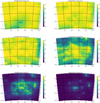 |
Fig. 2. Completeness maps for six bins at representative magnitudes. The completeness calculations have been smoothed with a Gaussian filter to ensure that at least three galaxies were used (within one sigma) to compute the completeness. |
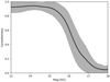 |
Fig. 3. Completeness as a function of R2 magnitude for each magnitude bin. The solid line corresponds to the mean, and the shaded region shows the standard deviation of the completeness across the studied catalogue area. |
7. Velocity distribution and structure of the SSC
The definition of the structure and topology of the SSC is not an easy task because of the complexity of the structures in the velocity distribution. The presence of many clusters, with their characteristic finger-of-God velocity structures, complicates the study in three dimensions. Moreover, remaining irregularities and gaps in the observations could mimic apparent structures. Finally, as modern redshift surveys show, dense structures are linked to each other by filaments and walls, forming a fabric that weaves throughout space.
7.1. Angular distribution
To improve our understanding of the matter distribution of the supercluster, we generated a three-dimensional density field in redshift-space. This was done using a three-dimensional Gaussian kernel in redshift-space and compensating by the completeness calculations described above. Each galaxy was assigned an individual kernel of the form
 (3)
(3)
were σa is the same angular kernel radius used in the completeness analysis and σv is the velocity dispersion fixed to 500 km s−1. The normalization ensures that each galaxy contributes with a single count when integrating over the full redshift-space volume, provided that σa and σv are small compared to the scales of interest. The density at each point of redshift-space is then computed by summing over the contributions of all galaxies, represented by these (properly shifted) density kernels, weighted by the inverse of the completeness associated with each galaxy. The units of the resulting density is counts per unit redshift-space volume. To equalise the pixel solid angles and produce a more physical representation of the density field, we used a flat projection of the sky coordinates onto a tangential plane centered at RA 13:29:36 and Dec −30:59:05.
Figure 4 shows a map of the projected density field of the SSC area. This was obtained by integrating our redshift-space density field in velocity, such that the units become counts per solid angle in arcminute squared. The integration ranged between 9000 and 18 000 km s−1, restricting to SSC relevant structures only. We note that the redshift-space density field does incorporate matter contributions from structure in front and behind this velocity range, as implied by the kernel in Eq. (3).
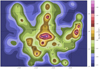 |
Fig. 4. Projected density field in the SSC area with velocities between 9000 and 18 000 km s−1. Known clusters between 8500 and 18 500 km s−1 are included for reference. |
7.2. Velocity distribution and structure of the supercluster
There are 10 702 galaxies in total, but the importance of the SSC in this region of the sky is demonstrated by the fact that approximately 5600 (52%) of the galaxies belong to the SSC and its immediate neighbourhood, if we consider as such all galaxies with velocities in the range 9000–18 000 km s−1 (a total depth of 90 h−1 Mpc). It can be seen that by probing large regions of the SSC away from the richer Abell clusters, we have confirmed significant structures which make links with the main cluster.
From the density plot and the velocity distribution, we can infer some features of the three-dimensional structure of the supercluster, taking due consideration of the abundant presence of fingers of god in this dense volume. Figure 5 shows the histogram of the velocities of galaxies in the direction of the SSC with all available velocities in the range 0 ≤ v≤ 30 000 km s−1, with a step size of 300 km s−1. The histogram shows several maxima, as discussed by Quintana et al. (2000) and Proust et al. (2006). Figure 6 shows the combined resulting distribution of galaxies towards the SSC as wedge diagrams in Right Ascension (left) and Declination (right) of the whole velocity catalogue until 30 000 km s−1. Figure 7 is a similar plot that provides a closer look are the SSC region, limited between 9000 km s−1 and 18 000 km s−1, revealing the rich interconnected structure within the central parts and to their neighbouring closer concentrations.
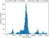 |
Fig. 5. Histogram of galaxy velocities in the direction of the SSC with all velocities available in the range 0 ≤ v ≤ 30 000 km s−1, with a step size of 300 km s−1. |
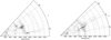 |
Fig. 6. Projections in RA (left) and Dec (right) of the distribution of galaxies with measured redshifts in the region of the SSC until 30 000 km s−1. The angle in Right Ascension is expanded by a factor of 2 and in Declination by a factor of 3 relative to its true size for clarity. |
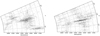 |
Fig. 7. Projections in RA (left) and Dec (right) of the distribution of galaxies with measured redshifts in the region of the SSC with velocities between 9000 and 18 000 km s−1. The angle in declination is expanded by a factor of 1.5 relative to its true size for clarity. |
The prominent foreground wall of galaxies (Hydra-Centaurus region) is defined centered close to 4200 km s−1. A second foreground structure at approximately 7200 km s−1 is composed of galaxies forming a tail between the Hydra-Centaurus and SSC regions, as can be seen in the Wedge diagrams of Fig. 6. The main body of the SSC is represented by the highest peak of 4600 galaxies, which is centered at approximately 15 000 km s−1. A few low relative peaks centered between 10 000 km s−1 and 13 000 km s−1, forming a sort of plateau in the histogram, shows the nearer concentration which is located to the East, centered on A3571, and connected to the main SSC body, as shown in Fig. 7.
The larger velocity catalogue used here confirms the general structure and the main features of the SSC already discussed in Quintana et al. (2000) and Proust et al. (2006). For completeness we briefly summarise them here. The central region is roughly spherical in shape centered on the cluster A3558, and has at its core the highest-density, elongated volume containing the Abell clusters A3562, A3558, and A3556, with almost identical recession velocities around 14 400 km s−1, and the groups SC1329-314 (Melnick & Moles 1987; Quintana et al. 1995) and SC1327-312 (Breen et al. 1994; Quintana et al. 1995), whose more discrepant velocities (by several hundred kilometers per second) could be attributed to the in-fall component along the line of sight. Towards the south of the elongated feature, the central region contains also the cluster A3560. As described in Reisenegger et al. (2000), the whole of this central region and all of its immediate surroundings are within the volume that is currently undergoing gravitational collapse. As shown in Fig. 6, we note the presence of the prominent foreground wall of galaxies of the Hydra-Centaurus region. Moreover, the “Front Eastern Wall” (Quintana et al. 2000), composed of a bridge of galaxies, groups and clusters, extends to the east and in front of the supercluster, the densest part being at ≃10 000–11 000 km s−1, located to the east. It contains the clusters A3571, A3572, and A3575 and the group SC1336-314 (Proust et al. 2006). The A3570 cluster is located at the southern tip of the observed part of the wall, and A3578 at its northern one. This wall establishes a further link between the Hydra-Centaurus region and the SSC, while a second one extends towards the west at  . Clumps of objects clearly link the two main structures. However, care must be taken in the interpretation of the wedge plots because of the finger-of-God effect evident in the main SSC concentrations (made especially prominent by the higher completeness in these cluster regions) and because of an analogous effect with opposite sign due to the inflow on larger scales, which makes the overdensities appear more overdense in redshift space than they are in the real space.
West and slightly North of the SSC core, another rich concentration of galaxies is connected to the central SSC regions. The clusters A3528, A3530, and A3532 form a concentration of galaxies and clusters at about RA = 12h50m and v = 16 000 − 17 000 km s−1 connected to the main body of the SSC by a broad bridge of galaxies. It can also be seen from the wedge diagram in declination (Fig. 7) that the southern part of the SSC consists of several clouds of galaxies where the known Abell clusters represent the peaks of maximum density. In this diagram, the sheet at  is present right across the observed region from −23° to −38°, which corresponds to the long complex of galaxies as shown on the Fig. 9 of the 6dF survey (Jones et al. 2009). We note that the central region of the SSC, with 11 clusters and groups (A3552, A3554, A3556, A3558, A3559, A3560, A3562, AS0724, AS0726, SC1327-312, and SC1329-314 [also named as SC1329-313]) has also been analysed by Haines et al. (2018), leading to similar conclusions. They give evidence that A3560 has two distinct sub-structures within r200, one to the north and one to the west, and its connecting structure is NW towards A3558.
In their supercluster catalogue, Einasto et al. (2001), applying a friends-of-friends algorithm, define a larger SSC (# 124), which includes two farther extensions (outside our survey area). To the North, one includes A1631, A1644, and A1709, reaching up to Dec −15°, while a Southern one, including A3548, A3561, and A3563 (none with measured redshifts, according to the NED database), reaches down to Dec −44°. Certainly, future velocity surveys could explore these areas to find out whether the SSC is even larger than measured so far.
8. Conclusions
We present a catalogue containing 18 129 velocities for 10 702 galaxies in the area of the SSC by combining existing measurements from the literature with 5084 new velocities for 2585 new galaxies observed by us at LCO and CTIO. The objects were cross-matched with galaxies from the SuperCOSMOS Sky Surveys to incorporate proper photometry and astrometry to the velocity measurements. This compilation of catalogues from various authors resolves several issues that we encountered, like coordinate misprints, zero-point velocity corrections, and cross-matching identification errors, resulting in a clean catalogue for scientific use. We provide the catalogue together with a completeness estimation as function of magnitude and position on the sky across most of the catalogue area.
By adding velocity measurements covering areas between known clusters, we improved our understanding of filaments connecting the central clusters, revealing a complicated structure of gravitationally interacting elements. These elements are yet to be proven gravitationally bound, an analysis that we are leaving for a future publication. The extended catalogue also reveals the possible existence of several new groups and poor cluster candidates, also allowing to test the reality of some proposed structures, which will also be explored in a future study.
Las Campanas Observatory (LCO) is an astronomical observatory owned and operated by the Carnegie Institution for Science (CIS).
Cerro Tololo Inter-American Observatory is operated by the Associations of Universities for Research in Astronomy under contract with the National Science Foundation.
The NASA/IPAC Extragalactic Database is operated by the Jet Propulsion Laboratory, California Institute of Technology, under contract with the National Aeronautics and Space Administration.
This long work was carried out by one of us (HQ) over parts of several years. It was done in two main periods, first for the central area and then an enlarged area by adding two strips of 5 deg at the N and S borders.
This is the case for the following references: Bade et al. (1995), Bernardi et al. (2002), Crook et al. (2007), Doyle et al. (2005), Fairall et al. (1992), Francis et al. (2004), Hickson et al. (1992), Jones et al. (2004), Lauberts & Valentjin (1989), Lavaud & Hudson (2011), Huchtmeier et al. (2005), Lawrence et al. (1999), Lipari et al. (1991), Maia et al. (1993), Mathewson et al. (1992), Mathewson & Ford (1996), Matthews & Gallagher (1996), Mauch & Sadler (2007), Maza & Ruiz (1989), Monnier Ragaigne et al. (2003), Paturel et al. (2003), Richter (1984), Scarpa et al. (1996), Schindler (2000), Zaritsky et al. (1997).
Acknowledgments
HQ is grateful to LCO and CTIO for generous allocations of telescope time. DP thanks the Instituto de Astrofísica of Pontificia Universidad Católica de Chile and ESO in the context of the Visiting Scientists program for their hospitality in Santiago (Chile). RD and AR acknowledge support from CONICYT project Basal AFB-170002 (CATA). This research has made use of data obtained from the SuperCOSMOS Science Archive, prepared and hosted by the Wide Field Astronomy Unit, Institute for Astronomy, University of Edinburgh, which is funded by the UK Science and Technology Facilities Council. We also thank the referee for useful comments.
References
- Abell, G. O., Corwin, H. G., & Olowin, R. P. 1989, ApJS, 70, 1 [NASA ADS] [CrossRef] [EDP Sciences] [Google Scholar]
- Allen, D. A., Norris, R. P., Meadows, V. S., & Roche, P. F. 1991, MNRAS, 248, 528 [Google Scholar]
- Araya-Melo, P. A., Reisenegger, A., Meza, A., et al. 2009, MNRAS, 399, 97 [Google Scholar]
- Bade, N., Fink, H. H., Engels, D., et al. 1995, A&AS, 110, 469 [NASA ADS] [Google Scholar]
- Bardelli, S., Zucca, E., Vettolani, G., et al. 1994, MNRAS, 267, 665 [Google Scholar]
- Bardelli, S., Zucca, E., Vettolani, G., Zamorani, G., & Scaramella, R. 1997, ApL&C, 36, 251 [NASA ADS] [Google Scholar]
- Bardelli, S., Zucca, E., Zamorani, G., Vettolani, G., & Scaramella, R. 1998a, MNRAS, 296, 599 [NASA ADS] [CrossRef] [Google Scholar]
- Bardelli, S., Pisani, A., Ramella, M., Zucca, E., & Zamorani, G. 1998b, MNRAS, 300, 589 [Google Scholar]
- Bardelli, S., Zucca, E., Zamorani, G., Moscardini, L., & Scaramella, R. 2000, MNRAS, 312, 540 [NASA ADS] [CrossRef] [Google Scholar]
- Bardelli, S., Zucca, E., & Baldi, A. 2001, MNRAS, 320, 387 [Google Scholar]
- Bernardi, M., Alonso, M. V., Da Costa, L. N., et al. 2002, AJ, 123, 2990 [NASA ADS] [CrossRef] [Google Scholar]
- Breen, J., Raychaudhury, S., Forman, W., & Jones, C. 1994, ApJ, 424, 59 [NASA ADS] [CrossRef] [Google Scholar]
- Cava, A., Bettoni, D., Poggianti, B. M., et al. 2009, A&A, 495, 707 [NASA ADS] [CrossRef] [EDP Sciences] [Google Scholar]
- Chiueh, T., & He, X.-G. 2002, PhRvD, 65, 123518 [Google Scholar]
- Chon, G., Böhringer, H., & Nowak, N. 2013, MNRAS, 429, 3272 [NASA ADS] [CrossRef] [Google Scholar]
- Chon, G., Böhringer, H., & Zaroubi, S. 2015, A&A, 575, L14 [NASA ADS] [CrossRef] [EDP Sciences] [Google Scholar]
- Cristiani, S., de Souza, R., D’Odorico, S., Lund, G., & Quintana, H. 1987, A&A, 179, 108 [NASA ADS] [Google Scholar]
- Crook, A. C., Huchra, J. P., Martimbeau, N., et al. 2007, ApJ, 655, 790 [NASA ADS] [CrossRef] [Google Scholar]
- da Costa, L. N., Nunes, M. A., Pellegrini, P. S., et al. 1986, AJ, 91, 6 [NASA ADS] [CrossRef] [Google Scholar]
- da Costa, L. N., Willmer, C., Pellegrini, P. S., & Chincarini, G. 1987, AJ, 93, 1338 [NASA ADS] [CrossRef] [Google Scholar]
- da Costa, L. N., Willmer, C. N. A., Pellegrini, P. S., et al. 1998, AJ, 116, 1 [Google Scholar]
- Dale, D. A., Giovanelli, R., Haynes, M. P., Hardy, E., & Campusano, L. E. 1999, AJ, 118, 1468 [NASA ADS] [CrossRef] [EDP Sciences] [Google Scholar]
- de Souza, R. E., de Melo, D. F., & Dos Anjos, S. 1997, A&AS, 125, 329 [Google Scholar]
- Doyle, M. T., Drinkwater, M. J., Rohde, D. J., et al. 2005, MNRAS, 361, 34 [NASA ADS] [CrossRef] [MathSciNet] [Google Scholar]
- Dressler, A. 1991, ApJS, 75, 241 [NASA ADS] [CrossRef] [Google Scholar]
- Dressler, A., & Shectman, S. 1988, AJ, 95, 284 [NASA ADS] [CrossRef] [Google Scholar]
- Drinkwater, M. J., Proust, D., Parker, Q. A., Quintana, H., & Slezak, E. 1999, PASA, 16, 113 [Google Scholar]
- Drinkwater, M. J., Parker, Q. A., Proust, D., Slezak, E., & Quintana, H. 2004, PASA, 21, 89 [NASA ADS] [CrossRef] [Google Scholar]
- Dünner, R., Araya, P. A., Meza, A., & Reisenegger, A. 2006, MNRAS, 366, 803 [NASA ADS] [CrossRef] [Google Scholar]
- Einasto, M., Einasto, J., Tago, E., Müller, V., & Andernach, H. 2001, AJ, 122, 2222 [CrossRef] [Google Scholar]
- Einasto, J., Hutsi, G., Einasto, M., et al. 2003a, A&A, 405, 425 [NASA ADS] [CrossRef] [EDP Sciences] [Google Scholar]
- Einasto, J., Einasto, M., Hutsi, G., et al. 2003b, A&A, 410, 425 [NASA ADS] [CrossRef] [EDP Sciences] [Google Scholar]
- Fairall, A. P., Willmer, C. N. A., Calderon, J. H., et al. 1992, AJ, 103, 11 [Google Scholar]
- Francis, P. J., Nelson, B. O., & Cutri, R. M. 2004, AJ, 127, 646 [NASA ADS] [CrossRef] [Google Scholar]
- Garcia, A. M., Bottinelli, L., Garnier, R., Gouguenheim, L., & Paturel, G. 1994, A&AS, 107, 265 [NASA ADS] [Google Scholar]
- Haines, C. P., Busarello, G. P., Merluzzi, P., et al. 2018, MNRAS, 481, 1055 [Google Scholar]
- Hickson, P., Mendes de Oliveira, C., & Huchra, J. P. 1992, ApJ, 399, 353 [NASA ADS] [CrossRef] [EDP Sciences] [MathSciNet] [PubMed] [Google Scholar]
- Hoffman, Y., Pomarede, D., Tully, R. B., & Courtois, H. 2017, Nat. Astron., 1, 0036 [NASA ADS] [CrossRef] [Google Scholar]
- Huchra, J. P., Macri, L. M., Masters, K. L., et al. 2012, ApJS, 199, 26 [NASA ADS] [CrossRef] [Google Scholar]
- Huchtmeier, W. K., Karachentsev, I. D., Karachenseva, V. E., Kudrya, Yu. N., & Mitronova, S. N. 2005, A&A, 435, 459 [NASA ADS] [CrossRef] [EDP Sciences] [Google Scholar]
- Jones, D. H., Saunders, W., Colless, M., et al. 2004, MNRAS, 355, 747 [NASA ADS] [CrossRef] [Google Scholar]
- Jones, D. H., Read, M. A., Saunders, W., et al. 2009, MNRAS, 399, 683 [NASA ADS] [CrossRef] [Google Scholar]
- Jorgensen, I., Franx, M., & Kjaergaard, P. 1995, MNRAS, 276, 1341 [NASA ADS] [Google Scholar]
- Kaldare, R., Colless, M., Raychaudhury, S., & Peterson, B. A. 2003, MNRAS, 339, 652 [NASA ADS] [CrossRef] [Google Scholar]
- Katgert, P., Mazure, A., & den Hartog, R. 1998, A&AS, 129, 399 [Google Scholar]
- Kocevski, D. D., Mullis, C. R., & Ebeling, H. 2004, ApJ, 608, 721 [NASA ADS] [CrossRef] [Google Scholar]
- Koribalski, B. S., Staveley-Smith, L., Kilborn, V. A., et al. 2004, AJ, 128, 16 [NASA ADS] [CrossRef] [Google Scholar]
- Kuntschner, H., Smith, R. J., Colless, M., et al. 2002, MNRAS, 337, 172 [NASA ADS] [CrossRef] [Google Scholar]
- Lauberts, A., & Valentjin, E. A. 1989, "The Surface Photometry Catalogue of the ESO-Uppsala (Galaxies", ESO) [Google Scholar]
- Lauer, T. R., Postman, M., Strauss, M. A., Graves, G. J., & Chisari, N. E. 2014, ApJ, 797, 82 [Google Scholar]
- Lavaud, G., & Hudson, M. J. 2011, MNRAS, 416, 2840 [NASA ADS] [CrossRef] [Google Scholar]
- Lawrence, A., Rowan-Robinson, M., Ellis, R. S., et al. 1999, MNRAS, 308, 897 [NASA ADS] [CrossRef] [Google Scholar]
- Lipari, S., Bonatto, C., & Pastoriza, M. G. 1991, MNRAS, 253, 19 [Google Scholar]
- Maia, M. A. G., da Costa, L. N., Giovanelli, R., & Haynes, M. P. 1993, AJ, 105, 2107 [NASA ADS] [CrossRef] [EDP Sciences] [Google Scholar]
- Maia, M. A. G., Suzuki, J. A., da Costa, L. N., Willmer, C. N. A., &Rite, C. 1996, A&AS, 117, 487 [Google Scholar]
- Masters, K. L., Crook, A., Hong, T., et al. 2014, MNRAS, 443, 1144 [Google Scholar]
- Mathewson, D. S., & Ford, V. L. 1996, ApJS, 107, 97 [NASA ADS] [CrossRef] [Google Scholar]
- Mathewson, D. S., Ford, V. L., & Buchhorn, M. 1992, ApJS, 81, 413 [NASA ADS] [CrossRef] [Google Scholar]
- Matthews, L. D., & Gallagher, J. S., III 1996, AJ, 111, 1098 [Google Scholar]
- Mauch, T., & Sadler, E. M. 2007, MNRAS, 375, 931 [NASA ADS] [CrossRef] [Google Scholar]
- Maza, J., & Ruiz, M. T. 1989, ApJS, 69, 353 [NASA ADS] [CrossRef] [Google Scholar]
- Melnick, J., & Moles, M. 1987, Rev. Mex. A&A, 14, 72 [NASA ADS] [Google Scholar]
- Melnick, J., & Quintana, H. 1981, A&AS, 44, 87 [NASA ADS] [Google Scholar]
- Merluzzi, P., Busarello, G., Dopita, M. A., et al. 2013, MNRAS, 429, 1747 [NASA ADS] [CrossRef] [Google Scholar]
- Merluzzi, P., Busarello, G., Dopita, M. A., et al. 2016, MNRAS, 460, 3345 [Google Scholar]
- Metcalfe, N., Godwin, J. G., & Spencer, S. D. 1987, MNRAS, 225, 581 [NASA ADS] [CrossRef] [EDP Sciences] [Google Scholar]
- Meyer, M. J., Zwaan, M. A., Webster, R. L., et al. 2004, MNRAS, 350, 1195 [NASA ADS] [CrossRef] [Google Scholar]
- Momcheva, I. G., Williams, K. A., Cool, R. J., Keeton, C. R., & Zabludoff, A. I. 2015, ApJS, 219, 1 [Google Scholar]
- Monnier Ragaigne, D., van Driel, W., Schneider, S. E., Balkowski, C., & Jarrett, T. H. 2003, A&A, 408, 465 [Google Scholar]
- Ogando, R. L., Maia, M. A. G., Pellegrini, P. S., & da Costa, L. N. 2008, AJ, 135, 2424 [NASA ADS] [CrossRef] [Google Scholar]
- Paturel, G., Theureau, G., Bottinelli, L., et al. 2003, A&A, 412, 57 [NASA ADS] [CrossRef] [EDP Sciences] [Google Scholar]
- Pimbblet, K. A., Smail, I., Edge, A. C., et al. 2006, MNRAS, 366, 645 [NASA ADS] [CrossRef] [Google Scholar]
- Postman, M., & Lauer, T. R. 1995, ApJ, 440, 28 [NASA ADS] [CrossRef] [Google Scholar]
- Proust, D., Quintana, H., Carrasco, E. R., et al. 2006, A&A, 447, 133 [NASA ADS] [CrossRef] [EDP Sciences] [Google Scholar]
- Quintana, H., & de Souza, R. 1993, A&AS, 101, 475 [NASA ADS] [Google Scholar]
- Quintana, H., Ramirez, A., Melnick, J., Raychaudhury, S., & Slezak, E. 1995, AJ, 110, 463 [NASA ADS] [CrossRef] [EDP Sciences] [Google Scholar]
- Quintana, H., Melnick, J., Proust, D., & Infante, L. 1997, A&AS, 125, 247 [Google Scholar]
- Quintana, H., Carrasco, E. R., & Reisenegger, A. 2000, AJ, 120, 511 [NASA ADS] [CrossRef] [Google Scholar]
- Raychaudhury, S. 1989, Nature, 342, 251 [Google Scholar]
- Reisenegger, A., Quintana, H., Carrasco, E. R., & Maze, J. 2000, AJ, 120, 523 [Google Scholar]
- Richter, O. G. 1984, A&AS, 58, 131 [NASA ADS] [Google Scholar]
- Richter, O. G. 1987, A&AS, 67, 261 [NASA ADS] [Google Scholar]
- Scaramella, R., Baiesi-Pillastrini, G., Chincarini, G., Vettolani, G., & Zamorani, G. 1989, Nature, 338, 562 [NASA ADS] [CrossRef] [EDP Sciences] [Google Scholar]
- Scarpa, R., Falomo, R., & Pesce, J. E. 1996, A&AS, 116, 295 [Google Scholar]
- Schindler, S. 2000, A&AS, 142, 433 [NASA ADS] [CrossRef] [EDP Sciences] [Google Scholar]
- Shapley, H. 1930, Harv. Coll. Obs. Bull., 874, 9 [NASA ADS] [Google Scholar]
- Shectman, S. A. 1989, Year Book 89 (Washington: Carnegie, Inst.), 25 [Google Scholar]
- Sheth, R. K., & Diaferio, A. 2011, MNRAS, 417, 2938 [Google Scholar]
- Smith, R. J., Lucey, J. R., Hudson, M. J., Schlegel, D. J., & Davies, R. L. 2000, MNRAS, 313, 469 [NASA ADS] [CrossRef] [Google Scholar]
- Smith, R. J., Hudson, M. J., Nelan, J. E., et al. 2004, AJ, 128, 1558 [NASA ADS] [CrossRef] [Google Scholar]
- Smith, R. S., Lucey, J. R., & Hudson, M. J. 2007, MNRAS, 381, 1035 [NASA ADS] [CrossRef] [EDP Sciences] [Google Scholar]
- Stein, P. 1996, A&AS, 116, 203 [Google Scholar]
- Strauss, M. A., Huchra, J. P., Davis, M., et al. 1992, ApJS, 83, 29 [NASA ADS] [CrossRef] [EDP Sciences] [Google Scholar]
- Surace, C., & Comte, G. 1998, A&AS, 133, 171 [Google Scholar]
- Teague, P. F., Carter, D., & Gray, P. M. 1990, ApJS, 72, 715 [NASA ADS] [CrossRef] [Google Scholar]
- Theureau, G., Bottinelli, L., Coudreau-Durand, N., et al. 1998, A&AS, 130, 133 [Google Scholar]
- Theureau, G., Hanski, M. O., Coudreau, N., Hallet, N., & Martin, J. M. 2007, A&A, 465, 71 [NASA ADS] [CrossRef] [EDP Sciences] [Google Scholar]
- Tonry, J., & Davis, M. 1979, AJ, 84, 1511 [NASA ADS] [CrossRef] [Google Scholar]
- Tully, B. R., Courtois, H., Hoffman, Y., & Pomarede, D. 2014, Nature, 513, 71 [NASA ADS] [CrossRef] [Google Scholar]
- Vettolani, G., Chincarini, G., Scaramella, R., & Zamorani, G. 1990, AJ, 99, 1709 [Google Scholar]
- Wegner, G., Bernardi, M., Willmer, C. N. A., et al. 2003, AJ, 126, 2268 [NASA ADS] [CrossRef] [Google Scholar]
- Willmer, C. N. A., Focardi, P., Chan, R., Pellegrini, P. S., & da Costa, L. N. 1991, AJ, 101, 57 [NASA ADS] [CrossRef] [Google Scholar]
- Willmer, C. N. A., Maia, M. A. G., Mendes, S. O., et al. 1999, AJ, 118, 1131 [Google Scholar]
- Zaritsky, D., Smith, R., Frenk, C., & White, S. D. M. 1997, ApJ, 478, 39 [NASA ADS] [CrossRef] [Google Scholar]
Appendix A: HI velocity measurements and possible wrong or confused identifications
We found a number of velocity and/or positional discrepancies between optical and HI measurements. For these cases there are three possible explanations: (a) the optical velocity is wrong due a number of factors, either misprints, wrong identification of the galaxy at the telescope, or just a wrong velocity determination (a blunder). (b) the HI velocity is the result of a confusion or reflection from other sources in the beam. (c) Since the HI positions are uncertain typically between 1′ − 2′, and up to 6′ (see HIPASS optical catalogue, HOPCAT, Doyle et al. 2005), there could be a wrong identification of the HI source. When there are two or more consistent and independent optical velocities, the possibilities are reduced to b or c. Therefore, the correct identification is given by the position of the galaxy image used for the optical velocity determination.
One factor affecting the reliability of the identifications is caused by the allocation of the HI velocity to a bright galaxy near the HI position, which is identified with the source. Different catalogues have adopted this practice (FLASH, NED, Simbad, possibly ZCAT, and others), without keeping the original HI pointing coordinates (sometimes, these are unpublished). Furthermore, due to the small velocity errors of the HI measurements, these velocities are selected by previous catalogues as the most precise z values.
In this Appendix we discuss eight cases of discrepant HI vs. optical velocities, with comments concerning possible identification alternatives. Two galaxies, ESO 507-036 and IC4254, have optical redshifts that place them in the SSC velocity range, farther away than normally listed.
ESO 381-020, a low-surface-brightness (disaggregated) Irr galaxy. Data is #22 in Database (and comments). NED and other catalogues give a low z derived from HI velocities. Problem: Dr91 gives 3399 km s−1, while Ka03 (source ZCAT from HI data) and Ko04 (HIPASS) give 585 km s−1, discrepant velocities from Dr91. All 3 have positions consistent with ESO381-020. The velocity quoted by Ka03 may not be an independent measurement. The SuperCOSMOS galaxy image has morphology consistent with v≈600 km s−1. Its large angular extension means the 3 positions are spread over the central very irregular area. There are no other nearby Sp or Irr galaxies within 15′. Either the Dr91 measurement is faulty, or the Dr91 velocity corresponds to a background galaxy, hard to distinguish among irregularities of the main lsb Irr galaxy image.
ESO 507-036, an Sp galaxy. Data is #8461 in Database (and comments). The 6dFGS survey gives a velocity of 13 803 km s−1 and a well-centered position on the Sp nucleus. Huchtmeier et al. (2005, Hu05) gives an HI value of 3364 km s−1 with a position within the optical edge-on Sp image. Another 6dFGS Sp at 13 551 km s−1 is located ≈5.5′ to the north. Both publications give the coordinates of the ESO galaxy, with highly discrepant velocities, but 6dFGS is an exact direct coordinate measurement. The SuperCOSMOS optical image of the edge-on spiral suggests a warp of the main disk with a hotspot, or maybe it is a possible background, also edge-on, spiral aligned with the main disk. However, the most likely option is that the Hu05 value is a velocity of a different Sp, as there are several smaller spirals within 5′, and there is another edge-on Sp with 3000 km s−1 at ≈20′ to the SE.
ESO 443-059, a bright spiral. Data is #1472 in Database (and comments). Three optical velocities (6dFGS, Dr91, Da87) and one HI (Maia et al. 1996, Ma96 in NED) are consistent at ≈3400 km s−1 and consistent with the ESO443-059 position. Problem: the FLASH survey Ka03 quotes a NED HI source that gives 2293 km s−1. The discrepant FLASH velocity indicates a wrong id for the HI source. Most likely the source could be identified with Database #1492 Sp at ≈3′ to the NE, which has 3 velocity measurements around 2310 km s−1. Alternatively, but less likely, the Ka03 velocity could be identified with #1507 with v = 2266 (velocity from Ba97) located ≈9′ away to the NE. Both are likely members of a group around nearby NGC 4965 at ≈2300 km s−1.
ESO 443-061, a spiral. Data is #1504 in Database (and comments). There are two independent and consistent optical velocities (6dFGS and LC97) at ≈9500 km s−1. The Ko04 HIPASS brightest-1000 survey measures a velocity of 2282 km s−1 from a position 5′15″ away from this galaxy. NED and others assign this Ko04 HI velocity to ESO 443-061, which is a wrong optical identification. The HIPASS velocity is consistent with some NGC 4965 group members. Alternatively, it could be a rare HI cloud, or another galaxy. In fact, the most likely identification for this HIPASS source is with #1507 from our Database. At 2′10″ this is closer to the HIPASS position than to ESO 443-061.
IC 4254 a bright peculiar galaxy. Data is #3681 in Database (and comments). Two optical, independent and consistent velocities (Dr88, St96) give ≃15 350 km s−1 and make it a likely member of the A1736 cluster (old velocity NED value used by Ka03). However, HI observations at Nançay (The98) give a velocity of 3503 km s−1. Problem: The98, NED, and many catalogues give IC4254 the low z, but the optical distance is ≈5 times higher, in a rich cluster within the SSC. Alternative identifications for the Nançay The98 observation: few nearby galaxies are without velocity measurements (the field is that of the A1736 cluster). Possibilities are an Sp 2′20′ to N (at 13 27 44.11 −27 11 03.3; R2 = 16.47), though it looks distant, and, more likely, an lsb Irr gal 4′10′ to NW (at 13 27 30.03 −27 10 27.5; R2 = 16.8)
ESO 444-082. Data is #5238 in Database (and comments). With three consistent positions, a very low HI Nançay velocity of ≈526 km s−1 is given by The98, while two independent consistent (QC03, 6dFGS) optical measurements give a value ≈11 300 km s−1. NED and others chose the low z from The98, which in view of the optical data looks like a wrong identification or poor data. It is unclear if the Nançay position is just that of the optical image, with an erroneous identification. Alternatives: No obvious candidate within 10’. No obvious explanation. Perhaps confused HI data.
NGC 5298, a bright Sp. Data is #6234 in Database (and comments). Nançay The98 HI velocity at 4083 km s−1 and identification (Ka03). Four optical velocities (LC97, Dr91, Da87, and 6dFGS) and one HI velocity (Mathewson et al. 1992, Ma92) are consistent at ≈4400 km s−1, and the position is in A3574 cluster field, at similar z (4400 km s−1). However, the velocity observed by Nançay (The98) has a discrepancy of 350 km s−1, quite significant for an HI measurement. It seems the galaxy identification could be misplaced, as there are a few surrounding spirals with closer velocities to The98 4083 km s−1: closest is 1′ to N.
Galaxy L606P Sp. HI Nançay (Monnier Ragaigne et al. 2003, Mon03) gives a 541 km s−1 velocity and identification. Data is #6839 in Database (and comments). There is a 6dFGS optical velocity measured of 3778 km s−1 of this fairly small Sp. Several nearby galaxies have similar z, which is of cluster S0753. The Nançay 541 km s−1 low velocity (it should be a very near galaxy), is discrepant value to 6dFGS. Several surrounding brighter galaxies at 3800–4400 km s−1 (in S0753). No likely candidate within 15′. It could be a confused source or an HI cloud.
All Tables
Zero-point corrections for each of the surveys included in our database with respect to our reference set.
All Figures
|
Fig. 1. Spectroscopic survey fields reported in this paper. Large squares are LCO fiber spectrograph observations. Circles are Hydra fields observed at CTIO, and small blue squares are WFCCD fields observed at LCO. The area of this plot is smaller than the total catalogue area, chosen to zoom in on the surveyed fields. The gray dots represent the positions of all galaxies in the velocity catalogue. Red dots are the positions of those galaxies whose velocities were measured by our group and reported in this paper. |
| In the text | |
|
Fig. 2. Completeness maps for six bins at representative magnitudes. The completeness calculations have been smoothed with a Gaussian filter to ensure that at least three galaxies were used (within one sigma) to compute the completeness. |
| In the text | |
|
Fig. 3. Completeness as a function of R2 magnitude for each magnitude bin. The solid line corresponds to the mean, and the shaded region shows the standard deviation of the completeness across the studied catalogue area. |
| In the text | |
|
Fig. 4. Projected density field in the SSC area with velocities between 9000 and 18 000 km s−1. Known clusters between 8500 and 18 500 km s−1 are included for reference. |
| In the text | |
|
Fig. 5. Histogram of galaxy velocities in the direction of the SSC with all velocities available in the range 0 ≤ v ≤ 30 000 km s−1, with a step size of 300 km s−1. |
| In the text | |
|
Fig. 6. Projections in RA (left) and Dec (right) of the distribution of galaxies with measured redshifts in the region of the SSC until 30 000 km s−1. The angle in Right Ascension is expanded by a factor of 2 and in Declination by a factor of 3 relative to its true size for clarity. |
| In the text | |
|
Fig. 7. Projections in RA (left) and Dec (right) of the distribution of galaxies with measured redshifts in the region of the SSC with velocities between 9000 and 18 000 km s−1. The angle in declination is expanded by a factor of 1.5 relative to its true size for clarity. |
| In the text | |
Current usage metrics show cumulative count of Article Views (full-text article views including HTML views, PDF and ePub downloads, according to the available data) and Abstracts Views on Vision4Press platform.
Data correspond to usage on the plateform after 2015. The current usage metrics is available 48-96 hours after online publication and is updated daily on week days.
Initial download of the metrics may take a while.