| Issue |
A&A
Volume 638, June 2020
The XXL Survey: third series
|
|
|---|---|---|
| Article Number | A45 | |
| Number of page(s) | 33 | |
| Section | Extragalactic astronomy | |
| DOI | https://doi.org/10.1051/0004-6361/201937161 | |
| Published online | 09 June 2020 | |
The XXL Survey
XL. Obscuration properties of red AGNs in XXL-N
1
National Observatory of Athens, V. Paulou & I. Metaxa, 15 236 Penteli, Greece
e-mail: This email address is being protected from spambots. You need JavaScript enabled to view it.
2
Section of Astrophysics, Astronomy and Mechanics, Department of Physics, Aristotle University of Thessaloniki, 54 124 Thessaloniki, Greece
3
Instituto de Fisica de Cantabria (CSIC-Universidad de Cantabria), Avenida de los Castros, 39005 Santander, Spain
4
Dipartimento di Fisica e Astronomia, Alma Mater Studiorum, Universitá degli Studi di Bologna, Via Gobetti 93/2, 40129 Bologna, Italy
5
INAF – Osservatorio di Astrofisica e Scienza dello Spazio di Bologna, Via Gobetti 93/3, 40129 Bologna, Italy
6
AIM, CEA, CNRS, Université Paris-Saclay, Université Paris Diderot, Sorbonne Paris Cité, 91191 Gif-sur-Yvette, France
7
INAF, IASF Milano, Via Corti 12, 20133 Milano, Italy
8
Centre for Extragalactic Astronomy, Department of Physics, Durham University, Durham DH1 3LE, UK
9
Department of Astronomy, University of Geneva, Ch. d’Écogia 16, 1290 Versoix, Switzerland
Received:
21
November
2019
Accepted:
9
March
2020
Abstract
The combination of optical and mid-infrared (MIR) photometry has been extensively used to select red active galactic nuclei (AGNs). Our aim is to explore the obscuration properties of these red AGNs with both X-ray spectroscopy and spectral energy distributions (SEDs). In this study, we re-visit the relation between optical/MIR extinction and X-ray absorption. We use IR selection criteria, specifically the W1 and W2 WISE bands, to identify 4798 AGNs in the XMM-XXL area (∼25 deg2). Application of optical/MIR colours (r−W2 > 6) reveals 561 red AGNs (14%). Of these, 47 have available X-ray spectra with at least 50 net (background-subtracted) counts per detector. For these sources, we construct SEDs from the optical to the MIR using the CIGALE code. The SED fitting shows that 44 of these latter 47 sources present clear signs of obscuration based on the AGN emission and the estimated inclination angle. Fitting the SED also reveals ten systems (∼20%) which are dominated by the galaxy. In these cases, the red colours are attributed to the host galaxy rather than AGN absorption. Excluding these ten systems from our sample and applying X-ray spectral fitting analysis shows that up to 76% (28/37) of the IR red AGNs present signs of X-ray absorption. Thus, there are nine sources (∼20% of the sample) that although optically red, are not substantially X-ray absorbed. Approximately 50% of these sources present broad emission lines in their optical spectra. We suggest that the reason for this apparent discrepancy is that the r−W2 criterion is sensitive to smaller amounts of obscuration relative to the X-ray spectroscopy. In conclusion, it appears that the majority of red AGNs present considerable obscuration levels as shown by their SEDs. Their X-ray absorption is moderate with a mean of NH ∼ 1022 cm−2.
Key words: galaxies: active / X-rays: galaxies
© ESO 2020
1. Introduction
The vast majority of galaxies host a supermassive black hole (SMBH) in their centre (e.g. Kormendy et al. 1996a,b). The masses of these SMBHs range from hundreds of thousands to billions of solar masses (≈105 − 1010 M⊙). When a SMBH grows, it releases huge amounts of energy across the electromagnetic spectrum and becomes visible as an AGN. These latter objects have characteristic properties such as high luminosities (up to Lbol ≃ 1048 erg s−1) and rapid variability (e.g. Ulrich et al. 1997).
According to the unification scheme (Antonucci 1993) the central source of the AGN structure consists of the SMBH, the corona, and the accretion disc. These regions are surrounded by an axisymmetric dusty structure that is toroidal in shape (e.g. Netzer 2015). Starting from the inner part of the source, the X-ray and the optical/ultraviolet (UV) wavelengths are related to the corona and the accretion disc respectively (e.g. Wilkins & Gallo 2015; Haardt & Maraschi 1991). The torus is responsible for the infrared (IR) emission (e.g. Edelson & Malkan 1986), because the hot dust is related to the radiation at these wavelengths. There are different torus models based on the distribution of dust, such as smooth (e.g. Fritz et al. 2006), clumpy (Nenkova et al. 2008a,b; Hönig & Kishimoto 2010, 2017; Hönig et al. 2010), and a combination of the two (Siebenmorgen et al. 2015; Stalevski et al. 2016). Unified models propose that the different observational classes of AGNs are nevertheless a single type of physical object observed at different viewing angles (e.g. different orientations of the observer with respect to the torus). Thus, Type 1 and Type 2 AGNs refer to the face-on (unobscured) and edge-on (obscured) AGNs, respectively. However, in the case of a clumpy torus, the classification of AGN type is not necessarily a consequence of a difference in viewing angle, because the dust is not distributed homogeneously. Based on their optical/UV spectrum, Type 1 AGNs present broad permitted emission lines, while Type 2 objects show only narrow lines. There is a continuum of objects in between (intermediate types), where the broad line components are increasingly difficult to observe.
Despite the huge radiative power of AGNs, obscuration presents an important challenge for uncovering their complete population and explaining the complicated mechanisms that regulate these systems (Hickox & Alexander 2018). Regarding the different obscuring material, X-ray energies are obscured by gas, whereas UV, optical, and IR wavelengths are extincted by dust. A reliable method to identify and quantify obscuration is through X-ray observations. Modelling of the X-ray spectrum provides a robust estimation of the NH column density.
The combination of optical and IR data also provides us with a powerful tool to search for obscured AGNs. The optical emission of a SMBH is attenuated by dust and is re-emitted in the NIR to MIR wavelengths. In this case the galaxy appears faint in the optical but bright in the IR (LaMassa et al. 2016). Various optical and IR colour criteria have been used in the literature to identify red AGNs, using either Spitzer (e.g. Fiore et al. 2009; Hickox et al. 2007; LaMassa et al. 2016; Donoso et al. 2014) or WISE (Yan et al. 2013) IR bands.
Previous studies have found a correlation between the optical/IR colours and X-ray absorption (e.g. Civano et al. 2012). On the other hand, Koutoulidis et al. (2018) found that reddened AGNs are equally divided into X-ray absorbed and unabsorbed. Specifically, these latter authors used about 1500 X-ray AGNs from five deep Chandra fields (CDF-N, CDF-S, ECDF-S, COSMOS, AEGIS) and divided them into obscured and unobscured sources using X-ray (Hardness Ratio) and optical/mid-infrared (MIR) criteria (R − [4.5] = 6.1). Nevertheless their sources span low luminosities (1042 − 1043 erg s−1). Based on their findings Koutoulidis et al. suggested that host galaxy contamination in the MIR bands affects the optical/MIR AGN classification.
We examine whether or not red AGNs are also absorbed in X-rays. To this aim, we use X-ray AGNs in the XXL survey (Pierre et al. 2016, hereafter XXL paper I) and select IR AGN candidates by applying the criteria of Assef et al. (2018). We use optical and MIR colours (Yan et al. 2013) to select optically red sources. The final sample is restricted to those AGNs for which X-ray spectroscopy is available (47 sources). In Sect. 3.1 we fit the X-ray spectra to quantify the X-ray absorption of the sources. In addition we construct spectral energy distributions (SEDs) using optical, near-infrared (NIR), and MIR photometry. We use the CIGALE code (Ciesla et al. 2015) to fit the SEDs and get an estimation of various absorption indices (AGN emission, torus inclination). We also complement our analysis with available optical spectra (see Sect. 3.3). Finally, we compare the results of different wavelengths and techniques for each red AGN.
2. Data
The data of this study come from the XXL survey. In this section we describe the survey as well as the sample selection.
2.1. XXL
The XXL survey is a medium-depth X-ray survey that covers a total area of 50 deg2. It covers two fields of nearly equal size, the XXL North (XXL-N) and the XXL South (XXL-S). Furthermore, it is the largest XMM-Newton project approved to date (> 6 Ms) with median exposure at 10.4 ks and a depth of ∼6 × 10⁻¹⁵ erg s−1 cm−2 for point sources at the 90% completeness limit in the [0.5−2] keV band (XXL paper I). In this study, we use the XXL-N sample that consists of 14 168 sources, including extended objects. To identify the X-ray detections at other wavelengths the X-ray counterparts have been crossmatched with optical, NIR, and MIR surveys (for more details see Chiappetti et al. 2018, hereafter XXL paper XXVII).
2.2. Infrared AGN candidates
WISE (Wright et al. 2010) completed an all-sky coverage in four MIR bands: 3.4, 4.6, 12, and 22 μm (W1, W2, W3 and W4 bands, respectively). Various colour criteria used these IR bands to efficiently identify AGN candidates. For instance, Mateos et al. (2012) suggested a selection method using three WISE colours. Stern et al. (2012) used the W1 and W2 bands and applied the criterion W1 − W2 ≥ 0.8 to select AGNs with W2 < 15.05 in the COSMOS field. Assef et al. (2013) extended the latter criterion and provided a selection of AGNs for fainter WISE sources using the WISE All-Sky data release catalogue. Assef et al. (2018) modified these criteria to incorporate data obtained during the post-cryogenic main mission extension (AllWISE catalogue).
In this study, we use approximately 500 000 WISE detections included in the latest WISE catalogue (AllWISE) that lie within the XMM-XXL area to select IR AGN candidates, applying the criteria of Assef et al. (2018). Specifically, we use
 (1)
(1)
![Mathematical equation: $$ \begin{aligned} W1-W2&> \alpha _R\,\exp \,[{\beta _{R}\,{(W2 - \gamma _{R})}^2}], \;\; W2 > \gamma _{R}, \end{aligned} $$](/articles/aa/full_html/2020/06/aa37161-19/aa37161-19-eq2.gif) (2)
(2)
where (αR, βR, γR) = (0.650, 0.153, 13.86), to select AGNs with 90% reliability.
2.3. Red AGNs
To select optically red sources from the IR AGN candidates, we apply the Yan et al. (2013) criterion (r−W2 > 6). This analysis reveals 561 red AGNs. We cross-match this subsample with the XXL catalogue to identify the X-ray counterparts of these sources. For the cross-match, we use a radius of 3 arcsec. Within this radius and given the X-ray source sky density, we find that a fraction of ∼0.2% of spurious matches is expected (Mountrichas et al. 2017). To study the X-ray absorption of the optically red AGN population, we apply an X-ray spectral fitting analysis. As one of our main goals is to quantify the obscuration in the red AGNs, we chose to analyse only the X-ray spectra of the sources with reliable photon statistics. For this reason, we keep only the sources with 50 or more net counts per detector (see Corral et al. 2015). There are 47 red AGNs that meet the aforementioned X-ray criteria. Table 1 presents the number of sources in the various subsamples. Table 2 presents the identity (ID), the redshift, and the r and W2 magnitudes in the Vega system for the 47 optically red AGNs. In addition to optical and MIR photometry, 45 out of the 47 optically red AGNs have also been detected in the NIR (VISTA; Emerson et al. 2006; Dalton et al. 2006). The XXL field has been observed by the SPIRE instrument onboard Herschel mission at far-infrared (FIR) wavelengths (Oliver 2012). To identify the FIR counterparts, we used the ARCHES cross-correlation tool XMATCH (Pineau et al. 2017). The details of the cross-match procedure are given in Sect. 2.2 of Masoura et al. (2018). We find nine sources with Herschel photometry. Finally, optical spectra are available for 33 out of the 47 red AGNs. The vast majority of them (30 out of 33) come from the SDSS (DR15) survey. The remaining optical spectra are from the Galaxy And Mass Assembly (GAMA; Driver et al. 2011; Baldry et al. 2010) and the VIPERS (Guzzo et al. 2014; Scodeggio et al. 2018) surveys. In our analysis, we use spectroscopic redshifts for 33 sources. For the remaining AGNs we use their photometric redshifts, estimated in Fotopoulou et al. (2016, hereafter XXL paper VI). The photometric redshift accuracy is 0.095 (for the full XMM-XXL catalogue). In our analysis, we incorporate the full probability density function (PDF) of the photometric redshifts when we calculate the uncertainties of the various parameters.
Number of IR-selected AGNs with X-ray and optical observations and spectra in the XMM-XXL field.
General properties of the red AGN sample.
3. Analysis
We classify the 47 optically red AGNs of our sample as obscured or unobscured using different criteria. Specifically, we examine their X-ray spectra, SEDs, and optical spectra.
3.1. X-ray spectra
We examine the X-ray absorption of the 47 red AGNs in our sample. To achieve that, we apply X-ray spectral-fitting using the XSPEC v12.10 software (Arnaud 1996). We use the Cash statistical analysis (C-stat; Cash 1979) on the spectra binned to 1 count/bin, which has been shown to recover the actual spectral parameters in the most accurate way even for very low-count spectra (e.g. Krumpe et al. 2008). The model applied to the spectral data is a simple power law, A(E) = KE−Γ, absorbed by both the Galactic photoelectric absorption and the intrinsic absorption. Γ is the photon index of the power law and K is the flux at 1 keV in units of photons keV−1 cm−2 s−1. The Galactic absorption is taken from the Leiden/Argentine/Bonn (LAB) Survey of Galactic HI Kalberla et al. (2005). The X-ray spectra for the 47 AGNs are presented in Figs. A.1–A.47. The best-fit values are presented in Table 3. In Fig. 1 we present NH versus X-ray luminosity.
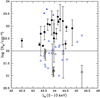 |
Fig. 1. NH as a function of X-ray luminosity for the 47 optical red AGNs. Those sources for which the X-ray spectral fitting could not constrain their NH are presented with a triangle (upper limit estimations). The 21 AGNs that satisfy our X-ray absorption criteria are presented with filled symbols (see text for more details). |
X-ray properties of the red AGN sample.
Figure 2 presents the NH distribution of the sources, taking into account the NH upper limits (Isobe et al. 1986). For that purpose, we use the Astronomical SURVival Statistics (ASURV; Lavalley et al. 1992) software package, which adopts the maximum-likelihood Kaplan-Meier estimator to take into account censored data (Feigelson & Nelson 1985). The derived mean value is log NH/cm−2 = 21.80 ± 0.13. The distribution shows that the red sources are almost equally divided between obscured (NH > 1022 cm−2) and unobscured AGNs. The limit of NH = 1022 cm−2 is often used in X-rays because lower column densities can be produced by dust lanes in the galaxy instead of the torus (Malkan et al. 1998). However, we note that Merloni et al. (2013) propose an alternative dividing line of 3 × 1021 cm−2 in the sense that this provides a much better agreement when compared with the optical classification between Type-1 and Type-2 AGNs. From Figs. 1 and 2 it appears that the red r−W2 colour alone cannot guarantee that the source will be classified as obscured in X-rays.
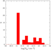 |
Fig. 2. NH distribution taking into account NH upper limits; see text for more details. |
3.2. SED fitting
We calculate the contribution of the AGNs to the power output of the host galaxy using the Code Investigating GALaxy Emission (CIGALE; Burgarella et al. 2005; Noll et al. 2009). We provide the CIGALE code version 2018.0 with multi-wavelength flux densities, using optical, NIR, and MIR photometry. Table 4 presents the models and the parameters used by CIGALE for the SED fitting of our X-ray sample. The Fritz et al. (2006) library of templates was used to model the AGN emission. The AGN fraction is measured as the AGN emission relative to IR luminosity (1−1000 μm). Here, τ is the e-folding time of the main stellar population model in millions of years. Age is defined as the age of the main stellar population, also in millions of years. The extinction of a source is derived from the viewing angle, Ψ, of the torus: Ψ ≤ 30° for Type 2 (edge-on), 40° ≤Ψ = 60° for intermediate, and Ψ ≥ 70° for Type 1 AGNs (face-on; Ciesla et al. 2015), respectively. No intermediate values are used. The results from these fits appear in Table 5 and the SEDs are shown in Figs. A.1–A.47 (for more details on the SED fitting, see also Masoura et al. 2018).
Models and values for their free parameters used by CIGALE for the SED fitting of our X-ray samples.
SED properties of the red AGN sample.
As mentioned in the previous section, Herschel photometry is available for nine of the sources in our sample. We fit the SEDs of these sources with and without FIR data to check whether the lack of FIR photometric bands affects the SED fitting measurements. Specifically, we are interested in the inclination angle Ψ, since this parameter is used as a proxy to determine the obscuration of an AGN. We find that the inclusion of FIR photometry in the SED fitting does not change the AGN emission or the estimated inclination angle of the sources. Thus, we conclude that a lack of FIR photometry for the remaining sources does not affect our analysis.
3.3. Optical spectra
The optical spectra for 33 out of 47 sources are presented in Figs. A.1–A.47. Optically unobscured sources (Type 1) are considered to be those with broad emission lines (BL), whereas obscured sources (Type 2) exhibit only narrow emission lines (NL) or a red continuum. The AGNs are characterised as obscured, unobscured, or intermediate (IMD) type, based on visual inspection of their optical spectra. Table 6 contains the classification according to the optical spectrum for each object.
Optical properties of the red AGN sample.
To verify the redshift of our sources and assess their obscuration in the optical band we used the optical spectra provided by the SDSS. We recomputed the spectroscopic redshift and for a small number of cases we provide in Table 2 a different measurement from the one in SDSS.
4. Discussion
Our IR selection criteria identify 4798 AGN candidates (Table 1). Of these, 2652 have been observed by SDSS. Approximately 20% of these sources are optically red using the criteria of Yan et al. (2013); see Table 1. Figures 3 and 4 show the i-band and the r−W2 distributions of the various samples. As expected, red sources occupy the faint part of the i-band distribution while the AGN sample with available X-ray spectra lacks sources with the highest r−W2 values.
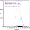 |
Fig. 3. i-band distribution of our sample. Red sources occupy the faint part of the i-band distribution. |
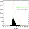 |
Fig. 4. r−W2 distribution of our sample. The AGN sample with available X-ray spectra lacks sources with the highest r−W2 values. |
In our analysis, we explore the X-ray spectral properties of the 47 optically red AGNs and examine whether these sources are also X-ray absorbed. Furthermore, we search for indications of extinction either on their SEDs or in their optical spectra. The results of the X-ray spectral fitting are presented in Table 3. For those cases where the photon index (Γ) is unphysically low (Γ < 1.2) we quote the NH estimations with Γ fixed to Γ = 1.8 (Nandra & Pounds 1994). The latter NH estimation is used to characterise the X-ray absorption of the source. Our analysis reveals 18 sources with best-fit intrinsic column densities NH > 1022 cm−2. We also consider as possibly absorbed a source whose upper limit lies above the arbitrary chosen limit of NH = 1023 cm−2 (i.e. J020543.0−051656, J020953.9−055102, J021509.0−054305). The latter increases the number of candidate X-ray-absorbed sources to 21. We characterise these systems as X-ray-absorbed sources and mark them in bold in Table 7. However, there are AGNs that present mild absorption and could be classified as X-ray absorbed if we eased our X-ray criteria. Thus, lowering our X-ray absorption criteria, that is, NH > 1021.5 cm−2 (Merloni et al. 2013) or upper limit that lies above the NH value NH = 1022 cm−2, we find 13 additional sources that present signs of X-ray absorption. These additional sources are shown in italics in Table 7. Therefore, up to 34 AGNs (72%) in the sample present some signs of X-ray absorption.
Comparison of the X-ray, SED, and optical properties.
The vast majority of our optically red AGNs have SEDs that show clear signs of obscuration in their AGN emission (green lines is Figs. A.1–A.47). However, the AGN emission of the source J022809.0−041235 (no. 4 in Table 5) extends to the optical part of the spectrum without presenting signs of even mild obscuration. This source has also large Ψ (Ψ = 80°) that also indicates a Type 1 AGN (X-ray and optical spectra also confirm this is an unobscured AGN). There are two more sources with a large Ψ value (i.e. observed face-on), namely sources J020517.3−051024 and J021808.8−055630 (nos. 11 and 28 in Table 5). Their SEDs reveal that even though the AGN emission extends to the optical part of the SED, the emission of the galaxy is a dominant component of the SED at the optical wavelengths. We refer to the latter two systems as galaxy dominated. We attribute this term to sources that satisfy the following criteria: (i) the IR (W2) emission of the system is due to the AGN emission, and (ii) there is a strong galaxy emission in the optical part of the SED even though the AGN emission is only mildly obscured (or not obscured at all). Specifically, the ratio of the galaxy emission to the AGN emission in the r band is ≥1. Although source no. 28 is not X-ray absorbed, source no. 11 presents signs of mild X-ray absorption ( cm−2). The optical spectra of these two systems have broad emission lines, corroborating the assertion that these are unobscured sources. We conclude that the SEDs for 44 out of the 47 sources in our sample present clear signs of obscuration based on their AGN emission and their Ψ values.
In addition to these two AGNs (i.e. sources 11 and 28 in Table 5), there are eight more sources that satisfy our aforementioned criteria and are therefore considered galaxy-dominated systems (nos. 5, 7, 10, 26, 35, 39, 44, and 47). In these systems, the galaxy and/or AGN emission in the r band ranges from ≈1 (e.g. no. 28) to ≥10 (e.g. nos. 10, 39, and 47). Five of these sources are among the AGNs that are also X-ray absorbed (nos. 10, 26, 35, 39, and 47 in Table 7). Their AGN fraction, fracAGN = 40−80% (Table 5). These suggest that these systems are galaxy dominated because the AGN is obscured and not because the active SMBH is intrinsically weak. However, for the remaining three galaxy-dominated systems (nos. 5, 7, and 44) that are not X-ray absorbed, it could be that they are characterised as optically red (r−W2 > 6) due to an intrinsically weak AGN (AGN fraction, fracAGN = 20−30%, Table 5) rather than an obscured AGN. Galaxy-dominated systems are known to confuse optical and MIR criteria (Koutoulidis et al. 2018).
Excluding the ten galaxy-dominated systems from our sample of red IR AGNs reduces the total number of red sources to 37. Of these, 17 (46% of the total sample) and 28 (76% of the total sample) are X-ray absorbed using the strict and loose criteria, respectively. Therefore, there are nine (∼20%) IR red AGNs in our sample that present no signs of X-ray absorption. The optical spectra for two of these sources present narrow emission lines (nos. 16 and 20 in Table 7), four present broad emission lines (nos. 1, 3, 9, and 25 in Table 7) and two are of intermediate type (nos. 17 and 18 in Table 7) based on our visual inspection. The optical spectrum of source no. 23 is too noisy to extract any information. Previous studies have found that selection of obscured AGNs based on optical and/or MIR colours are 80% reliable (Hickox et al. 2007). This could explain why at least some of these nine AGNs, although optically red, present broad emission lines in their spectra and no substantial X-ray absorption.
Recently, Jaffarian & Gaskell (2020) studied the optical E(B − V) reddening versus the X-ray absorbing column density for a large sample of Seyfert galaxies with both E(B − V) and X-ray absorption column density measurements. These latter authors find a significant correlation between E(B − V) and NH, albeit with a large scatter of ±dex, which they claim could be attributed to X-ray column density variability. Regardless of the origin of the physical interpretation, the presence of such a large scatter can readily explain why some of our red sources show no sign of significant absorption in X-rays. The fact that the average absorbing column density derived for the red r−W2 > 6 sources is only NH = 21.8 ± 0.13 suggests that the above obscuration criterion selects sources with lower absorption compared to those selected in X-rays using NH > 1022 cm−2 (e.g. Akylas et al. 2006; Ueda et al. 2014). In other words, the optically red source selection does not correspond to the same level of obscuring column densities as those seen for X-ray wavelengths. Hickox et al. (2017) proposed an additional criterion for the selection of obscured AGNs based on the combination of the u and WISE W3 band. Since there is not a unique definition of how obscured an AGN must be to be classified as absorbed, the various selection criteria target different ranges of obscuration. Specifically, the application of the “usual” X-ray criterion NH > 1022 cm−2 selects the most obscured part of the obscured AGN distribution, while the r−W2 criterion extends to lower levels of obscuration. Finally, the Hickox et al. u–W3 criterion is sensitive to the lowest levels of obscuration. This is due to the use of the u band that is easily affected by even small amounts of reddening. The different selection criteria indeed result in different obscured AGN samples. This is most probably the reason why only 76% (at most) of the red AGN sample is absorbed in X-rays with column densities log NH/cm−2 > 21.5.
5. Summary
Here, we applied the Assef et al. (2018) criteria based on the W1 and W2 WISE bands to select IR AGNs in the XXL-North 25 deg2 survey area. The above criteria yield 4798 AGNs. Moreover, we applied the optical MIR colour criterion r−W2 (Yan et al. 2013) in order to select obscured AGNs. We identify 561 red AGNs, of which 135 are detected in X-rays while 47 have good photon statistics (at least 50 net counts per detector), and derive a reliable estimate of the absorbing column density. We used XSPEC to fit the X-ray spectra of the 47 sources and quantify their X-ray absorption. Of these 47 sources, 76% may show signs of absorption higher than log NH/cm−2 = 21.5. Furthermore, we applied the CIGALE code in order to study the SEDs of our 47 red sources. The SED analysis revealed that 10/47 sources are galaxy-dominated systems as the red colours are attributed to the host galaxy rather than absorption. In the vast majority of the remaining 37 sources, the SEDs confirm the presence of significant obscuration. The exact nature of the red sources that show low levels of X-ray absorption (25%) in apparent contradiction with their SEDs is unclear. The large scatter in the r−W2 colour versus column density, possibly caused by variability of the column density, is likely to offer an explanation. Our work shows that the r−W2 selection provides a robust method for selecting obscured AGNs. However, it may also identify sources that present lower levels of obscuration when compared with the widely used X-ray spectroscopic criteria which usually define obscured sources as those with log NH/cm−2 > 21.5.
Acknowledgments
The authors are grateful to the anonymous referee for helpful comments. VAM and GM acknowledge support of this work by the PROTEAS II project (MIS 5002515), which is implemented under the “Reinforcement of the Research and Innovation Infrastructure” action, funded by the “Competitiveness, Entrepreneurship and Innovation” operational programme (NSRF 2014−2020) and co-financed by Greece and the European Union (European Regional Development Fund). GM also acknowledges support by the Agencia Estatal de Investigación, Unidad de Excelencia María de Maeztu, Ref. MDM-2017-0765. The Saclay group acknowledges long-term support from the Centre National d’Etudes Spatiales (CNES). XXL is an international project based around an XXM Very Large Programme surveying two 25 deg2 extragalactic fields at a depth of ∼6 × 10⁻¹⁵ erg cm −2 s−1 in the [0.5−2] keV band forpoint-like sources. The XXL website is http://irfu.cea.fr/xxl/. Multi-band information and spectroscopic follow-up of the X-ray sources are obtained through a number of survey programmes, summarised at http://xxlmultiwave.pbworks.com/. This research has made use of data obtained from the 3XMM XMM-Newton serendipitous source catalogue compiled by the 10 institutes of the XMM-Newton Survey Science Centre selected by ESA. The Saclay group acknowledges long-term support from the Centre National d’Etudes Spatiales (CNES). This work is based on observations made with XMM-Newton, an ESA science mission with instruments and contributions directly funded by ESA Member States and NASA. Funding for the Sloan Digital Sky Survey IV has been provided by the Alfred P. Sloan Foundation, the US Department of Energy Office of Science, and the Participating Institutions. SDSS-IV acknowledges support and resources from the Center for High-Performance Computing at the University of Utah. The SDSS web site is www.sdss.org. SDSS-IV is managed by the Astrophysical Research Consortium for the Participating Institutions of the SDSS Collaboration including the Brazilian Participation Group, the Carnegie Institution for Science, Carnegie Mellon University, the Chilean Participation Group, the French Participation Group, Harvard-Smithsonian Center for Astrophysics, Instituto de Astrofísica de Canarias, The Johns Hopkins University, Kavli Institute for the Physics and Mathematics of the Universe (IPMU)/University of Tokyo, Lawrence Berkeley National Laboratory, Leibniz Institut für Astrophysik Potsdam (AIP), Max-Planck-Institut für Astronomie (MPIA Heidelberg), Max-Planck-Institut für Astrophysik (MPA Garching), Max-Planck-Institut für Extraterrestrische Physik (MPE), National Astronomical Observatories of China, New Mexico State University, New York University, University of Notre Dame, Observatário Nacional/MCTI, The Ohio State University, Pennsylvania State University, Shanghai Astronomical Observatory, United Kingdom Participation Group, Universidad Nacional Autónoma de México, University of Arizona, University of Colorado Boulder, University of Oxford, University of Portsmouth, University of Utah, University of Virginia, University of Washington, University of Wisconsin, Vanderbilt University, and Yale University. This publication makes use of data products from the Wide-field Infrared Survey Explorer, which is a joint project of the University of California, Los Angeles, and the Jet Propulsion Laboratory/California Institute of Technology, funded by the National Aeronautics and Space Administration. The VISTA Data Flow System pipeline processing and science archive are described in Irwin et al. (2004), Hambly et al. (2008) and Cross et al. (2012). Based on observations obtained as part of the VISTA Hemisphere Survey, ESO Program, 179.A-2010 (PI: McMahon). We have used data from the 3rd data release.
References
- Aguado, D. S., Hernández, J. I. G., Prieto, C. A., & Rebolo, R. 2019, ApJ, 874, L21 [NASA ADS] [CrossRef] [Google Scholar]
- Akylas, A., Georgantopoulos, I., Georgakakis, A., Kitsionas, S., & Hatziminaoglou, E. 2006, A&A, 459, 693 [NASA ADS] [CrossRef] [EDP Sciences] [Google Scholar]
- Antonucci, R. 1993, ARA&A, 31, 473 [Google Scholar]
- Arnaud, K. A. 1996, ASP Conf. Ser., 101, 17 [Google Scholar]
- Assef, R. J., Stern, D., Kochanek, C. S., et al. 2013, ApJ, 772, 26 [NASA ADS] [CrossRef] [Google Scholar]
- Assef, R. J., Stern, D., Noirot, G., et al. 2018, ApJS, 234, 23 [NASA ADS] [CrossRef] [Google Scholar]
- Baldry, I. K., Robotham, A. S. G., Hill, D. T., et al. 2010, MNRAS, 404, 86 [NASA ADS] [Google Scholar]
- Bruzual, G., & Charlotte, S. 2003, MNRAS, 344, 1000 [NASA ADS] [CrossRef] [Google Scholar]
- Burgarella, D., Buat, V., & Iglesias-Páramo, J. 2005, MNRAS, 360, 1413 [NASA ADS] [CrossRef] [Google Scholar]
- Calzetti, D., Armus, L., Bohlin, R. C., et al. 2000, ApJ, 533, 682 [NASA ADS] [CrossRef] [Google Scholar]
- Cash, W. 1979, ApJ, 228, 939 [NASA ADS] [CrossRef] [Google Scholar]
- Chiappetti, L., Fotopoulou, S., Lidman, C., et al. 2018, A&A, 620, A12 [NASA ADS] [CrossRef] [EDP Sciences] [Google Scholar]
- Ciesla, L., Charmandaris, V., Georgakakis, A., et al. 2015, A&A, 576, A10 [NASA ADS] [CrossRef] [EDP Sciences] [Google Scholar]
- Civano, F., Elvis, M., Brusa, M., et al. 2012, ApJS, 201, 30 [NASA ADS] [CrossRef] [Google Scholar]
- Corral, A., Georgantopoulos, I., Watson, M. G., et al. 2015, A&A, 576, A61 [NASA ADS] [CrossRef] [EDP Sciences] [Google Scholar]
- Cross, N. J. G., Collins, R. S., Mann, R. G., et al. 2012, A&A, 548, A119 [NASA ADS] [CrossRef] [EDP Sciences] [Google Scholar]
- Dalton, G. B., Caldwell, M., Ward, A. K., et al. 2006, Proc. SPIE, 6269, 62690X [CrossRef] [Google Scholar]
- Donoso, E., Yan, L., Stern, D., & Assef, R. J. 2014, ApJ, 789, 44 [NASA ADS] [CrossRef] [Google Scholar]
- Driver, S. P., Hill, D. T., Kelvin, L. S., et al. 2011, MNRAS, 413, 971 [NASA ADS] [CrossRef] [Google Scholar]
- Edelson, R. A., & Malkan, M. A. 1986, ApJ, 308, 59 [NASA ADS] [CrossRef] [Google Scholar]
- Emerson, J., McPherson, A., & Sutherland, W. 2006, The Messenger, 126, 41 [NASA ADS] [Google Scholar]
- Feigelson, E. D., & Nelson, P. I. 1985, ApJ, 293, 192 [NASA ADS] [CrossRef] [Google Scholar]
- Fiore, F., Puccetti, S., Brusa, M., et al. 2009, ApJ, 693, 447 [NASA ADS] [CrossRef] [Google Scholar]
- Fotopoulou, S., Pacaud, F., Paltani, S., et al. 2016, A&A, 592, A5 [NASA ADS] [CrossRef] [EDP Sciences] [Google Scholar]
- Fritz, J., Franceschini, A., & Hatziminaoglou, E. 2006, MNRAS, 166, 767 [NASA ADS] [CrossRef] [Google Scholar]
- Guzzo, L., Scodeggio, M., Garilli, B., et al. 2014, A&A, 566, A108 [NASA ADS] [CrossRef] [EDP Sciences] [Google Scholar]
- Haardt, F., & Maraschi, L. 1991, ApJ, 380, L51 [NASA ADS] [CrossRef] [Google Scholar]
- Hambly, N. C., Collins, R. S., Cross, N. J. G., et al. 2008, MNRAS, 384, 637 [NASA ADS] [CrossRef] [Google Scholar]
- Hickox, R., & Alexander, D. 2018, ARA&A, 56, 625 [Google Scholar]
- Hickox, R. C., Jones, C., Forman, W. R., et al. 2007, ApJ, 671, 1365 [NASA ADS] [CrossRef] [Google Scholar]
- Hickox, R. C., Myers, A. D., Greene, J. E., et al. 2017, ApJ, 849, 53 [NASA ADS] [CrossRef] [Google Scholar]
- Hönig, S. F., & Kishimoto, M. 2010, A&A, 523, A27 [NASA ADS] [CrossRef] [EDP Sciences] [Google Scholar]
- Hönig, S. F., & Kishimoto, M. 2017, ApJ, 838, L20 [NASA ADS] [CrossRef] [Google Scholar]
- Hönig, S. F., Kishimoto, M., Gandhi, P., et al. 2010, A&A, 515, A23 [NASA ADS] [CrossRef] [EDP Sciences] [Google Scholar]
- Irwin, M. J., Lewis, J., Hodgkin, S., et al. 2004, Optimizing Scientific Return for Astronomy through Information Technologies (SPIE), 5493 [Google Scholar]
- Isobe, T., Feigelson, E. D., & Nelson, P. I. 1986, ApJ, 306, 490 [NASA ADS] [CrossRef] [Google Scholar]
- Jaffarian, G. W., & Gaskell, C. M. 2020, MNRAS, 493, 930 [NASA ADS] [CrossRef] [Google Scholar]
- Kalberla, P. M. W., Burton, W. B., Hartmann, D., et al. 2005, A&A, 440, 775 [NASA ADS] [CrossRef] [EDP Sciences] [Google Scholar]
- Kormendy, J., Bender, R., Ajhar, E. A., et al. 1996a, ApJ, 473, L91 [NASA ADS] [CrossRef] [Google Scholar]
- Kormendy, J., Bender, R., Richstone, D., et al. 1996b, ApJ, 459, L57 [NASA ADS] [CrossRef] [Google Scholar]
- Koutoulidis, L., Georgantopoulos, I., Mountrichas, G., et al. 2018, MNRAS, 481, 3063 [NASA ADS] [CrossRef] [Google Scholar]
- Krumpe, M., Lamer, G., Corral, A., et al. 2008, A&A, 483, 415 [NASA ADS] [CrossRef] [EDP Sciences] [Google Scholar]
- LaMassa, S. M., Civano, F., Brusa, M., et al. 2016, ApJ, 818, 88 [NASA ADS] [CrossRef] [Google Scholar]
- Lavalley, M., Isobe, T., & Feigelson, E. 1992, ASP Conf. Ser., 25, 245 [NASA ADS] [Google Scholar]
- Malkan, M. A., Gorjian, V., & Tam, R. 1998, ApJS, 117, 25 [NASA ADS] [CrossRef] [Google Scholar]
- Masoura, V. A., Mountrichas, G., Georgantopoulos, I., et al. 2018, A&A, 618, A31 [NASA ADS] [CrossRef] [EDP Sciences] [Google Scholar]
- Mateos, S., Alonso-Herrero, A., Carrera, F. J., et al. 2012, MNRAS, 426, 3271 [NASA ADS] [CrossRef] [Google Scholar]
- Merloni, A., Bongiorno, A., Brusa, M., et al. 2013, MNRAS, 437, 3550 [Google Scholar]
- Mountrichas, G., Georgantopoulos, I., Secrest, N. J., et al. 2017, MNRAS, 468, 3042 [NASA ADS] [CrossRef] [Google Scholar]
- Nandra, K., & Pounds, K. A. 1994, MNRAS, 268, 405 [NASA ADS] [CrossRef] [Google Scholar]
- Nenkova, M., Sirocky, M. M., Nikutta, R., Ivezić, Ž., & Elitzur, M. 2008a, ApJ, 685, 160 [NASA ADS] [CrossRef] [Google Scholar]
- Nenkova, M., Sirocky, M. M., Ivezić, Ž., & Elitzur, M. 2008b, ApJ, 685, 147 [NASA ADS] [CrossRef] [Google Scholar]
- Netzer, H. 2015, ARA&A, 53, 365 [NASA ADS] [CrossRef] [Google Scholar]
- Noll, S., Burgarella, D., Giovannoli, E., et al. 2009, A&A, 507, 1793 [NASA ADS] [CrossRef] [EDP Sciences] [Google Scholar]
- Oliver, S. J., et al. 2012, MNRAS, 424, 1614 [NASA ADS] [CrossRef] [EDP Sciences] [Google Scholar]
- Pierre, M., Pacaud, F., Adami, C., et al. 2016, A&A, 592, A1 [NASA ADS] [CrossRef] [EDP Sciences] [Google Scholar]
- Pineau, F.-X., Derriere, S., Motch, C., et al. 2017, A&A, 597, A89 [NASA ADS] [CrossRef] [EDP Sciences] [Google Scholar]
- Scodeggio, M., Guzzo, L., Garilli, B., et al. 2018, A&A, 609, A84 [NASA ADS] [CrossRef] [EDP Sciences] [Google Scholar]
- Siebenmorgen, R., Heymann, F., & Efstathiou, A. 2015, A&A, 583, A120 [NASA ADS] [CrossRef] [EDP Sciences] [Google Scholar]
- Stalevski, M., Ricci, C., Ueda, Y., et al. 2016, MNRAS, 458, 2288 [NASA ADS] [CrossRef] [Google Scholar]
- Stern, D., Assef, R. J., Benford, D. J., et al. 2012, ApJ, 753, 30 [NASA ADS] [CrossRef] [Google Scholar]
- Ueda, Y., Akiyama, M., Hasinger, G., Miyaji, T., & Watson, M. G. 2014, ApJ, 786, 104 [NASA ADS] [CrossRef] [Google Scholar]
- Ulrich, M.-H., Maraschi, L., & Urry, C. M. 1997, ARA&A, 35, 445 [NASA ADS] [CrossRef] [Google Scholar]
- Wilkins, D. R., & Gallo, L. C. 2015, MNRAS, 448, 703 [NASA ADS] [CrossRef] [Google Scholar]
- Wright, E. L., Eisenhardt, P. R. M., Mainzer, A. K., et al. 2010, AJ, 140, 1868 [NASA ADS] [CrossRef] [Google Scholar]
- Yan, L., Donoso, E., Tsai, C.-W., et al. 2013, AJ, 145, 55 [NASA ADS] [CrossRef] [Google Scholar]
Appendix A: X-ray, optical spectra, and SEDs
In this section, we present the X-ray, SEDs, and the optical spectra (when available) for each one of the 47 optically red sources in our sample. Numbers 1 and 2 are used to denote the classification of the sources based on the various criteria. Specifically, 1 refers to unobscured and 2 to obscured sources. Number 0 is used in those cases where the optical spectrum is too noisy to extract any useful information. Number 3 is used to denote IMD type of classification. The numbers in parentheses refer to the classification based on the X-ray spectrum, the SED, and the optical spectrum, respectively. We use three decimal points for spectroscopic redshifts and two decimal points for photometric redshifts.
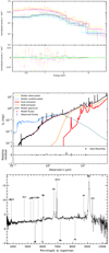 |
Fig. A.1. J021835.7−053758 (1,2,1), z = 0.387. |
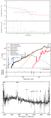 |
Fig. A.2. J022848.4−044426 (2,2,1), z = 1.046. |
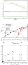 |
Fig. A.3. J022928.4−051124 (2,2,1), z = 0.307. |
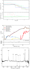 |
Fig. A.4. J022809.0−041235 (1,1,1), z = 0.879. |
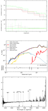 |
Fig. A.5. J020654.9−064552 (1,2,2), z = 1.412. |
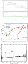 |
Fig. A.6. J020410.4−063924 (2,2,2), z = 0.414. |
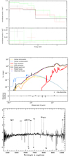 |
Fig. A.7. J023315.5−054747 (1,2,2), z = 0.598. |
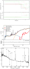 |
Fig. A.8. J021337.9−042814 (2,2,1), z = 0.419. |
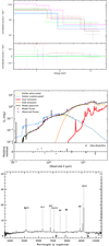 |
Fig. A.9. J020436.4−042833 (1,2,1), z = 0.827. |
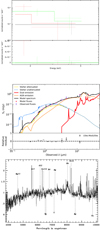 |
Fig. A.10. J020543.0−051656 (2,2,1), z = 0.653. |
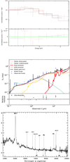 |
Fig. A.11. J020517.3−051024 (2,0,1), z = 0.792. |
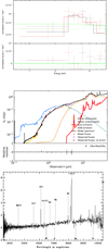 |
Fig. A.12. J022244.3−030525 (2,2,2), z = 0.637. |
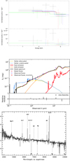 |
Fig. A.13. J022323.4−031157 (2,2,3), z = 0.691. |
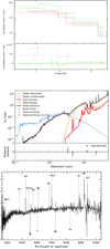 |
Fig. A.14. J022209.6−025023 (2,2,2), z = 0.400. |
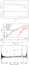 |
Fig. A.15. J022750.7−052232 (2,2,3), z = 0.804. |
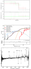 |
Fig. A.16. J022758.4−053306 (1,2,2), z = 0.956. |
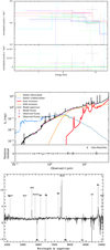 |
Fig. A.17. J022453.2−054050 (2,2,3), z = 0.488. |
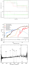 |
Fig. A.18. J022258.8−055757 (1,2,3), z = 0.732. |
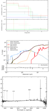 |
Fig. A.19. J021844.6−054054 (1,2,3), z = 0.671. |
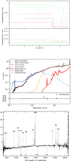 |
Fig. A.20. J021523.2−044337 (1,2,2), z = 0.860. |
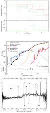 |
Fig. A.21. J022321.9−045739 (2,2,2), z = 0.779. |
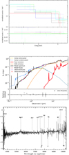 |
Fig. A.22. J022443.6−050905 (2,2,3), z = 0.943. |
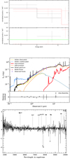 |
Fig. A.23. J023418.0−041833 (1,2,0), z = 0.582. |
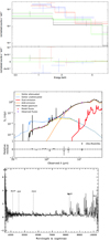 |
Fig. A.24. J020543.7−063807 (1,2,0), z = 0.772. |
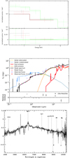 |
Fig. A.25. J022932.6−055438 (1,2,1), z = 1.263. |
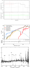 |
Fig. A.26. J021239.2−054816 (2,2,0), z = 0.711. |
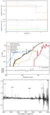 |
Fig. A.27. J021511.4−060805 (2,2,1), z = 0.772. |
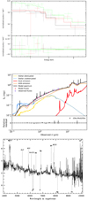 |
Fig. A.28. J021808.8−055630 (1,0,1), z = 0.572. |
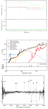 |
Fig. A.29. J022538.9−040821 (2,2,1), z = 0.733. |
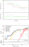 |
Fig. A.30. J020845.1−051354 (2,2), z = 1.46. |
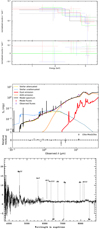 |
Fig. A.31. J020953.9−055102 (2,2,1), z = 0.642. |
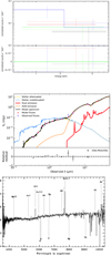 |
Fig. A.32. J020806.6−055739 (2,2,2), z = 0.539. |
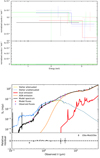 |
Fig. A.33. J021509.0−054305 (2,2), z = 0.70. |
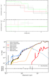 |
Fig. A.34. J021512.9−060558 (2,2), z = 1.14. |
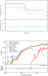 |
Fig. A.35. J020529.5−051100 (2,2), z = 1.20. |
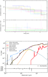 |
Fig. A.36. J022404.0−035730 (2,2), z = 0.17. |
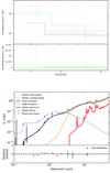 |
Fig. A.37. J023501.0−055234 (2,2), z = 0.85. |
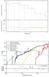 |
Fig. A.38. J020210.6−041129 (2,2), z = 2.71. |
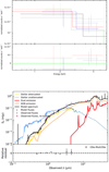 |
Fig. A.39. J022650.3−025752 (2,2), z = 1.21. |
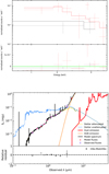 |
Fig. A.40. J021303.7−040704 (2,2), z = 1.35. |
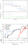 |
Fig. A.41. J023357.7−054819 (2,2), z = 1.60. |
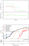 |
Fig. A.42. J020335.0−064450 (2,2), z = 0.67. |
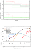 |
Fig. A.43. J020823.4−040652 (1,2), z = 2.23. |
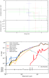 |
Fig. A.44. J020135.4−050847 (1,2), z = 0.73. |
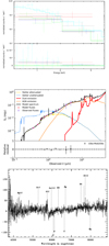 |
Fig. A.45. J021837.2−060654 (2,2,0), z = 0.943. |
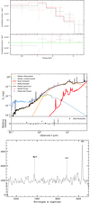 |
Fig. A.46. J022149.9−045920 (2,2,2), z = 1.461. |
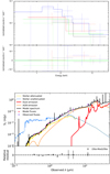 |
Fig. A.47. J020311.3−063534 (2,2), z = 1.05. |
All Tables
Number of IR-selected AGNs with X-ray and optical observations and spectra in the XMM-XXL field.
Models and values for their free parameters used by CIGALE for the SED fitting of our X-ray samples.
All Figures
|
Fig. 1. NH as a function of X-ray luminosity for the 47 optical red AGNs. Those sources for which the X-ray spectral fitting could not constrain their NH are presented with a triangle (upper limit estimations). The 21 AGNs that satisfy our X-ray absorption criteria are presented with filled symbols (see text for more details). |
| In the text | |
|
Fig. 2. NH distribution taking into account NH upper limits; see text for more details. |
| In the text | |
|
Fig. 3. i-band distribution of our sample. Red sources occupy the faint part of the i-band distribution. |
| In the text | |
|
Fig. 4. r−W2 distribution of our sample. The AGN sample with available X-ray spectra lacks sources with the highest r−W2 values. |
| In the text | |
|
Fig. A.1. J021835.7−053758 (1,2,1), z = 0.387. |
| In the text | |
|
Fig. A.2. J022848.4−044426 (2,2,1), z = 1.046. |
| In the text | |
|
Fig. A.3. J022928.4−051124 (2,2,1), z = 0.307. |
| In the text | |
|
Fig. A.4. J022809.0−041235 (1,1,1), z = 0.879. |
| In the text | |
|
Fig. A.5. J020654.9−064552 (1,2,2), z = 1.412. |
| In the text | |
|
Fig. A.6. J020410.4−063924 (2,2,2), z = 0.414. |
| In the text | |
|
Fig. A.7. J023315.5−054747 (1,2,2), z = 0.598. |
| In the text | |
|
Fig. A.8. J021337.9−042814 (2,2,1), z = 0.419. |
| In the text | |
|
Fig. A.9. J020436.4−042833 (1,2,1), z = 0.827. |
| In the text | |
|
Fig. A.10. J020543.0−051656 (2,2,1), z = 0.653. |
| In the text | |
|
Fig. A.11. J020517.3−051024 (2,0,1), z = 0.792. |
| In the text | |
|
Fig. A.12. J022244.3−030525 (2,2,2), z = 0.637. |
| In the text | |
|
Fig. A.13. J022323.4−031157 (2,2,3), z = 0.691. |
| In the text | |
|
Fig. A.14. J022209.6−025023 (2,2,2), z = 0.400. |
| In the text | |
|
Fig. A.15. J022750.7−052232 (2,2,3), z = 0.804. |
| In the text | |
|
Fig. A.16. J022758.4−053306 (1,2,2), z = 0.956. |
| In the text | |
|
Fig. A.17. J022453.2−054050 (2,2,3), z = 0.488. |
| In the text | |
|
Fig. A.18. J022258.8−055757 (1,2,3), z = 0.732. |
| In the text | |
|
Fig. A.19. J021844.6−054054 (1,2,3), z = 0.671. |
| In the text | |
|
Fig. A.20. J021523.2−044337 (1,2,2), z = 0.860. |
| In the text | |
|
Fig. A.21. J022321.9−045739 (2,2,2), z = 0.779. |
| In the text | |
|
Fig. A.22. J022443.6−050905 (2,2,3), z = 0.943. |
| In the text | |
|
Fig. A.23. J023418.0−041833 (1,2,0), z = 0.582. |
| In the text | |
|
Fig. A.24. J020543.7−063807 (1,2,0), z = 0.772. |
| In the text | |
|
Fig. A.25. J022932.6−055438 (1,2,1), z = 1.263. |
| In the text | |
|
Fig. A.26. J021239.2−054816 (2,2,0), z = 0.711. |
| In the text | |
|
Fig. A.27. J021511.4−060805 (2,2,1), z = 0.772. |
| In the text | |
|
Fig. A.28. J021808.8−055630 (1,0,1), z = 0.572. |
| In the text | |
|
Fig. A.29. J022538.9−040821 (2,2,1), z = 0.733. |
| In the text | |
|
Fig. A.30. J020845.1−051354 (2,2), z = 1.46. |
| In the text | |
|
Fig. A.31. J020953.9−055102 (2,2,1), z = 0.642. |
| In the text | |
|
Fig. A.32. J020806.6−055739 (2,2,2), z = 0.539. |
| In the text | |
|
Fig. A.33. J021509.0−054305 (2,2), z = 0.70. |
| In the text | |
|
Fig. A.34. J021512.9−060558 (2,2), z = 1.14. |
| In the text | |
|
Fig. A.35. J020529.5−051100 (2,2), z = 1.20. |
| In the text | |
|
Fig. A.36. J022404.0−035730 (2,2), z = 0.17. |
| In the text | |
|
Fig. A.37. J023501.0−055234 (2,2), z = 0.85. |
| In the text | |
|
Fig. A.38. J020210.6−041129 (2,2), z = 2.71. |
| In the text | |
|
Fig. A.39. J022650.3−025752 (2,2), z = 1.21. |
| In the text | |
|
Fig. A.40. J021303.7−040704 (2,2), z = 1.35. |
| In the text | |
|
Fig. A.41. J023357.7−054819 (2,2), z = 1.60. |
| In the text | |
|
Fig. A.42. J020335.0−064450 (2,2), z = 0.67. |
| In the text | |
|
Fig. A.43. J020823.4−040652 (1,2), z = 2.23. |
| In the text | |
|
Fig. A.44. J020135.4−050847 (1,2), z = 0.73. |
| In the text | |
|
Fig. A.45. J021837.2−060654 (2,2,0), z = 0.943. |
| In the text | |
|
Fig. A.46. J022149.9−045920 (2,2,2), z = 1.461. |
| In the text | |
|
Fig. A.47. J020311.3−063534 (2,2), z = 1.05. |
| In the text | |
Current usage metrics show cumulative count of Article Views (full-text article views including HTML views, PDF and ePub downloads, according to the available data) and Abstracts Views on Vision4Press platform.
Data correspond to usage on the plateform after 2015. The current usage metrics is available 48-96 hours after online publication and is updated daily on week days.
Initial download of the metrics may take a while.