| Issue |
A&A
Volume 638, June 2020
|
|
|---|---|---|
| Article Number | A147 | |
| Number of page(s) | 10 | |
| Section | Astrophysical processes | |
| DOI | https://doi.org/10.1051/0004-6361/201936740 | |
| Published online | 26 June 2020 | |
Fermi Large Area Telescope observations of the fast-dimming Crab Nebula in 60–600 MeV
Institute for Experimental Physics, Universität Hamburg, Luruper Chaussee 149, 22761 Hamburg, Germany
e-mail: kin.hang.yeung@desy.de
Received:
19
September
2019
Accepted:
5
May
2020
Context. The Crab pulsar and its nebula are the origin of relativistic electrons which can be observed through their synchrotron and inverse Compton emission. The transition between synchrotron-dominated and inverse-Compton-dominated emissions takes place at ≈109 eV.
Aims. The short-term (lasting for one week to months) flux variability of the synchrotron emission from the most energetic electrons is investigated with data from ten years of observations with the Fermi Large Area Telescope in the energy range from 60 MeV to 600 MeV.
Methods. We reconstructed the off-pulse light curve reconstructed from phase-resolved data. The corresponding histogram of flux measurements was used to identify distributions of flux-states and the statistical significance of a lower-flux component was estimated with dedicated simulations of mock light curves. The energy spectra for different flux states were also reconstructed.
Results. We confirm the presence of flaring-states which follow a log-normal flux distribution. Additionally, we discovered a low-flux state where the flux drops to as low as 18.4% of the intermediate-state average flux and remains there for several weeks. The transition time is observed to be as short as two days. The energy spectrum during the low-flux state resembles the extrapolation of the inverse-Compton spectrum measured at energies beyond several GeV energy, implying that the high-energy part of the synchrotron emission is dramatically depressed.
Conclusions. The low-flux state found here and the transition time of at most ten days indicate that the bulk (>75%) of the synchrotron emission above 108 eV originates in a compact volume with apparent angular size of θ ≈ 0″.4 tvar/(5 d). We tentatively infer that the so-called inner knot feature is the origin of the bulk of the γ-ray emission.
Key words: ISM: individual objects: Crab Nebula / gamma rays: ISM
© ESO 2020
1. Introduction
Isolated neutron stars and their environments are powerful sites of particle acceleration, which result in the formation of pulsar wind nebula (PWN) systems. In the case of the Crab Nebula, the extended cloud of non-thermal plasma is radiating in multi-wavelength, from radio to gamma-ray (Aharonian 2004; Bühler & Blandford 2014; Dubner et al. 2017).
The Crab Nebula is a PWN powered by a ∼1 kyr old pulsar (Hester 2008). It is a part of the core-collapse supernova remnant located in the constellation of Taurus and at a distance of 2 kpc (Trimble 1968). Due to the exceptionally wide observable energy range, we can study the processes of particle acceleration that are presumably happening at the termination shock and witness energy losses in the nebula (e.g., Spitkovsky & Arons 2004; Fraschetti & Pohl 2017).
The observed hard γ-ray (1 GeV–80 TeV) spectrum of the Crab Nebula has been compared with various model calculations which use widely different approaches (de Jager & Harding 1992; Atoyan & Aharonian 1996; Hillas et al. 1998; Volpi et al. 2008; Meyer et al. 2010; Martín et al. 2012). All these models assume that the gamma-ray emission in this energy range is predominantly produced via inverse-Compton (IC) scattering of relativistic electrons with synchrotron-radiated photons, as initially suggested by Rees (1971) and Gunn & Ostriker (1971).
Meanwhile, at lower energies, the observed nebular γ-ray (0.75 MeV–1 GeV) spectrum is presumably dominated by the synchrotron mechanism (Kuiper et al. 2001; Buehler et al. 2012). The Crab Nebula experiences recurrent flares (roughly one per year) detected with AGILE and Fermi Large Area Telescope (LAT), some of which boosted up the >100 MeV synchrotron flux by a factor of ≳20 (e.g., Tavani et al. 2011; Abdo et al. 2011; Buehler et al. 2012; Mayer et al. 2013). Enhanced γ-ray emission of the synchrotron component can last for a broad variety of timescales ranging from days to weeks (Striani et al. 2013). Ongoing instability of the synchrotron emission from the Crab Nebula is also observed in the hard X-ray/soft γ-ray regime over a longer range of time (Ling & Wheaton 2003; Wilson-Hodge et al. 2011).
In this work, we study the γ-ray variability of the Crab Nebula in detail, with the >60 MeV LAT data accumulated over about ten years during the off-pulse phase of the Crab pulsar. In addition to the flaring periods, we consider the entire light curve.
2. Data reduction and analysis
We performed a series of binned maximum-likelihood analyses (with an angular bin size of 0.1°) for a region of interest (ROI) of 30 ° ×30° centered at RA = 05h34m31.94s, Dec = +22 ° 00′52.2″ (J2000), which is approximately the center of the Crab Nebula (Lobanov et al. 2011). We use the data of 60 MeV–10 GeV photon energies, registered with the LAT between 2008 August 4 and 2018 August 20. The data were reduced and analyzed with the aid of the Fermi Science Tools v11r5p3 package.
Considering that the Crab Nebula is quite close to the Galactic plane (with a Galactic latitude of −5.7844°), we adopt the events classified as Pass8 “Clean” class for the analysis so as to better suppress the background. The corresponding instrument response function (IRF) “P8R2−CLEAN−V6” is used throughout the investigation. Only the data collected during the off-pulse phase (0.56–0.88; adopting the same convention of phase as in Buehler et al. 2012) of the Crab pulsar are selected for analysis. Correspondingly, a correction factor of 1/0.32 is taken into account in calculations of phase-averaged fluxes. We further filter the data by accepting only the good time intervals where the ROI was observed at a zenith angle less than 90° so as to reduce the contamination from the albedo of Earth.
In order to account for the contribution of diffuse background emission, we include the Galactic background (gll−iem−v06.fits), the isotropic background (iso−P8R2−CLEAN−V6−v06.txt), as well as all other point sources cataloged in the LAT 8-year Point Source Catalog (4FGL; The Fermi-LAT Collaboration 2019) within 32° from the ROI center in the source model. We set free the spectral parameters of the sources within 10° from the ROI center (including the prefactor and index of the Galactic diffuse background as well as the normalization of the isotropic background) in the analysis. For the sources at angular separation beyond 10° from the ROI center, their spectral parameters are fixed to the catalog values.
The three point sources located within the nebula are cataloged as 4FGL J0534.5+2200, 4FGL J0534.5+2201i, and 4FGL J0534.5+2201s, which respectively model the Crab pulsar, the IC, and synchrotron components of the Crab Nebula. We remove 4FGL J0534.5+2200 from the source model because the on-pulse data has been screened out. In broadband spectral analyses, we enable the energy dispersion correction which operates on the count spectra of most sources including the Crab Nebula, following the recommendations of the Fermi Science Support Center.
3. Spectral properties and variability of the Crab Nebula
3.1. Time-averaged spectrum
The energy spectrum of the off-pulse nebular component at energies between 60 MeV and 10 GeV is reconstructed using the combined observational data of approximately ten years (see previous section for an overview of the data reduction steps including the pulsar gating).
The data are fit by a two-component (additive) model. Similar to a previous study (Buehler et al. 2012), we use the superposition of a soft power law (PL) with a photon index constrained to the interval 3–5 for the synchrotron component and a hard PL with a photon index constrained within 0–2 for the IC component of the nebular emission. It is known that the spectrum of the IC component at energies beyond 10 GeV requires a more complex model. However, within our fitting range up to 10 GeV, two PL models are sufficient to characterize the broad-band spectrum (see Table 1 for the resulting parameters). More complex models including a “power law with exponential cutoff” (PLEC) for the synchrotron component are not significantly preferred, as a likelihood ratio test indicates that the improvement is not significant (∼1.3σ). It is comforting to see that the sum of these two components (thereafter “Syn+IC”), extrapolated to the >100 MeV band, agrees within 20% with that computed from the model of Buehler et al. (2012).
Time-averaged spectral properties of the Crab Nebula measured from 60 MeV to 10 GeV.
For the purpose of evaluation, we repeated the fit with disabled energy dispersion correction. It turns out that the measured photon index of the synchrotron component becomes steeper by ∼0.07, while the difference in the synchrotron photon flux is measured to be only ∼1%. This indicates that despite the migration of photon energies, the integrated photon flux in a broad band is approximately conserved.
Then, we divide the entire energy band into 13 discrete energy bins (six bins per decade from 60 MeV to 6 GeV, and a bin between 6 GeV and 10 GeV). In the spectral fitting for each bin, we use a single PL component to model the total Syn+IC emission from the Crab Nebula so as to avoid degeneracies. Both the photon index and flux normalization are left free in this procedure. The measured differential fluxes multiplied by the squared geometrical average energy of each bin and the corresponding 1σ uncertainties, as well as the broadband spectral model, are plotted in Fig. 1. The relative systematic uncertainty of the differential flux stemming from disabling the correction for energy dispersion is estimated to be (6–12)% in 60–600 MeV and (3–6)% in 600 MeV–10 GeV (see1 Pass 8 Analysis and Energy Dispersion).
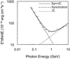 |
Fig. 1. Time-averaged spectral energy distributions (SED) of the Crab Nebula. The solid line and the binned spectrum represent the total Syn+IC emission, while the dashed and dotted lines represent the synchrotron and IC components respectively. |
3.2. Long-term light curve
In order to explore the time-variability of the synchrotron flux, we generated a light curve for the 60 MeV–600 MeV band. In this energy range, we estimate that the IC component only accounts for <8% of the integrated average flux. It is therefore justified to use a single PL as the model of the total Syn+IC emission for energies between 60 MeV and 600 MeV. Prior to temporal analyses, we performed an analysis for this energy band with the complete ten-year data set. The flux normalization of the isotropic diffuse model is found to be ≈1.13 (scaled to the full phase), and the PL spectral index for energy-dependent scaling of the Galactic diffuse model is found to be ≈0.018. Since these two parameters are not expected to noticeably change within ten years, in analyses for individual temporal segments, we fix them at the ten-year averages, while the prefactor of the Galactic diffuse model is still left free.
For the binning of the light curve we choose a time interval of five days which strikes a compromise between time-resolution and statistical uncertainties. The average photon detection rate from the Crab Nebula during the off-pulse interval chosen here is approximately 100 photons per day. In general, the statistical uncertainties of fluxes are conspicuously greater than the photon shot-noise, reflecting a small signal-to-noise ratio. For those time intervals with insufficient photon statistics (≲4 photons per day), we also place upper limits of a 95% confidence level on the nebular flux. The resulting light curve is shown in Fig. 2.
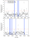 |
Fig. 2. Long-term light curve of the Crab Nebula (the total Syn+IC emission) for the 60 MeV–600 MeV band. The size of each bin is five days. The flux measurements of all bins are plotted as black circles with statistical uncertainties, while the upper limits of a 95% confidence level (only for the bins with insufficient photon statistics) are plotted as brown triangles. The black horizontal line indicates the intermediate-state average flux, while the red and blue lines respectively indicate the thresholds of the “high” and “low” states we define (see the text for detail). Blue vertical bands indicate continuous (≥15 d) “dip” features which are reported in Table 3. |
The analysis confirms the finding of previous studies that the Crab Nebula experiences a series of flares, including those reported by Buehler et al. (2012), Mayer et al. (2013), Striani et al. (2013), ATELs #8519 (Jan.-2016, around MJD 57400) and #9586 (Oct-2016, around MJD 57700). The light curve is however not well-characterized by a constant flux state superimposed by flaring activity with a small duty-cycle, resembling flicker noise. For the first time, we find that the flux occasionally drops well-below the average flux value.
This impression is confirmed when investigating the light curve in the frequency domain. The periodogram (Fig. 3) is determined via a discrete Fourier-transformation (DFT) of the real-valued light curve normalized to the average flux. The power-spectral density (PSD) is calculated from the complex valued coefficients of the DFT. The resulting PSD is characterized by a smooth PL such that PSD(f) = (0.18 ± 0.08)×(f/d−1)−0.73 ± 0.12.
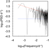 |
Fig. 3. Periodogram obtained from the long-term light curve of the Crab Nebula. The PSD is normalized to fractional variance per frequency unit. The red-solid curves in the periodogram respectively indicate the best-fit PL (whose index is 0.73 ± 0.12). The blue-dotted line indicates the white-noise PSD of a control light curve. |
The histogram of the flux measurements (Fig. 4) can be described by the superposition of two log-normal distributions (see Table 2 for the best-fit paramaters). The component A represents the extrapolated IC flux fluctuating below and around the detection threshold, with a relative normalization left free to vary in a Poissonian log-likelihood fit of the histogram. The component B characterises the variable synchrotron emission. This model is preferred over a single log-normal distribution by ∼13σ, indicating the presence of at least two different flux states. Based upon this two-component model, we set the threshold of the “low” state at 4.8 × 10⁻⁷ cm−2 s−1, so that the extrapolated tail of the component B below this threshold predicts only less than one-fourth of the observed low-state bins to be contaminated by the component B. The threshold of the “high” state is set at 5.7 × 10⁻⁶ cm−2 s−1 so that only the top 23 bins are included in the high state. In Sect. 3.5, by using simulated light curves, we confirm that a two-component model is necessary and sufficient for reproducing the continuous low-flux episodes observed (Fig. 5).
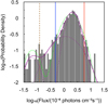 |
Fig. 4. Probability density function (PDF) obtained from the long-term light curve of the Crab Nebula. The histogram is normalised in a way such that the integration of the probability density over the log10(Flux) is 1. The double and triple log-normal models fit to the PDF are overlaid as green-dashed and purple-solid curves respectively. Their lowest-flux components model the shot-noise limited distribution of the extrapolated IC flux. The three components of the triple log-normal model are overlaid as purple-dotted curves. The blue and red vertical lines indicate the threshold of the “low” and “high” states respectively. The brown-dashed vertical line indicates the flux sensitivity corresponding to a detection significance of ∼3σ and a photon count of ∼20 in a five-day interval. |
PDF models fit to the histogram of the flux measurements.
After introducing a third log-normal component, the fitting is further improved by >6σ. The component X represents the extrapolated IC flux and it accounts for the bottom (3.3 ± 1.0)% of measurements. This corresponds to an expected 23 ± 7 out of the 68 observed low-state bins. The strongly variable component Y spans from the low flux state to the highest flux state. The component Z is mostly confined within intermediate flux states. In Sect. 3.6, we infer the relative contributions of the synchrotron nebula and IC nebula during the low state, based on spectral analyses.
We proceeded to perform an analysis with 60–600 MeV data excluding the high- and low-state bins we defined. In this way, the intermediate-state average flux is determined to be (2.61 ± 0.02stat ± 0.20sys)×10−6 cm−2 s−1, where the systematic uncertainty is determined by altering the prefactor of the Galactic diffuse model by ±10%. The statistical uncertainty in a five-day interval is generally more than a double of this systematic uncertainty. The low-state threshold we set is 18.4% of this intermediate-state average flux.
3.3. Systematic effects on the variability
The instrument, its calibration, and data analysis contribute various systematic effects that may lead to variability in excess of the limiting photon shot-noise. Similar to the approach presented by Ackermann et al. (2012), we use a data-driven method to investigate systematic effects and the stability of the light curve. Fortunately, we can use the Crab pulsar itself to establish an estimate of the instrumental variability.
We selected data collected during the phase around the highest pulse peak (0–0.02, and 0.97–1; recall that the phase convention in Buehler et al. 2012 is adopted). Then, from the total Crab flux of each bin, we subtract the nebular flux which is measured at the same bin and scaled to match the phase interval covering 5% of the total phase. The resulting light curve for the pulsar emission is based on a photon count statistics that matches the off-pulse light curve, making it suitable to be used as a control light curve.
This control light curve displays a fractional root-mean-square (RMS) variability of 14% with a PSD that is close to white noise. The resulting PSD can be readily compared with the one measured from the off-pulse emission (see Fig. 3) with a fractional RMS variability of 76%. The control light curve shows some excess noise when compared with the expected fractional variability for shot-noise only which should be  with the number of photons expected in a five-day interval (Nphot ≈ 500). We conservatively consider the noise in the control light curve as an estimate of the instrumental and photon shot noise present in the data.
The fractional RMS variability of 76% displayed in the off-pulse light curve has a significant portion accounted for by flaring bins. Even if we exclude all bins which are above the intermediate-state average, the fractional RMS variability still remains at a high value of 50%. This is a strong indication that the flux variations in the nebular light curve exceed the combined systematic and shot noise estimated from the control light curve at all frequencies (see also Fig. 3).
A limitation of the control light curve is that the 60 MeV–600 MeV spectrum of the Crab pulsar is harder than that of the nebula (Buehler et al. 2012). Any energy-dependent systematic uncertainties of Fermi LAT would, therefore, have different impacts on the nebular and pulsar light curves. As an additional check, we compute the exposure within 1° from the Crab for each five-day bin of the light curve, assuming a photon index of 3.3. Based upon this study, we have no evidence that the variability is related to fluctuations in the exposure.
Transient effects due to the relative position of the Sun or the Moon to the Crab Nebula could affect the light curve. An excess of the solar or lunar γ-ray emission could lead to an apparent deficit in the computed Crab flux. After checking the history of the Sun’s position, we do not see a causality between the observed “dip” features and solar encounters or approaches. The lunar encounters or approaches should be comparatively less of an issue, because the γ-ray emission from the Moon is much less extended (its radius of γ-ray extension is only ≲0.5°) and the Moon remains closer than seven degrees to the Crab Nebula for only <1 day (shorter than one-fifth of the bin size) in every sidereal period of 27.3 days. The periodogram of the nebular light curve reveals no distinct modulation at the lunar sidereal period or its harmonics.
Furthermore, the impact of the migration of photon energies on the nebular light curve leads to additional systematic effects. While disabling the energy dispersion correction leads to noticeable mis-measurements in the photon index, the integrated photon flux in a decade of energy range is expected to remain constant. The resulting estimated relative systematic uncertainty on the photon flux (∼1% of the flux, as evaluated in Sect. 3.1) is not important when compared to the dominating statistical uncertainty in a five-day interval.
3.4. Transitions between low-flux and intermediate states
We identified seven episodes of continuous low-flux where the 60 MeV–600 MeV Syn+IC flux remains as low as 18.4% of the intermediate-state average for at least half a month. We applied the Bayesian block algorithm (Scargle et al. 2013) on the seven analysis windows covering these episodes (Fig. 5) to identify different flux states. In turn, we quantified the transitional timescales between them by fitting composite functions to individual five-day bins in segments of the light curve.
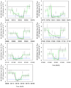 |
Fig. 5. Seven analysis windows covering continuous episodes of low-flux which are tabulated in Table 3. The uniform distribution fit to the bins of each Bayesian block (solid line) and its 1σ uncertainty (dashed line) are indicated in green. The function fit to each segment of the light curve, as well as its two exponential terms, is plotted as black curves (see the text for detail). The black and blue horizontal lines respectively indicate the intermediate-state average flux and the threshold of the “low” state we define. |
We report the time range covered by the lowest one or two successive blocks of each window as a low-flux episode. The fit range we chose for each window includes the low-flux episode as well as its preceding and following blocks. The function we fit starts and ends with two constant fluxes which are respectively equal to the local averages within the preceding and following blocks of a low-flux episode. The free parameters of the fit include the starting and stopping times of the low-flux episode where the flux varies as a sum of an exponential decay term and an exponential growth term. The predicted flux must be continuous in the whole fit range. There are in total four free parameters in the fit: in addition to the starting and stopping times, we estimate the halving time of the decay term as well as the doubling time of the growth term.
The best segmentations with a false positive rate of 0.07, as well as the functions fit to segments of the light curve, are overlaid in Fig. 5. The information about the seven episodes and the timescales of transitions are tabulated in Table 3. As a cross-check, we repeat the fits with two additional free parameters: the constant flux before decay and that after growth. We obtain consistent results. The fit results constrain the shortest timescales of transitions between low-flux and intermediate states to be <1.9 days (95% c.l.).
Information about seven episodes of continuous low-flux.
3.5. Comparison of the observed light curve to simulated light curves
The nebular emission is characterized by a red-noise PSD, dominating above instrumental noise at all frequencies sampled. In the time-domain, we have identified episodes where the flux of the nebula drops well below the average and remains low for several weeks. In order to clarify to what extent these kind of episodes occur randomly, we simulate 106 light curves following the recipe of Emmanoulopoulos et al. (2013) which has been implemented in the “DELightcurveSimulation” package (Connolly 2015). The method extends on the original approach (Tam & Yang 2012), where a method to simulate light curves with Gaussian distributed flux states and a power-law PSD is introduced. In the method used here, an arbitrarily shaped probability density function (PDF) for the flux state can be used.
The bulk of observed flux states follows a log-normal distribution. However, a noticeable deviation at lower flux states is apparent (see Fig. 4). We simulated, therefore, a log-normal PDF (with the same mean and standard deviation as the component B in Table 2) in combination with the power-law PSD (Fig. 3). In absence of a low state, we can use the simulated light curves to estimate the probability of appearance of similar episodes of low-flux as observed in the data.
We applied the Bayesian block algorithm (Scargle et al. 2013) on our observed light curve and each simulated light curve, with a false positive rate of 0.07. Then, we search for the continuous “dip” feature, which is defined as a block or a set of successive blocks fulfilling two conditions (mimicking the phenomena shown in Fig. 5): (a) the total length is at least three bins (15 days), and (b) the local mean (error-weighted) of each included block is below 4.8 × 10⁻⁷ cm−2 s−1 (the blue line in Figs. 2 and 5). Such a dip feature appears in our observed light curve for a total of seven times.
Among the simulated light curves based on the log-normal PDF, only a fraction of 5.4 × 10⁻⁵ have at least seven dips. In other words, the expected number of dips in a simulated light curve is less than that in our observed light curve at a >3.8σ level.
In order to verify that a PDF with a second, low-flux component is a closer match to the observed features in the light curve, we simulate again 106 light curves using a double log-normal distribution (Table 2) in combination with the same PSD. For this PDF, the average number of dips in a simulated light curve is 6.0 ± 1.9, which is consistent with our observations.
Repeating two chains of simulations with a more complex PSD (curved and with a constant additive term), we obtain very similar results, verifying that the exact shape of the model for the PSD is not of importance. While a double log-normal PDF is sufficient for a simulation to reproduce the seven continuous dip features we observe, we recall that the whole histogram of flux measurements suggests a more complicated distribution of flux states (see Fig. 4 and Table 2).
3.6. Spectra in different flux states
The result of the temporal analysis suggests the existence of a low-flux state (see Sects. 3.2 and 3.5). In order to investigate the spectral changes of the nebula during the defined “high” and “low” states respectively, we sort the 702 bins of the light curve according to the best-fit photon flux. The thresholds of these two flux states have been shown in Figs. 2 and 4. We group the top 23 bins above the red line into the high flux state data. For the low state, we select the lowest 68 bins below the blue line. Their accumulated TS is sufficient for us to create a binned spectrum with well-constrained uncertainties. We repeat the chain of spectral fittings described in Sect. 3.1 for the high and low states. The results are plotted in red and blue, respectively, in Fig. 6. The fit parameters are tabulated in Table 4.
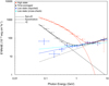 |
Fig. 6. Spectral energy distributions (SED) of the Crab Nebula for different flux states. The IC component (the dotted line) is determined with the time-averaged spectrum (in black). The spectra of the high and low states (in red and blue respectively) are defined based on the 60 MeV–600 MeV light curve of the Crab Nebula (Fig. 2). The solid lines and the binned spectra represent the total Syn+IC emission, while the dashed lines represent the synchrotron component. For the low state (solid blue line), the combined Syn+IC spectrum is plotted as a single PL component. The solid cyan line is an alternative low-state spectrum for cross-checking (see the text for detail). |
60 MeV–10 GeV spectral properties of the Crab Nebula measured in different flux states.
In both states, the binned spectra indicate that the differential flux at any energy between 1.9 GeV and 10 GeV remains consistent with the ten-year average, within the tolerance of 1.5σ uncertainties. Therefore, we fix the parameters of the IC component at the values determined with the whole ten-year data set.
During the high state, the PL index of the synchrotron component is harder than that of the ten-year average spectrum by ∼24σ, and PLEC is preferred over PL by ∼10.7σ, confirming previous results on the flaring state of the Crab Nebula (Buehler et al. 2012; Mayer et al. 2013). The differential low-state spectrum (shown in Fig. 6 in blue) differs from the average spectrum too. During the low state, the energy spectrum of the synchrotron component cannot be well described by PL or PLEC with physically reasonable parameters, so we just report the synchrotron flux computed directly from the binned spectrum, which is (15 ± 5)% of the ten-year average.
On the other hand, the entire Syn+IC spectrum during the low state can be fit by a single PL component, despite a potential excess in the lowest energy bin (∼2.5σ). Such an outlying bin is measured with 60–129 MeV data, which is limited by particularly poor spatial and spectral resolutions of LAT as well as the severe inaccuracy on the part of diffuse models. This PL has a hard index (1.65 ± 0.05) and a low integral flux which are quite comparable to those of the ten-year average IC component. The γ-ray luminosity of the IC component is 77% of the low-state luminosity of the whole Crab Nebula computed from this model.
We note that 22 out of the 68 low-state bins have their preceding and following bins both ≥44% of the intermediate-state average. They can be considered “isolated” (i.e., not in pairs or clusters). On average, a mock light curve simulated with the log-normal PDF and the power-law PSD (reported in Sect. 3.5) has 16.2 ± 4.0 low-state bins where 2.0 ± 1.7 of them are isolated in the same way. We recall that the combined systematic and shot noise has a fractional RMS variability of ∼14% (as evaluated in Sect. 3.3). Also, immediately before and after a low-flux bin, the Crab Nebula is probably in a similar physical state for a while. These entail a statement that some isolated low-state bins in the observed nebular light curve could be occasional chance events. Therefore, the numerous discontinuities in our selection of low-state bins could have introduced non-negligible systematic bias in measuring the low-state spectral properties.
With regards to this issue, we reconstructed an alternative low-state spectrum as a cross-check. In order to investigate the spectrum for clusters of low-flux bins, we grouped a total of 41 bins of the seven continuous low-flux episodes (Table 3) into this alternative low-state, and the obtained result is overlaid in Fig. 6 as well. It turns out that the two low-state spectra have very similar integrated fluxes and photon indices.
4. Summary and conclusion
4.1. Summary of main results
4.1.1. Variability and low-flux state of the synchrotron nebula
The long-term light curve of the gamma-ray emission from the Crab Nebula in the energy range between 60 MeV and 600 MeV has been extracted from ten years of observation with the Fermi LAT instrument. On average, >92% of the integrated flux is accounted for by synchrotron radiation. The light curve shows pronounced variability, with a relative standard deviation equal to 76%. As demonstrated with a control light curve from a phase-gated part of the pulsar emission, we estimate that less than 2% of the measured variability could be related to instrumental or systematic effects. The periodogram follows a PL with an index of 0.73 ± 0.12, indicating the presence of flicker-noise in the entire frequency range covered by the observations. In the observed light curve, we identify at least seven episodes during which the source flux drops below 18.4% of the intermediate-state average. Using Bayesian blocks, we characterize these episodes to last between five and 35 days. We used simulated light curves to estimate the probability of chance appearance of these episodes for a variable source characterized by a single log-normal distribution of flux states and a PSD with the same spectral shape as found for the observed light curve. We infer a probability of ∼5.4 × 10⁻⁵ of having the number of continuous (≥15 d) low-flux episodes detected in a simulation greater than or equal to that in our observed light curve. A superposition of two log-normal distributions is sufficient for a simulation to reproduce the seven continuous dip features we observe. On the other hand, a PDF model containing three log-normal components is statistically favored to describe the entire histogram of flux measurements.
Energy spectrum during different flux states. The energy spectra have been extracted in three flux intervals respectively. The binned spectra in the energy range from 2 GeV to 10 GeV implies that the state transitions do not lead to any noticeable change in the IC component up to 10 GeV. After all, the IC component is intrinsically steady during the lifetime of the Crab Nebula, because the responsible low-energy electrons fill a large volume with a cooling timescale exceeding the age of the nebula. We confirm the general trend of a hardening and curvature of the synchrotron spectrum in the high-flux state, which is discussed in Buehler et al. (2012) and Mayer et al. (2013). For the first time, we reconstruct the energy spectrum in the newly found low-flux state. The energy spectrum in the low-flux state and at energies below 2 GeV is roughly consistent with an extrapolation of the IC component of the nebula emission towards lower energies.
Notably, the fitting for the IC component is dominated by the >2 GeV data, leading to a large uncertainty in its extrapolated flux below 600 MeV. Also, we found an energy-dependent spatial extension of the IC nebula, where the size shrinks as the photon energy increases (Yeung & Horns 2019). The extrapolated extension size (the 68% containment radius) at 100 MeV is as large as 0.1°. However, we model the IC component as a point source in this work, which only accounts for a core part of the IC nebula. Therefore, the extrapolated IC flux could have been underestimated while the measured low-state spectrum provides an indication to the actual IC nebula emission.
We therefore conclude from the characterization of the variability and the spectral analysis that the synchrotron nebular emission between 60 MeV and 600 MeV drops well below the average flux on time-scales of several days and remains in a low state for several weeks. During these episodes of low-state emission, the predomination of the nebular energy spectrum by the IC emission demonstrates that the high-energy part of the synchrotron nebula is dramatically depressed on a short time-scale.
We consider in the following a possible interpretation of a compact emission region which satisfies the requirement that the emission region is causally connected within the variability time-scale found during the transition phase of less than two days. This compact region would be the origin of the bulk of the observed emission such that it would explain simultaneously the rapid dimming of the entire emission, as well as the low-state spectrum which is apparently dominated by the constant flux of the IC nebula. Possible alternative explanations based upon variability of the entire nebula need to circumvent the argument of causal connection. Here, we focus on the well-known inner knot observed near the pulsar’s position (Hester et al. 1995) as a possible candidate.
4.2. Interpretation as synchrotron emission from the inner knot
With the shortest timescales of transitions between low-flux and intermediate states constrained to be less than two days (95% c.l.), we infer that at least 75% of the >108 eV emission of the so-called synchrotron nebula originate from a compact region with an extension limited by the light crossing time to be ctvar ≈ 4.2 mpc tvar/(5 d) which corresponds to an angular diameter (at a distance of 2.2 kpc) of  . The time-scale of variability and the inferred angular extension of
  is consistent with the finding of Rudy et al. (2015), where the tangential FWHM of the knot was observed to be 0.3″ − 0.35″. The result of our analysis of the variability therefore strengthens the interpretation that the high-energy part of the synchrotron emission is produced in the inner knot of the Crab Nebula as put forward by Komissarov & Lyutikov (2011).
The inner knot has also been found to show variability in the optical and X-ray band (Rudy et al. 2015) with correlations of the knot’s morphology and position with its gamma-ray flux that are similar to the expectations of models of the termination shock (Lyutikov et al. 2016). Further multi-wavelength observations of the inner knot during a phase of the 60 MeV–600 MeV low-state would be essential to confirm the proposed scenario.
Acknowledgments
PKHY acknowledges the support of the DFG under the research grant HO 3305/4-1. We greatly appreciate M. Kerr for providing the ephemeris of the Crab pulsar for phased analysis. PKHY thanks H.-F. Yu for useful discussions. We thank the two anonymous referees for very useful comments which helped to improve the manuscript.
References
- Abdo, A. A., Ackermann, M., Ajello, M., et al. 2011, Science, 331, 739 [NASA ADS] [CrossRef] [PubMed] [Google Scholar]
- Ackermann, M., Ajello, M., Albert, A., et al. 2012, ApJS, 203, 4 [NASA ADS] [CrossRef] [Google Scholar]
- Aharonian, F., Akhperjanian, A., Beilicke, M., et al. 2004, ApJ, 614, 897 [NASA ADS] [CrossRef] [Google Scholar]
- Atoyan, A. M., & Aharonian, F. A. 1996, MNRAS, 278, 525 [NASA ADS] [Google Scholar]
- Buehler, R., Scargle, J. D., Blandford, R. D., et al. 2012, ApJ, 749, 26 [NASA ADS] [CrossRef] [Google Scholar]
- Bühler, R., & Blandford, R. 2014, Rep. Prog. Phys., 77, 066901 [NASA ADS] [CrossRef] [PubMed] [Google Scholar]
- Connolly, S. D. 2015, ArXiv e-prints [arXiv:1503.06676] [Google Scholar]
- de Jager, O. C., & Harding, A. K. 1992, ApJ, 396, 161 [NASA ADS] [CrossRef] [Google Scholar]
- Dubner, G., Castelletti, G., Kargaltsev, O., et al. 2017, ApJ, 840, 82 [CrossRef] [Google Scholar]
- Emmanoulopoulos, D., McHardy, I. M., & Papadakis, I. E. 2013, MNRAS, 433, 907 [NASA ADS] [CrossRef] [Google Scholar]
- Fraschetti, F., & Pohl, M. 2017, MNRAS, 471, 4856 [NASA ADS] [CrossRef] [Google Scholar]
- Gunn, J. E., & Ostriker, J. P. 1971, ApJ, 165, 523 [NASA ADS] [CrossRef] [Google Scholar]
- Hester, J. J. 2008, Ann. Rev. Astron. Astrophys., 46, 127 [NASA ADS] [CrossRef] [Google Scholar]
- Hester, J. J., Scowen, P. A., Sankrit, R., et al. 1995, ApJ, 448, 240 [NASA ADS] [CrossRef] [Google Scholar]
- Hillas, A. M., Akerlof, C. W., Biller, S. D., et al. 1998, ApJ, 503, 744 [NASA ADS] [CrossRef] [Google Scholar]
- Komissarov, S. S., & Lyutikov, M. 2011, MNRAS, 414, 2017 [NASA ADS] [CrossRef] [Google Scholar]
- Kuiper, L., Hermsen, W., Cusumano, G., et al. 2001, A&A, 378, 918 [NASA ADS] [CrossRef] [EDP Sciences] [Google Scholar]
- Ling, J. C., & Wheaton, W. A. 2003, ApJ, 598, 334 [NASA ADS] [CrossRef] [Google Scholar]
- Lobanov, A. P., Horns, D., & Muxlow, T. W. B. 2011, A&A, 533, A10 [NASA ADS] [CrossRef] [EDP Sciences] [Google Scholar]
- Lyutikov, M., Komissarov, S., & Porth, O. 2016, MNRAS, 456, 286 [CrossRef] [Google Scholar]
- Martín, J., Torres, D. F., & Rea, N. 2012, MNRAS, 427, 415 [NASA ADS] [CrossRef] [Google Scholar]
- Meyer, M., Horns, D., & Zechlin, H.-S. 2010, A&A, 523, A2 [NASA ADS] [CrossRef] [EDP Sciences] [Google Scholar]
- Mayer, M., Buehler, R., Hays, E., et al. 2013, ApJ, 775, L37 [NASA ADS] [CrossRef] [Google Scholar]
- Rees, M. 1971, J. Nat. Phys. Sci., 230, 55 [CrossRef] [Google Scholar]
- Rudy, A., Horns, D., DeLuca, A., et al. 2015, ApJ, 811, 24 [NASA ADS] [CrossRef] [Google Scholar]
- Scargle, J. D., Norris, J. P., Jackson, B., & Chiang, J. 2013, ApJ, 764, 167 [NASA ADS] [CrossRef] [Google Scholar]
- Spitkovsky, A., & Arons, J. 2004, ApJ, 603, 669 [NASA ADS] [CrossRef] [Google Scholar]
- Striani, E., Tavani, M., Vittorini, V., et al. 2013, ApJ, 765, 52 [NASA ADS] [CrossRef] [Google Scholar]
- Tam, H., & Yang, Q. 2012, Phys. Lett. B, 716, 435 [CrossRef] [Google Scholar]
- Tavani, M., Bulgarelli, A., Vittorini, V., et al. 2011, Science, 331, 736 [NASA ADS] [CrossRef] [PubMed] [Google Scholar]
- The Fermi-LAT Collaboration 2019, ArXiv e-prints [arXiv:1902.10045] [Google Scholar]
- Trimble, V. 1968, ApJ, 73, 535 [NASA ADS] [CrossRef] [Google Scholar]
- Volpi, D., Del Zanna, L., Amato, E., & Bucciantini, N. 2008, A&A, 485, 337 [NASA ADS] [CrossRef] [EDP Sciences] [Google Scholar]
- Wilson-Hodge, C. A., Cherry, M. L., Case, G. L., et al. 2011, ApJ, 727, L40 [NASA ADS] [CrossRef] [Google Scholar]
- Yeung, P. K. H., & Horns, D. 2019, ApJ, 875, 123 [CrossRef] [Google Scholar]
All Tables
Time-averaged spectral properties of the Crab Nebula measured from 60 MeV to 10 GeV.
60 MeV–10 GeV spectral properties of the Crab Nebula measured in different flux states.
All Figures
|
Fig. 1. Time-averaged spectral energy distributions (SED) of the Crab Nebula. The solid line and the binned spectrum represent the total Syn+IC emission, while the dashed and dotted lines represent the synchrotron and IC components respectively. |
| In the text | |
|
Fig. 2. Long-term light curve of the Crab Nebula (the total Syn+IC emission) for the 60 MeV–600 MeV band. The size of each bin is five days. The flux measurements of all bins are plotted as black circles with statistical uncertainties, while the upper limits of a 95% confidence level (only for the bins with insufficient photon statistics) are plotted as brown triangles. The black horizontal line indicates the intermediate-state average flux, while the red and blue lines respectively indicate the thresholds of the “high” and “low” states we define (see the text for detail). Blue vertical bands indicate continuous (≥15 d) “dip” features which are reported in Table 3. |
| In the text | |
|
Fig. 3. Periodogram obtained from the long-term light curve of the Crab Nebula. The PSD is normalized to fractional variance per frequency unit. The red-solid curves in the periodogram respectively indicate the best-fit PL (whose index is 0.73 ± 0.12). The blue-dotted line indicates the white-noise PSD of a control light curve. |
| In the text | |
|
Fig. 4. Probability density function (PDF) obtained from the long-term light curve of the Crab Nebula. The histogram is normalised in a way such that the integration of the probability density over the log10(Flux) is 1. The double and triple log-normal models fit to the PDF are overlaid as green-dashed and purple-solid curves respectively. Their lowest-flux components model the shot-noise limited distribution of the extrapolated IC flux. The three components of the triple log-normal model are overlaid as purple-dotted curves. The blue and red vertical lines indicate the threshold of the “low” and “high” states respectively. The brown-dashed vertical line indicates the flux sensitivity corresponding to a detection significance of ∼3σ and a photon count of ∼20 in a five-day interval. |
| In the text | |
|
Fig. 5. Seven analysis windows covering continuous episodes of low-flux which are tabulated in Table 3. The uniform distribution fit to the bins of each Bayesian block (solid line) and its 1σ uncertainty (dashed line) are indicated in green. The function fit to each segment of the light curve, as well as its two exponential terms, is plotted as black curves (see the text for detail). The black and blue horizontal lines respectively indicate the intermediate-state average flux and the threshold of the “low” state we define. |
| In the text | |
|
Fig. 6. Spectral energy distributions (SED) of the Crab Nebula for different flux states. The IC component (the dotted line) is determined with the time-averaged spectrum (in black). The spectra of the high and low states (in red and blue respectively) are defined based on the 60 MeV–600 MeV light curve of the Crab Nebula (Fig. 2). The solid lines and the binned spectra represent the total Syn+IC emission, while the dashed lines represent the synchrotron component. For the low state (solid blue line), the combined Syn+IC spectrum is plotted as a single PL component. The solid cyan line is an alternative low-state spectrum for cross-checking (see the text for detail). |
| In the text | |
Current usage metrics show cumulative count of Article Views (full-text article views including HTML views, PDF and ePub downloads, according to the available data) and Abstracts Views on Vision4Press platform.
Data correspond to usage on the plateform after 2015. The current usage metrics is available 48-96 hours after online publication and is updated daily on week days.
Initial download of the metrics may take a while.