| Issue |
A&A
Volume 638, June 2020
|
|
|---|---|---|
| Article Number | A11 | |
| Number of page(s) | 23 | |
| Section | Planets and planetary systems | |
| DOI | https://doi.org/10.1051/0004-6361/201936380 | |
| Published online | 03 June 2020 | |
Physical parameters of selected Gaia mass asteroids
1
Astronomical Observatory Institute, Faculty of Physics, Adam Mickiewicz University,
Słoneczna 36,
Poznań,
Poland
e-mail: This email address is being protected from spambots. You need JavaScript enabled to view it.
2
Max-Planck-Institut für extraterrestrische Physik (MPE),
Giessenbachstrasse 1,
85748
Garching,
Germany
3
Konkoly Observatory, Research Centre for Astronomy and Earth Sciences, Hungarian Academy of Sciences,
1121 Budapest,
Konkoly Thege Miklós
út 15-17,
Hungary
4
Instituto de Astrofísica de Andalucía (CSIC),
Glorieta de la Astronomía s/n,
18008
Granada,
Spain
5
MTA CSFK Lendület Near-Field Cosmology Research Group,
Budapest,
Hungary
6
Astronomy Department, Eötvös Loránd University,
Pázmány P. s. 1/A,
H-1171
Budapest,
Hungary
7
Observatoire des Hauts Patys,
84410
Bedoin,
France
8
Asociación Astronómica Astro Henares,
Centro de Recursos Asociativos El Cerro C/ Manuel Azaña,
28823
Coslada,
Spain
9
B92 Observatoire de Chinon,
Chinon,
France
10
Oukaimeden Observatory, High Energy Physics and Astrophysics Laboratory, Cadi Ayyad University,
Marrakech,
Morocco
11
Geneva Observatory,
1290
Sauverny,
Switzerland
12
Observatoire des Engarouines,
1606 chemin de Rigoy,
84570
Malemort-du-Comtat,
France
13
B74, Avinguda de Catalunya 34,
25354
Santa Maria de Montmagastrell (Tàrrega),
Spain
14
I39, Cruz del Sur Observatory,
San Justo city,
Buenos Aires,
Argentina
15
Space Sciences, Technologies and Astrophysics Research Institute, Université de Liège,
Allée du 6 Août 17,
4000
Liège,
Belgium
16
Instituto de Astrofísica de Canarias,
C/ Vía Lactea s/n,
38205
La Laguna,
Tenerife,
Spain
17
Gran Telescopio Canarias (GRANTECAN),
Cuesta de San José s/n,
38712,
Breña Baja,
La Palma,
Spain
18
School of Physical Sciences, The Open University,
MK7 6AA,
UK
19
Observatoire des Terres Blanches,
04110
Reillanne,
France
20
I64,
SL6 1XE
Maidenhead,
UK
21
Anunaki Observatory, Calle de los Llanos,
28410
Manzanares el Real,
Spain
22
The IEA, University of Reading,
Philip Lyle Building, Whiteknights Campus,
Reading,
RG6 6BX,
UK
23
Rue des Ecoles 2,
34920
Le Cres,
France
24
Observatoire de Blauvac,
293 chemin de St Guillaume,
84570
Blauvac,
France
25
University of Ljubljana, Faculty of Mathematics and Physics Astronomical Observatory,
Jadranska 19
1000
Ljubljana,
Slovenia
26
Departamento de Física, Ingeniería de Sistemas y Teoría de la Señal, Universidad de Alicante,
03080
Alicante,
Spain
27
Institut de Ciéncies del Cosmos, Universitat de Barcelona (IEEC-UB),
Martí i Franqués 1,
08028
Barcelona,
Spain
Received:
25
July
2019
Accepted:
20
December
2019
Abstract
Context. Thanks to the Gaia mission, it will be possible to determine the masses of approximately hundreds of large main belt asteroids with very good precision. We currently have diameter estimates for all of them that can be used to compute their volume and hence their density. However, some of those diameters are still based on simple thermal models, which can occasionally lead to volume uncertainties as high as 20–30%.
Aims. The aim of this paper is to determine the 3D shape models and compute the volumes for 13 main belt asteroids that were selected from those targets for which Gaia will provide the mass with an accuracy of better than 10%.
Methods. We used the genetic Shaping Asteroids with Genetic Evolution (SAGE) algorithm to fit disk-integrated, dense photometric lightcurves and obtain detailed asteroid shape models. These models were scaled by fitting them to available stellar occultation and/or thermal infrared observations.
Results. We determine the spin and shape models for 13 main belt asteroids using the SAGE algorithm. Occultation fitting enables us to confirm main shape features and the spin state, while thermophysical modeling leads to more precise diameters as well as estimates of thermal inertia values.
Conclusions. We calculated the volume of our sample of main-belt asteroids for which the Gaia satellite will provide precise mass determinations. From our volumes, it will then be possible to more accurately compute the bulk density, which is a fundamental physical property needed to understand the formation and evolution processes of small Solar System bodies.
Key words: minor planets, asteroids: general / techniques: photometric / radiation mechanisms: thermal
© ESO 2020
1 Introduction
Thanks to the development of asteroid modeling methods (Kaasalainen et al. 2002; Viikinkoski et al. 2015; Bartczak & Dudziński 2018), the last two decades have allowed for a better understanding of the nature of asteroids. Knowledge about their basic physical properties helps us to not only understand particular objects, but also the asteroid population as a whole. Nongravitational effects with a proven direct impact on asteroid evolution, such as the Yarkovsky-O’Keefe-Radzievskii-Paddack (YORP) and Yarkovsky effects, could not be understood without a precise knowledge about the spin state of asteroids. For instance, the sign of the orbital drift induced by the Yarkovsky effect depends on the target’s sense of rotation (Rubincam 2001). Also, spin clusters have been observed among members of asteroid families (Slivan 2002) that are best explained as an outcome of the YORP effect (Vokrouhlický et al. 2003, 2015).
Precise determinations of the spin and shape of asteroids will be of the utmost significance for improving the dynamical modeling of the Solar System and also for our knowledge of the physics of asteroids. From a physical point of view, the mass and size of an asteroid yield its bulk density, which accounts for the amount of matter that makes up the body and the space occupied by its pores and fractures. For a precise density determination, we need a model of the body, whichrefers to its 3D shape and spin state. These models are commonly obtained from relative photometric measurements. In consequence, an estimation of the body size is required in order to scale the model. The main techniques used for size determination (for a review, see e.g., Ďurech et al. 2015) are stellar occultations, radiometric techniques, or adaptive optics (AO) imaging, as well as the in situ exploration of spacecrafts for a dozen of visited asteroids.
The disk-integrated lightcurves obtained from different geometries (phase and aspect angles) can give us a lot of information about the fundamental parameters, such as rotation period, spin axis orientation, and shape. However, the shape obtained from lightcurve inversion methods is usually scale-free. Thus, we need to use other methods to express them in kilometers and calculate the volumes. The determination of asteroid masses is also not straightforward, but it is expected that Gaia, thanks to its precise astrometric measurements, will be able to provide masses for more than a hundred asteroids. This is possible for objects that undergo gravitational perturbations during close approaches with other minor bodies (Mouret et al. 2007).
There are already a few precise sizes that are available based on quality spin and shape models of Gaia mass targets, including convex inversion and All-Data Asteroid Modeling (ADAM) shapes (some based on Adaptive Optics, Vernazza et al. 2019). However, there are still many with only Near Earth Asteroid Thermal Model (NEATM) diameters. In this paper, we use the SAGE (Shaping Asteroids with Genetic Evolution) algorithm (Bartczak & Dudziński 2018) and combine it with thermo-physical models (TPM) and/or occultations to determine the shape, spin, and absolute scale of a list of Gaia targets in order to calculate their densities. As a result, here, we present the spin solutions and 3D shape models of 13 large main belts asteroids for which they are expected to have mass measurements from the Gaia mission with a precision of better than 10%. For some objects, we compare our results with already existing models to test the reliability of our methods. Thanks to the increased photometric datasets produced by our project, previously existing solutions have been improved for the asteroids that were selected, and for two targets for which we determine the physical properties for the first time. We provide the scale and volume for all the bodies that are studied with realistic error bars. These volumes combined with the masses from Gaia astrometry will enable precise bulk density determinations and further mineralogical studies. The selected targets are mostly asteroids with diameters larger than 100 km, which are considered to be remnants of planetesimals (Morbidelli et al. 2009). These large asteroids are assumed to only have small macroporosity, thus their bulk densities can be used for comparison purposes with spectra.
The paper is organized as follows. In Sect. 2 we present our observing campaign, give a brief description of the spin and shape modeling technique, including the quality assessment of the solution, and describe the fitting to the occultation chords and the thermophysical modeling. In Sect. 3 we show the results of our study of 13 main belt asteroids, and in Sect. 4 we summarize our findings. Appendix A presents the results of TPM modeling, while Appendix B contains fitting the SAGE shape models to stellar occultations.
2 Methodology
2.1 Observing campaign
In order to construct precise spin and shape models for asteroids, we used dense photometric disk-integrated observations. Reliable asteroid models require lightcurves from a few apparitions, that are well distributed along the ecliptic longitude. The available photometric datasets for selected Gaia mass targets are complemented by an observing campaign that provided data from unique geometries, which improved the existing models by probing previously unseen parts of the surface. Using the Super-WASP (Wide Angle Search for Planets) asteroid archive (Grice et al. 2017) was also very helpful, as it provided data from unique observing geometries. Moreover, in many cases new data led to updates of sidereal period values. The coordination of observations was also very useful for long period objects, for which the whole rotation could not be covered from one place during one night. We gathered our new data during the observing campaign in the framework of the H2020 project called Small Bodies Near And Far (SBNAF, Müller et al. 2018). The main observing stations were located in La Sagra (IAA CSIC, Spain), Piszkéstető (Hungary), and Borowiec (Poland), and the observing campaign was additionally supported by the GaiaGOSA web service dedicated toamateur observers (Santana-Ros et al. 2016). For some objects, our data were complemented by data from the K2 mission of the Kepler space telescope (Szabó et al. 2017) and the TRAPPIST North and South telescopes (Jehin et al. 2011). Gathered photometric data went through careful analysis in order to remove any problematic issues, such as star passages, color extinction, bad pixels, or other instrumental effects. In order to exclude any unrealistic artefacts, we decided not to take into account data that were too noisy or suspect data. The most realistic spin and shape models can be reconstructed when the observations are spread evenly along the orbit; this allows one to observe all illuminated parts of the asteroid’s surface. Therefore, in this study, we particularly concentrated on the observations of objects for which we could cover our targets in previously unseen geometries, which is similar to what was done for 441 Bathilde, for which data from 2018 provided a lot of valuable information.Figure 1 shows an example of the ecliptic longitude coverage for the asteroid 441 Bathilde.
2.2 Spin and shape modeling
We used the genetic algorithm, SAGE to calculate asteroid models (Bartczak & Dudziński 2018). SAGE allowed us to reproduce spin and nonconvex asteroid shapes based exclusively on photometric lightcurves. Here, we additionally introduce the recently developed quality assessment system (Bartczak & Dudziński 2019), which gives information about the reliability of the obtained models. Theuncertainty of the SAGE spin and shape solutions was calculated by the multiple cloning of the final models and by randomly modifying the size and radial extent of their shape features. These clones were checked for their ability to simultaneously reproduce all the lightcurves within their uncertainties. By lightcurve uncertainty, we are referringto the uncertainty of each point. For the lightcurves with no uncertainty information, we adopted 0.01 mag. This way, the scale-free dimensions with the most extreme, but still possible shape feature modifications, were calculated and then translated to diameters in kilometers by fitting occultation chords. Some of the calculated models can be compared to the solutions obtained from other methods, which often use adaptive optics images, such as KOALA (Knitted Occultation, Adaptive-optics, and Lightcurve Analysis, Carry et al. 2010) and ADAM (Viikinkoski et al. 2015). Such models are stored in the DAMIT Database of Asteroid Models from Inversion Techniques (DAMIT) database1 (Ďurech et al. 2010). Here, we show the nonconvex shapes that were determined with the SAGE method. We have only used the photometricdata since they are the easiest to use and widely available data for asteroids. It should be noted, however, that some shape features, such as the depth of large craters or the height of hills, are prone to the largest uncertainty, as was shown by Bartczak & Dudziński (2019). It is also worth mentioning here that such a comparison of two methods is valuable as a test for the reliability of two independent methods and for the correctness of the existing solutions with the support of a wider set of photometric data. For a few targets from our sample, we provide more realistic, smoother shape solutions, which improve on the previously existing angular shape representations based on limited or sparse datasets. For two targets, (145) Adeona and (308) Polyxo, the spin and shape solutions were obtained here for the first time.
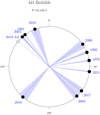 |
Fig. 1 Observer-centered ecliptic longitude of asteroid (441) Bathilde at apparitions with well covered lightcurves. |
2.3 Scaling the models by stellar occultations
The calculated spin and shape models are usually scale-free. By using two independent methods, the stellar occultation fitting and thermophysical modeling, we were able to provide an absolute scale for our shape models. The great advantage of the occultation technique is that the dimensions of the asteroid shadow seen on Earth can be treated as a real dimension of the object. Thus, if enough chords are observed, we can express the size of the object in kilometers. Moreover, with the use of multichord events, the major shape features can be recovered from the contours. To scale our shape models, we used the occultation timings stored in the Planetary Data System (PDS) database (Dunham et al. 2016). Only the records with at least three internally consistent chords were taken into account. The fitting of shape contours to events with fewer chords is burdened with uncertainties that are too large.
Three chords also do not guarantee precise size determinations because of substantial uncertainties in the timing of some events or the unfortunate spatial grouping of chords. We used the procedure implemented in Ďurech et al. (2011) to compare our shape models with available occultation chords. We fit the three parameters ξ, η (the fundamental plane here is defined the same as in Ďurech et al. 2011), and c, which was scaled in order to determine the size. The shape models’ orientations were overlayed on the measured occultation chords and scaled to minimize χ2 value. The difference with respect to the procedure described in Ďurech et al. (2011) is that we fit the projection silhouette to each occultation event separately, and we took the confidence level of the nominal solution into account as it was described in Bartczak & Dudziński (2019). We also did not optimize offsets of the occultations. Shape models fitting to stellar occultations with accompanying errors are presented in Figs. C.1–C.10. The final uncertainty in the volume comes from the effects of shape and occultation timing uncertainties and it is usually larger than in TPM since thermal data are very sensitive to the size of the body and various shape features play a lesser role there. On the other hand, precise knowledge of the sidereal period and spin axis position is of vital importance for the proper phasing of the shape models in both TPM and in occultation fitting. So, if a good fit is obtained by both methods, we consider it to be a robust confirmation for the spin parameters.
2.4 Thermophysical modeling (TPM)
The TPM implementation we used is based on Delbo & Harris (2002) and Alí-Lagoa et al. (2014). We already described our approach in Marciniak et al. (2018, 2019), which give details about the modeling of each target. So in this section, we simply provide a brief summary of the technique and approximations we make. In Appendix A, we include all the plots that are relevant to the modeling of each target and we provide some additional comments.
The TPM takes the shape model as input, and its main goal is to model the temperature on any given surface element (facet) at each epoch at which we have thermal IR (infrared) observations, so that the observed flux can be modeled. To account for heat conduction toward the subsurface, we solved the 1D heat diffusion equation for each facet and we used the Lagerrosapproximation for roughness (Lagerros 1996, 1998; Müller & Lagerros 1998; Müller 2002). We also consider thespectral emissivity to be 0.9 regardless of the wavelength (see, e.g., Delbo et al. 2015). We explored different roughness parametrizations by varying the opening angle of hemispherical craters covering 0.6 of the area of the facets (following Lagerros 1996). For each target, we estimated the Bond albedo that was used in the TPM as the average value that was obtained from the different radiometric diameters available from AKARI and/or WISE (Wright et al. 2010; Usui et al. 2011; Alí-Lagoa et al. 2018; Mainzer et al. 2016), and all available H-G, H-G12, and H-G1-G2 values from the Minor Planet Center (Oszkiewicz et al. 2011, or Veres et al. 2015).
This approach leaves us with two free parameters, the scale of the shape (interchangeably called the diameter, D), and the thermal inertia (Γ). The diameters, which were calculated as volume-equivalent diameters, and other relevant information related to the TPM analyses of our targets are provided in Table A.1. Whenever there are not enough data to provide realistic error bar estimates, we report the best-fitting diameter so that the models can be scaled and compared to the scaling given by the occultations. On the other hand, if we have multiple good-quality thermal data, with absolute calibration errors below 10%, then this typically translates to a size accuracy of around 5% as long as the shape is not too extreme and the spin vector is reasonably well established. This general rule certainly works for large main belt asteroids, that is, the Gaia mass targets. We do not consider the errors that are introduced by the pole orientation uncertainties or the shapes (see Hanuš et al. 2016 and Bartczak & Dudziński 2019); therefore, our TPM error bars are lower estimates of the true error bars. The previously mentioned general rule or expectation is based on the fact that the flux is proportional to the square of the projected area, so fitting a high-quality shape and spin model to fluxes with 10% absolute error bars should produce a ~ 5% accurate size. This is verified by the large asteroids that were used as calibrators (Müller 2002; Harris & Lagerros 2002; Müller et al. 2014).
Nonetheless, we would still argue that generally speaking, scaling 3D shapes, which were only determined via indirect means (such as pure LC inversion) by modeling thermal IR data that were only observed close to pole-on, could potentially result in a biased TPMsize if the shape has an over- or underestimated z-dimension (e.g., Bartczak & Dudziński 2019). This also happens with at least some radar models (e.g., Rozitis & Green 2014).
3 Results
The following subsections describe our results for each target, whereas Tables 1, 2, and A.1 provide the pole solutions, the results from the occultation fitting, and the results from TPM, respectively. The fit of the models to the observed lightcurves can be found for each object on the ISAM2 (Interactive Service for Asteroid Models) web-service (Marciniak et al. 2012). On ISAM, we also show the fit of available occultation records for all objects studied in this paper. For comparison purposes, a few examples are given for SAGE shape models and previously existing solutions, which are shown in Figs. 2–6, as well as for previous period determinations and pole solutions, which are given in Table A.2. For targets without previously available spin and shape models, we determined the model based on the simple lightcurve inversion method (see Kaasalainen et al. 2002), such as in Marciniak et al. (2018), and we compared the results with those from the SAGE method.
3.1 (3) Juno
We used observations from 11 apparitions to model Juno’s shape. All lightcurves display amplitude variations from 0.12 to 0.22 mag, which indicates the body has a small elongation. Juno was already investigated with the ADAM method by Viikinkoski et al. (2015), which was based on ALMA (Atacama Large Millimeter Array) and adaptive optics data in addition to lightcurves. The rotation period and spin axis position of both models, ADAM and SAGE, are in good agreement. However, the shapes look different from some perspectives. The shape contours of the SAGE model are smoother and the main features, such as polar craters, were reproduced in both methods. We compared our SAGE model with AO data and the results from ADAM modeling by Viikinkoski et al. (2015) in Fig. 2. The fit is good, but not perfect.
A rich dataset of 112 thermal infrared measurements is available for (3) Juno, including unpublished Herschel PACS data (Müller et al. 2005). The complete PACS catalog of small-body data will be added to the SBNAF infrared database once additional SBNAF articles are published. For instance, the full TPM analysis of Juno will be included in an accompanying paper that features the rest of the PACS main-belt targets (Alí-Lagoa et al., in prep.). Here, we include Juno in order to compare the scales we obtained from TPM and occultations.
TPM leads to a size of 254 ± 4 km (see Tables 2 and A.1), which is in agreement with the ADAM solution (248 km) within the error bars. The stellar occultations from the years 1979, 2000, and 2014 also fit well (see Fig. C.1 for details). The 1979 event, which had the most dense coverage (15 chords), leads to a diameter of  km.
km.
3.2 (14) Irene
For (14) Irene, we gathered the lightcurves from 14 apparitions, but from very limited viewing geometries. The lightcurve shapes were very asymmetric, changing character from bimodal to monomodal in some apparitions, which indicates large aspect angle changes caused by low spin axis inclination to the orbital plane of the body. The amplitudes varied from 0.03 to 0.16 mag. The obtained SAGE model fits very well to the lightcurves; the agreement is close to the noise level. The spin solution is presented in Table 1. The SAGE model is in very good agreement with the ADAM model, which displays the same major shape features (see Fig. 3). This agreement can be checked for all available models by generating their sky projections at the same moment on the ISAM and DAMIT3 webpages.
The only three existing occultation chords seem to point to the slightly preferred SAGE solution from two possible mirror solutions (Fig. C.2), and it led to a size of  km for the pole 1 solution. The TPM fit resulted in a compatible size of 155 km, which is in good agreement within the error bars. We note, however, that the six thermal IR data available are not substantial enough to give realistic TPM error bars (the data are fit with an artificially low minimum that was reduced to χ2 ~ 0.1), but nonetheless both of our size determinations here also agree with the size of the ADAM shape model based on the following adaptive optics imaging: 153 km ± 6 km (Viikinkoski et al. 2017).
Spin parameters of asteroid models obtained in this work, with their uncertainty values.
3.3 (20) Massalia
Data from 13 apparitions were at our disposal to model (20) Massalia, although some of them were grouped close together in ecliptic longitudes. Massalia displayed regular, bimodal lightcurve shapes with amplitudes from 0.17 to 0.27 mag. New data gathered within the SBNAF and GaiaGOSA projects significantly improved the preliminary convex solution that exists in DAMIT (Kaasalainen et al. 2002), which has a much lower pole inclination and a sidereal period of 0.002 hours shorter. If we consider the long span (60 yr) of available photometric data and the shortness of the rotation period, such a mismatch causes a large shift in rotational phase after a large number of rotations.
The two SAGE mirror solutions have a smooth shape with a top shape appearance. Their fit to the occultation record from 2012 led to two differing size solutions of  and
and  km (Fig. C.3); both are smaller and outside the combined error bars of the 145 ± 2 km solution that was obtained from the TPM. The full TPM details and the PACS data will be presented in Ali-Lagoa et al. (in prep.). The SAGE shapes fit the thermal data much better than the sphere, which we consider as an indication that the model adequately captures the relevant shape details. We note that (20) Massalia is one of the objects for which the stellar occultation data are rather poor. This provides rough size determinations and underestimated uncertainties.
Results from the occultation fitting of SAGE models.
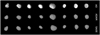 |
Fig. 2 Adaptive optics images of asteroid (3) Juno (top), the ADAM model sky projection by Viikinkoski et al. (2015) (middle), and the SAGE model (bottom) presented for the same epochs. |
3.4 (64) Angelina
The lightcurves of (64) Angelina display asymmetric and variable behavior, with amplitudes ranging from 0.04 mag to 0.42 mag, which indicates a spin axis obliquity around 90 degrees. Data from ten apparitions were used to calculate the SAGE model. The synthetic lightcurves that were generated from the shape are in good agreement with the observed ones. Although the low value of the pole’s latitude of 12° is consistentwith the previous solution by Ďurech et al. (2011) (see Table A.2 for reference), the difference of 0.0015 hours in the period is substantial. We favor our solution given our updated, richer dataset since Ďurech et al. (2011) only had dense lightcurves from three apparitions that were complemented by sparse data with uncertainties of 0.1–0.2 mag (i.e., the level of lightcurve amplitude of this target). Also, the level of the occultation fit (Fig. C.4) and the TPM support our model. The thermal data were well reproduced with sizes that are slightly larger but consistent with the ones from the occultation fitting (54 versus 50 km, see Tables 2 and A.1), and they slightly favor the same pole solution.
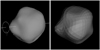 |
Fig. 3 Sky projections for the same epoch of SAGE (left) and ADAM (right) shape models of asteroid (14) Irene. Both shapes are in very good agreement. |
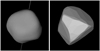 |
Fig. 4 Sky projections for the same epoch of the SAGE (left) and convex inversion (right) shape models of asteroid (68) Leto. SAGE provided a largely different and much smoother shape solution. |
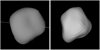 |
Fig. 5 Sky projections for the same epoch of SAGE (left) and ADAM (right) shape models of asteroid (89) Julia. A similar crater on the southern pole was reproduced by both methods. |
3.5 (68) Leto
For Leto, data from six different apparitions consisted of somewhat asymmetric lightcurves with unequally spaced minima. Amplitudes ranged from 0.10 to 0.28 mag. The angular convex shape model published previously by Hanuš et al. (2013), which was mainly based on sparse data, is compared here with a much smoother SAGE model. Their on-sky projections on the same epoch can be seen in Fig. 4. The TPM analysis did not favor any of the poles. There was only one three-chords occultation, which the models did not fit perfectly, although pole 2 was fit better this time (see Fig. C.5). Also, the occultation size of the pole 1 solution is 30 km larger than the radiometric one ( versus 121 km), with similarly large error bars, whereas the
  km size of the pole 2 solution is more consistent with the TPM and it has smaller error bars (see Table 2 and A.1).
3.6 (89) Julia
This target was shared with the VLT large program 199.C-0074 (PI: Pierre Vernazza), which obtained a rich set of well-resolved adaptive optics images using VLT/SPHERE instrument. Vernazza et al. (2018) produced a spin and shape model of (89) Julia using the ADAM algorithm on lightcurves and AO images, which enabled them to reproduce major nonconvex shape features. They identified a large impact crater that is possibly the source region of the asteroids of the Julia collisional family. The SAGE model, which is based solely on disk-integrated photometry, also reproduced the biggest crater and some of the hills present in the ADAM model (Fig. 5). Spin parameters are in very good agreement. Interestingly, lightcurve data from only four apparitions were used for both models. However, one of them spanned five months, covering a large range of phase angles that highlighted the surface features due to various levels of shadowing. Both models fit them well, but the SAGE model does slightly worse. In the occultation fitting of two multichord events from the years 2005 and 2006, some of the SAGE shape features seem too small and others seem too large, but overall we obtain a size (138 km) that is almost identical to the ADAM model size (139 ± 3 km). The TPM requires a larger size (150 ± 10 km) for this model, but it is still consistent within the error bars.
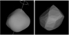 |
Fig. 6 Sky projections for the same epoch of SAGE (left) and convex inversion (right) shape models of asteroid (381) Myrrha. SAGE model is similar to the one from convex inversion, but it is less angular. |
3.7 (114) Kassandra
The lightcurves of Kassandra from nine apparitions (although only six have distinct geometries) showed sharp minima of uneven depths and had amplitudes from 0.15 to 0.25 mag. The SAGE shape model looks quite irregular, with a deep polar crater. It does not resemble the convex model by Ďurech et al. (2018b), which is provided with a warning of its wrong inertia tensor. Nevertheless, the spin parameters of both solutions roughly agree. The SAGE model fits the lightcurves well, except for three cases involving the same ones that the convex model also failed to fit. This might indicate that they are burdened with some instrumental or other systematic errors. Unfortunately, no well-covered stellar occultations are available for Kassandra, so the only size determination could be done here by TPM (see Table A.1). Despite the substantial irregularity of the SAGE shape model, the spherical shape gives a similarly good fit to the thermal data.
3.8 (145) Adeona
Despite the fact that the available set of lightcurves came from nine apparitions, their unfortunate grouping resulted in only five distinct viewing aspects of this body. The small amplitudes (0.04–0.15 mag) displayed by this target were an additional hindering factor. Therefore, there was initially a controversy as to whether its period is close to 8.3 or 15 h. It was resolved by good quality data obtained by Pilcher (2010), which is in favor of the latter. SAGE model fit most of the lightcurves well, but it had problems with some where visible deviations are apparent. This is the first model of this target, so there is not a previous model with which to compare it. The SAGE model looks almost spherical without notable shape features, so, as expected, the spherical shape provided a similarly good fit to the thermal data. The model fits the only available stellar occultation very well, which has the volume equivalent diameter of  km.
km.
3.9 (297) Caecilia
There were data from nine apparitions available for Caecilia, which were well spread in ecliptic longitude. The lightcurves displayed mostly regular, bimodal character of 0.15–0.28 mag amplitudes. The previous model by Hanuš et al. (2013) was created on amuch more limited data set, with dense lightcurves covering only 1/3 of the orbit, which was supplemented by sparse data. So, as expected, that shape model is rather crude compared to the SAGE model. Nonetheless, the period and pole orientation is in good agreement between the two models, and there were similar problems with both shapes when fitting some of the lightcurves.
No stellar occultations by Caecilia are available with a sufficient number of chords, so the SAGE model was only scaled here by TPM (see Table A.1). However, the diameter provided here is merely the best-fitting value since the number of thermal IR data is too low to provide a realistic uncertainty estimate.
3.10 (308) Polyxo
The available lightcurve data set has been very limited for Polyxo, so no model could have been previously constructed. However, thanks to an extensive SBNAF observing campaign and the observations collected through GaiaGOSA, we now have data from six apparitions, covering five different aspects. The lightcurves were very irregular and had a small amplitude (0.08–0.22 mag), often displaying three maxima per period. To check the reliability of our solution, we determined the model based on the simple lightcurve inversion method. Then, we compared the results with those from the SAGE method. All the parameters are in agreement within the error bars between the convex and SAGE models. Still, the SAGE shape model looks rather smooth, with only small irregularities, and it fits the visible lightcurves reasonably well. There were three multichord occultations for Polyxo in PDS obtained in 2000, 2004, and 2010. Both pole solutions fit them at a good level (see Fig. C.8 for details) and produced mutually consistent diameters derived from each of the events separately (125−133 km, see Table 2). The TPM diameter (139 km) is slightly larger though. However, in this case, there are not enough thermal data to provide a realistic estimate of the error bars.
3.11 (381) Myrrha
In the case of Myrrha, there were data from seven apparitions, but only five different viewing aspects. The lightcurves displayed a regular shape with a large amplitude from 0.3 to 0.36 mag. Thanks to the observing campaign that was conducted in the framework of the SBNAF project and the GaiaGOSA observers, we were able to determine the shape and spin state. Without the new data, the previous set of viewing geometries would have been limited to only 1/3 of the Myrrha orbit, and the earlier model by Hanuš et al. (2016) was constructed on dense lightcurves supplemented with sparse data. As a consequence, the previous model looks somewhat angular (cf. both shapes in Fig. 6). Due to a very high inclination of the pole to the ecliptic plane (high value of |β|), two potential mirror pole solutions were very close to each other. As a result, an unambiguous solution for the pole position was found. A very densely covered stellar occultation was available, although some of the 25 chords are mutually inconsistent and burdened with large uncertainties (see Fig. C.9). In the thermal IR, the SAGE model of Myrrha fits the rich data set better than the sphere with the same pole, giving a larger diameter. The obtained diameter has a small estimated error bar (131 ± 4 km) and it is in close agreement with the size derived from the occultation fitting of timing chords ( km).
km).
3.12 (441) Bathilde
Seven different viewing geometries from ten apparitions were available for Bathilde. The amplitude of the lightcurves varied from 0.08 to 0.22 mag. Similarly, as in a few previously described cases, a previous model of this target based on sparse and dense data was available (Hanuš et al. 2013). The new SAGE shape fit additional data and it has a smoother shape.
Shapes for both pole solutions fit the only available occultation well, and the resulting size (around 76 km) is in agreement with the size from TPM (72 ± 2 km). Interestingly, the second solution for the pole seems to be rejected by TPM, and the favored one fits thermal data much better than in the corresponding sphere. The resulting diameter is larger than the one obtained from AKARI, SIMPS, and WISE (see Tables 2, A.1 and A.2 for comparison).
3.13 (721) Tabora
Together with new observations that were gathered by the SBNAF observing campaign, we have data from five apparitions for Tabora. Amplitudes ranged from 0.19 to 0.50 mag, and the lightcurves were sometimes strongly asymmetric, with extrema at different levels. A model of Tabora has been published recently and it is based on joining sparse data in the visible with WISE thermal data (bands W3 and W4, Ďurech et al. 2018a), but it does not have an assigned scale. The resulting shape model is somewhat angular, but it is in agreement with the SAGE model with respect to spin parameters. Stellar occultations are also lacking for Tabora, and the TPM only gave a marginally acceptable fit (χ2 = 1.4 for pole 1) to the thermal data, which is nonetheless much better than the sphere. Thus, the diameter error bar, in this case, is not optimal (~ 6%) and additional IR data and/or occultations would be required to provide a better constrained volume.
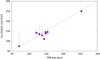 |
Fig. 7 Set of average occultation diameters vs. diameters from TPM. The straight line is y = x. |
4 Conclusions
Here, we derived spin and shape models of 13 asteroids that were selected from Gaia mass targets, using only photometric lightcurves. It is generally possible to recover major shape features of main belt asteroids, but other techniques, such as direct images or adaptive optics, should be used to confirm the main features. We scaled our shape models by using stellar occultation records and TPM. The results obtained from both techniques are usually in good agreement, what can be seen in Fig. 7. In many ways, the stellar occultation fitting and thermophysical modeling are complementary to each other. In most cases, occultation chords match the silhouette within the error bars and rough diameters are provided. Also, thermophysical modeling resulted in more precise size determinations, thus additionally constraining the following thermal parameters: thermal inertia and surface roughness (see Table A.1). The diameters based on occultation fitting of complex shape models, inaccurate as they may seem here when compared to those from TPM, still reflect the dimensions of real bodies better than the commonly used elliptical approximation of the shape projection. The biggest advantage of scaling 3D shape models by occultations is that this procedure provides volumes of these bodies, unlike the fitting of 2D elliptical shape approximations, which only provides the lower limit for the size of the projection ellipse.
Resulting volumes, especially those with relatively small uncertainty, are going to be a valuable input for the density determinations of these targets once the mass values from the Gaia astrometry become available. In the cases where only convex solutions were previously available, nonconvex solutions created here will lead to more precise volumes, and consequently better constrained densities. In a few cases, our solutions are the first in the literature. The shape models, spin parameters, diameters, volumes, and corresponding uncertainties derived here are already available on the ISAM webpage.
Acknowledgements
The research leading to these results has received funding from the European Union’s Horizon 2020 Research and Innovation Programme, under Grant Agreement no 687378 (SBNAF). Funding for the Kepler and K2 missions is provided by the NASA Science Mission directorate. L.M. was supported by the Premium Postdoctoral Research Program of the Hungarian Academy of Sciences. The research leading to these results has received funding from the LP2012-31 and LP2018-7 Lendület grants of the Hungarian Academy of Sciences. This project has been supported by the Lendület grant LP2012-31 of the Hungarian Academy of Sciences and by the GINOP-2.3.2-15-2016-00003 grant of the Hungarian National Research, Development and Innovation Office (NKFIH). TRAPPIST-South is a project funded by the Belgian Fonds de la Recherche Scientifique (F.R.S.-FNRS) under grant FRFC 2.5.594.09.F. TRAPPIST-North is a project funded by the University of Liège, and performed in collaboration with Cadi Ayyad University of Marrakesh. E.J. is a FNRS Senior Research Associate. “The Joan Oró Telescope (TJO) of the Montsec Astronomical Observatory (OAdM) is owned by the Catalan Government and operated by the Institute for Space Studies of Catalonia (IEEC).” “This article is based on observations made with the SARA telescopes (Southeastern Association for Research in Astronomy), whose node is located at the Kitt Peak National Observatory, AZ under the auspices of the National Optical Astronomy Observatory (NOAO).” “This project uses data from the SuperWASP archive. The WASP project is currently funded and operated by Warwick University and Keele University, and was originally set up by Queen’s University Belfast, the Universities of Keele, St. Andrews, and Leicester, the Open University, the Isaac Newton Group, the Instituto de Astrofisica de Canarias, the South African Astronomical Observatory, and by STFC.” “This publication makes use of data products from the Wide-field Infrared Survey Explorer, which is a joint project of the University of California, Los Angeles, and the Jet Propulsion Laboratory/California Institute of Technology, funded by the National Aeronautics and Space Administration.” The work of TSR was carried out through grant APOSTD/2019/046 by Generalitat Valenciana (Spain)
Appendix A Additional tables
Summary of TPM results, including the minimum reduced chi-squared ( ), the best-fitting diameter (D) and corresponding 1σ statistical error bars, and the number of IR data that were modeled (NIR).
Results from the previous solutions available in the literature.
Appendix B TPM plots and comments
The data we used was collected in the SBNAF infrared database4. In this section, we provide observation-to-model ratio (OMR) plots produced for the TPM analysis. Whenever there was a thermal lightcurve available within the data set of a target, this was also plotted (see Table A.1). In general, IRAS data have larger error bars, carry lower weights, and, therefore, their OMRs tend to present larger deviations from one. On a few occasions, some or all of them were even removed from the χ2 optimization, as indicated in the corresponding figure caption. To save space, we only include the plots for one of the mirror solutions either because the TPM clearly rejected the other one or because the differences were so small that the other set of plots are redundant. Either way, that information is given in Table A.1. Table B.1 links each target to its corresponding plots in this section.
Targets and references to the relevant figures.
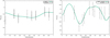 |
Fig. B.1 W4 data and model of thermal lightcurves that were generated with the best-fitting thermal parameters and size. Left: (64) Angelina’s SAGE pole 1 model. Right: (68) Leto, also Pole 1. |
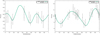 |
Fig. B.2 Left: (114) Kassandra. Right: (381) Myrrha. |
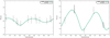 |
Fig. B.3 Left: (441) Bathilde. Right: (721) Tabora. |
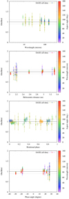 |
Fig. B.4 (3) Juno (from top to bottom): observation-to-model ratios versus wavelength, heliocentric distance, rotational phase, and phase angle. The color bar either corresponds to the aspect angle or to the wavelength at which each observation was taken. There are some systematics in the rotational phase plot, which indicate there could be some small artifacts in the shape. |
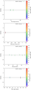 |
Fig. B.5 (14) Irene (from top to bottom): observation-to-model ratios versus wavelength, heliocentric distance, rotational phase, and phase angle. The plots that correspond to the pole 2 solution are very similar. |
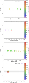 |
Fig. B.6 (20) Massalia. The O01 label indicates that the IRAS data were removed from the analysis, in this case because their qualitywas too poor. |
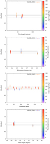 |
Fig. B.7 (64) Angelina. Pole 1 was favored in this case because it provided a significantly lower minimum χ2. The O01 label indicates that the very few MSX were clear outliers and were removed from the analysis. |
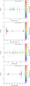 |
Fig. B.8 (68) Leto. The two mirror solutions fitted the data statistically equally well. |
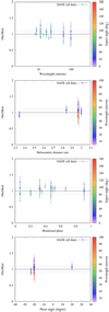 |
Fig. B.9 (89) Julia. The SAGE model provided a formally acceptable fit to the data (see Table A.1) but the optimum thermal inertia (150 SI units) is higher than expected for such a large main-belt asteroid. It is probably an artefact and manifests itself in the strong slope in the wavelength plot. The bias could be caused by two possible factors: We did not consider the dependence of thermal inertia with temperature (see e.g., Marsset et al. 2017; Rozitis et al. 2018) and the data were taken over a wide range of heliocentric distances; the thermal inertia is not well constrained because we have very few observations at positive phase angles. |
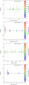 |
Fig. B.10 (114) Kassandra. |
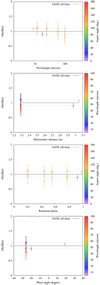 |
Fig. B.11 (145) Adeona. |
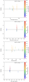 |
Fig. B.12 (297) Caecilia. There is not good phase angle coverage. There were not enough data to provide realistic error bars for the size. More thermal IR data are clearly needed. |
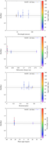 |
Fig. B.13 (308) Polyxo. |
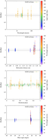 |
Fig. B.14 (381) Myrrha. There are some waves in the rotational phase plot that suggest small shape issues (see also Fig. B.2), but overall, the fit has a low χ2 and is muchbetter than the sphere with the same spin axis. |
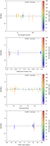 |
Fig. B.15 (441) Bathilde. |
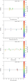 |
Fig. B.16 (721) Tabora. |
Appendix C Stellar occultation records fitting
In this section we present the model fit to stellar occultation chords.
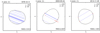 |
Fig. C.1 Shape model fitting to stellar occultations by 3 Juno. |
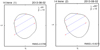 |
Fig. C.2 Shape model fitting to stellar occultations by 14 Irene. |
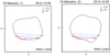 |
Fig. C.3 Shape model fitting to stellar occultations by 20 Massalia. |
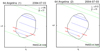 |
Fig. C.4 Shape model fitting to stellar occultations by 64 Angelina. |
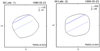 |
Fig. C.5 Shape model fitting to stellar occultations by 68 Leto. |
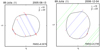 |
Fig. C.6 Shape model fitting to stellar occultations by 89 Julia. |
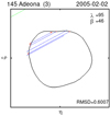 |
Fig. C.7 Shape model fitting to stellar occultations by 145 Adeona. |
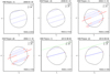 |
Fig. C.8 Shape model fitting to stellar occultations by 308 Polyxo. |
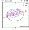 |
Fig. C.9 Shape model fitting to stellar occultations by 381 Myrrha. |
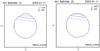 |
Fig. C.10 Shape model fitting to stellar occultations by 441 Bathilde. |
References
- Alí-Lagoa, V., Lionni, L., Delbo, M., et al. 2014, A&A, 561, A45 [NASA ADS] [CrossRef] [EDP Sciences] [Google Scholar]
- Alí-Lagoa, V., Müller, T. G., Usui, F., Hasegawa, S. 2018, A&A, 612, A85 [NASA ADS] [CrossRef] [EDP Sciences] [Google Scholar]
- Bartczak, P., & Dudziński, G. 2018, MNRAS, 473, 5050 [NASA ADS] [CrossRef] [Google Scholar]
- Bartczak, P., & Dudziński, G. 2019, MNRAS, 485, 2431 [NASA ADS] [CrossRef] [Google Scholar]
- Carry, B. 2012, Planet. Space Sci., 73, 98 [NASA ADS] [CrossRef] [Google Scholar]
- Carry, B., Merline, W. J., Kaasalainen, M., et al. 2010, BAAS, 42, 1050 [NASA ADS] [Google Scholar]
- Delbo, M., & Harris, A. W. 2002, Meteorit. Planet. Sci., 37, 1929 [NASA ADS] [CrossRef] [Google Scholar]
- Delbo, M., Mueller, M., Emery, J. P., Rozitis, B., & Capria, M. T. 2015, Asteroids IV, eds. P. Michel, F. E. DeMeo, & W. F. Bottke (Tucson: University of Arizona Press), 107 [Google Scholar]
- Dunham, D. W., Herald, D., Frappa, E., et al. 2016, NASA Planetary Data System, 243, EAR [Google Scholar]
- Ďurech, J., Sidorin, V., Kaasalainen, M. 2010, A&A, 513, A46 [NASA ADS] [CrossRef] [EDP Sciences] [Google Scholar]
- Ďurech, J., Kaasalainen, M., Herald, D., et al. 2011, Icarus, 214, 652 [NASA ADS] [CrossRef] [Google Scholar]
- Ďurech, J., Carry, B., Delbo, M., Kaasalainen, M., Viikinkoski, M. 2015, Asteroids IV, eds. P. Michel, F. E. DeMeo, & W. F. Bottke (Tucson: University of Arizona Press), 183 [Google Scholar]
- Ďurech, J., Hanuš, J., Alí-Lagoa, V., et al. 2018a A&A, 617, A57 [NASA ADS] [CrossRef] [EDP Sciences] [Google Scholar]
- Ďurech, J., Hanuš, J., Broz, M., et al. 2018b, Icarus, 304, 101 [NASA ADS] [CrossRef] [Google Scholar]
- Grice, J., Snodgrass, C., Green, S., Parley, N., & Carry, B. 2017, in Asteroids, Comets, meteors: ACM 2017 [Google Scholar]
- Hanuš, J., Ďurech, J., Broz, M., et al. 2013, A&A, 551, A67 [NASA ADS] [CrossRef] [EDP Sciences] [Google Scholar]
- Hanuš, J., Ďurech, J., Oszkiewicz, D. A., et al. 2016, A&A, 586, A108 [NASA ADS] [CrossRef] [EDP Sciences] [Google Scholar]
- Harris, A. W.; Lagerros, J. S. V. 2002, Asteroids III, eds. W. F. Bottke Jr., A. Cellino, P. Paolicchi, & R. P. Binzel (Tucson: University of Arizona Press), 205 [Google Scholar]
- Jehin, E., Gillon, M., Queloz, D., et al. 2011, The Messenger, 145, 2 [NASA ADS] [Google Scholar]
- Kaasalainen, M., Torppa, J., & Piironen, J. 2002, Icarus, 159, 369 [NASA ADS] [CrossRef] [Google Scholar]
- Lagerros, J. S.V. 1996, A&A, 310, 1011 [NASA ADS] [Google Scholar]
- Lagerros, J. S.V. 1998, A&A, 332, 1123 [NASA ADS] [Google Scholar]
- Mainzer, A. K., Bauer, J. M., Cutri, R. M., et al. 2016, NASA Planetary Data System, id. EAR-A-COMPIL-5-NEOWISEDIAM-V1.0 [Google Scholar]
- Marciniak, A., Bartczak, P., Santana-Ros, T., et al. 2012, A&A, 545, A131 [NASA ADS] [CrossRef] [EDP Sciences] [Google Scholar]
- Marciniak, A., Bartczak, P., Müller, T. G., et al. 2018, A&A, 610, A7 [NASA ADS] [CrossRef] [EDP Sciences] [Google Scholar]
- Marciniak, A., Alí-Lagoa, V., Müller, T. G., et al. 2019, A&A, 625, A139 [NASA ADS] [CrossRef] [EDP Sciences] [Google Scholar]
- Marsset, M., Carry, B., Dumas, C., et al. 2017, A&A, 604, A64 [NASA ADS] [CrossRef] [EDP Sciences] [Google Scholar]
- Michałowski, T., Velichko, F. P., Di Martino, M., et al. 1995, Icarus, 118, 292 [NASA ADS] [CrossRef] [Google Scholar]
- Morbidelli, A., Bottke, W. F., Nesvorny, D., Levison, H. F. 2009, Icarus, 204, 558 [NASA ADS] [CrossRef] [Google Scholar]
- Mouret, S., Hestroffer, D., & Mignard, F., 2007, A&A, 472, 1017 [NASA ADS] [CrossRef] [EDP Sciences] [Google Scholar]
- Müller, T. G. 2002, Meteorit. Planet. Sci., 37, 1919 [NASA ADS] [CrossRef] [Google Scholar]
- Müller, T. G., & Lagerros, J. S. V. 1998, A&A, 338, 340 [NASA ADS] [Google Scholar]
- Müller, T. G., Herschel Calibration Steering Group, & ASTRO-F Calibration Team 2005, ESA report [Google Scholar]
- Müller, T., Balog, Z., Nielbock, M., et al. 2014, Exp. Astron., 37, 253 [NASA ADS] [CrossRef] [Google Scholar]
- Müller, T. G., Marciniak, A., Kiss, Cs, et al. 2018, Adv. Space Res., 62, 2326 [NASA ADS] [CrossRef] [Google Scholar]
- Oszkiewicz, D.A., Muinonen, K., Bowell, E., et al. 2011, J. Quant. Spectr. Rad. Transf., 112, 1919 [NASA ADS] [CrossRef] [Google Scholar]
- Pilcher, F. 2010, Minor Planet Bull., 37, 148 [NASA ADS] [Google Scholar]
- Rozitis, B., & Green, S. F. 2014, A&A, 568, A43 [NASA ADS] [CrossRef] [EDP Sciences] [Google Scholar]
- Rozitis, B., Green, S. F., MacLennan, E., et al. 2018, MNRAS, 477, 1782 [NASA ADS] [CrossRef] [Google Scholar]
- Rubincam, D. P. 2001, Icarus, 148, 2 [Google Scholar]
- Santana-Ros, T., Marciniak, A., & Bartczak, P. 2016, Minor Planet Bull., 43, 205 [NASA ADS] [Google Scholar]
- Scott, E. R. D., Keil, K., Goldstein, J. I., et al. 2015, Asteroids IV, eds. F. E. DeMeo, & W. F. Bottke (Tucson: University of Arizona Press), 573 [Google Scholar]
- Slivan, S. M. 2002, Nature, 419, 6902 [NASA ADS] [CrossRef] [PubMed] [Google Scholar]
- Szabó, Gy. M., Pál, A., Kiss, Cs., et al. 2017, A&A, 599, A44 [NASA ADS] [CrossRef] [EDP Sciences] [Google Scholar]
- Tedesco, E. F., Cellino, A., & Zappalá, V. 2005, AJ, 129, 2869 [NASA ADS] [CrossRef] [Google Scholar]
- Usui, F., Kuroda, S., Müller, t. G., et al. 2011, PASJ, 63, 1117 [NASA ADS] [CrossRef] [Google Scholar]
- Veres, P., Jedicke, R., Fitzsimmons, A., et al. 2015, Icarus, 261, 34 [NASA ADS] [CrossRef] [Google Scholar]
- Vernazza, P., Broz, M., Drouard, A., et al. 2018, A&A, 618, A154 [NASA ADS] [CrossRef] [EDP Sciences] [Google Scholar]
- Vernazza, P., Jorda, L., Ševeček, P., et al. 2019, Nat. Astron., 477V [Google Scholar]
- Viikinkoski, M., Kaasalainen, M., Durech, J., et al. 2016 A&A, 581, L3 [Google Scholar]
- Viikinkoski, M., Hanus, J., Kaasalainen, M., Marchis, F., & Durech, J. 2017, A&A, 607, A117 [NASA ADS] [CrossRef] [EDP Sciences] [Google Scholar]
- Vokrouhlický, D., Nesvorny, D., & Bottke, W. F. 2003, Nature, 425, 6954 [Google Scholar]
- Vokrouhlický, D., Bottke, W. F., Chesley, S. R., et al. 2015, Asteroids IV, eds. P. Michel, F. E. DeMeo, & W. F. Bottke, (Tucson: University of Arizona Press), 895, 509 [NASA ADS] [Google Scholar]
- Wright, E. L., Eisenhardt, P. R. M., Mainzer, A. K., et al. 2010, AJ, 140, 1868 [NASA ADS] [CrossRef] [Google Scholar]
All Tables
Spin parameters of asteroid models obtained in this work, with their uncertainty values.
Summary of TPM results, including the minimum reduced chi-squared (), the best-fitting diameter (D) and corresponding 1σ statistical error bars, and the number of IR data that were modeled (NIR).
All Figures
|
Fig. 1 Observer-centered ecliptic longitude of asteroid (441) Bathilde at apparitions with well covered lightcurves. |
| In the text | |
|
Fig. 2 Adaptive optics images of asteroid (3) Juno (top), the ADAM model sky projection by Viikinkoski et al. (2015) (middle), and the SAGE model (bottom) presented for the same epochs. |
| In the text | |
|
Fig. 3 Sky projections for the same epoch of SAGE (left) and ADAM (right) shape models of asteroid (14) Irene. Both shapes are in very good agreement. |
| In the text | |
|
Fig. 4 Sky projections for the same epoch of the SAGE (left) and convex inversion (right) shape models of asteroid (68) Leto. SAGE provided a largely different and much smoother shape solution. |
| In the text | |
|
Fig. 5 Sky projections for the same epoch of SAGE (left) and ADAM (right) shape models of asteroid (89) Julia. A similar crater on the southern pole was reproduced by both methods. |
| In the text | |
|
Fig. 6 Sky projections for the same epoch of SAGE (left) and convex inversion (right) shape models of asteroid (381) Myrrha. SAGE model is similar to the one from convex inversion, but it is less angular. |
| In the text | |
|
Fig. 7 Set of average occultation diameters vs. diameters from TPM. The straight line is y = x. |
| In the text | |
|
Fig. B.1 W4 data and model of thermal lightcurves that were generated with the best-fitting thermal parameters and size. Left: (64) Angelina’s SAGE pole 1 model. Right: (68) Leto, also Pole 1. |
| In the text | |
|
Fig. B.2 Left: (114) Kassandra. Right: (381) Myrrha. |
| In the text | |
|
Fig. B.3 Left: (441) Bathilde. Right: (721) Tabora. |
| In the text | |
|
Fig. B.4 (3) Juno (from top to bottom): observation-to-model ratios versus wavelength, heliocentric distance, rotational phase, and phase angle. The color bar either corresponds to the aspect angle or to the wavelength at which each observation was taken. There are some systematics in the rotational phase plot, which indicate there could be some small artifacts in the shape. |
| In the text | |
|
Fig. B.5 (14) Irene (from top to bottom): observation-to-model ratios versus wavelength, heliocentric distance, rotational phase, and phase angle. The plots that correspond to the pole 2 solution are very similar. |
| In the text | |
|
Fig. B.6 (20) Massalia. The O01 label indicates that the IRAS data were removed from the analysis, in this case because their qualitywas too poor. |
| In the text | |
|
Fig. B.7 (64) Angelina. Pole 1 was favored in this case because it provided a significantly lower minimum χ2. The O01 label indicates that the very few MSX were clear outliers and were removed from the analysis. |
| In the text | |
|
Fig. B.8 (68) Leto. The two mirror solutions fitted the data statistically equally well. |
| In the text | |
|
Fig. B.9 (89) Julia. The SAGE model provided a formally acceptable fit to the data (see Table A.1) but the optimum thermal inertia (150 SI units) is higher than expected for such a large main-belt asteroid. It is probably an artefact and manifests itself in the strong slope in the wavelength plot. The bias could be caused by two possible factors: We did not consider the dependence of thermal inertia with temperature (see e.g., Marsset et al. 2017; Rozitis et al. 2018) and the data were taken over a wide range of heliocentric distances; the thermal inertia is not well constrained because we have very few observations at positive phase angles. |
| In the text | |
|
Fig. B.10 (114) Kassandra. |
| In the text | |
|
Fig. B.11 (145) Adeona. |
| In the text | |
|
Fig. B.12 (297) Caecilia. There is not good phase angle coverage. There were not enough data to provide realistic error bars for the size. More thermal IR data are clearly needed. |
| In the text | |
|
Fig. B.13 (308) Polyxo. |
| In the text | |
|
Fig. B.14 (381) Myrrha. There are some waves in the rotational phase plot that suggest small shape issues (see also Fig. B.2), but overall, the fit has a low χ2 and is muchbetter than the sphere with the same spin axis. |
| In the text | |
|
Fig. B.15 (441) Bathilde. |
| In the text | |
|
Fig. B.16 (721) Tabora. |
| In the text | |
|
Fig. C.1 Shape model fitting to stellar occultations by 3 Juno. |
| In the text | |
|
Fig. C.2 Shape model fitting to stellar occultations by 14 Irene. |
| In the text | |
|
Fig. C.3 Shape model fitting to stellar occultations by 20 Massalia. |
| In the text | |
|
Fig. C.4 Shape model fitting to stellar occultations by 64 Angelina. |
| In the text | |
|
Fig. C.5 Shape model fitting to stellar occultations by 68 Leto. |
| In the text | |
|
Fig. C.6 Shape model fitting to stellar occultations by 89 Julia. |
| In the text | |
|
Fig. C.7 Shape model fitting to stellar occultations by 145 Adeona. |
| In the text | |
|
Fig. C.8 Shape model fitting to stellar occultations by 308 Polyxo. |
| In the text | |
|
Fig. C.9 Shape model fitting to stellar occultations by 381 Myrrha. |
| In the text | |
|
Fig. C.10 Shape model fitting to stellar occultations by 441 Bathilde. |
| In the text | |
Current usage metrics show cumulative count of Article Views (full-text article views including HTML views, PDF and ePub downloads, according to the available data) and Abstracts Views on Vision4Press platform.
Data correspond to usage on the plateform after 2015. The current usage metrics is available 48-96 hours after online publication and is updated daily on week days.
Initial download of the metrics may take a while.