| Issue |
A&A
Volume 636, April 2020
|
|
|---|---|---|
| Article Number | A114 | |
| Number of page(s) | 11 | |
| Section | Interstellar and circumstellar matter | |
| DOI | https://doi.org/10.1051/0004-6361/201935386 | |
| Published online | 28 April 2020 | |
Deep search for hydrogen peroxide toward pre- and protostellar objects
Testing the pathway of grain surface water formation
1
Institute of Physics, University Kassel,
Heinrich-Plett Str. 40,
34132
Kassel,
Germany
e-mail: This email address is being protected from spambots. You need JavaScript enabled to view it.
2
Max-Planck-Institute for Extraterrestrial Physics (MPE),
Giessenbachstraße 1,
85748
Garching,
Germany
3
Laboratory for Astrophysics, Leiden Observatory, Leiden University,
PO Box 9513,
2300 RA
Leiden, The Netherlands
4
Max-Planck-Institut for Radio Astronomy (MPIfR),
Auf dem Hügel 69,
53121
Bonn,
Germany
Received:
1
March
2019
Accepted:
14
March
2020
Abstract
Context. In the laboratory, hydrogen peroxide (HOOH) was proven to be an intermediate product in the solid-state reaction scheme that leads to the formation of water on icy dust grains. When HOOH desorbs from the icy grains, it can be detected in the gas phase. In combination with water detections, it may provide additional information on the water reaction network. Hydrogen peroxide has previously been found toward ρ Oph A. However, further searches for this molecule in other sources failed. Hydrogen peroxide plays a fundamental role in the understanding of solid-state water formation and the overall water reservoir in young stellar objects (YSOs). Without further HOOH detections, it is difficult to assess and develop suitable chemical models that properly take into account the formation of water on icy surfaces.
Aims. The objective of this work is to identify HOOH in YSOs and thereby constrain the grain surface water formation hypothesis.
Methods. Using an astrochemical model based on previous work in combination with a physical model of YSOs, the sources R CrA-IRS 5A, NGC C1333-IRAS 2A, L1551-IRS 5, and L1544 were identified as suitable candidates for an HOOH detection. Long integration times on the APEX 12 m and IRAM 30 m telescopes were applied to search for HOOH signatures in these sources.
Results. None of the four sources under investigation showed convincing spectral signatures of HOOH. The upper limit for HOOH abundance based on the noise level at the frequency positions of this molecule for the source R CrA-IRS 5A was close to the predicted value. For NGC 1333-IRAS 2A, L1544, and L1551-IRS 5, the model overestimated the hydrogen peroxide abundances.
Conclusions. HOOH remains an elusive molecule. With only one secure cosmic HOOH source detected so far, namely ρ Oph A, the chemical model parameters for this molecule cannot be sufficiently well determined or confirmed in existing models. Possible reasons for the nondetections of HOOH are discussed.
Key words: ISM: molecules / ISM: abundances / methods: observational / stars: formation / submillimeter: ISM / astrochemistry
© ESO 2020
1 Introduction
Water is the essence of life and is one of the most relevant molecules in the Universe. In star formation processes, H2O plays an important role as coolant; in dense cold regions, water is the dominant constituent in ices coating cosmic grains; and generally, water can be used as a valuable physical diagnostic and evolutionary tracer (van Dishoeck et al. 2011). Its origin and abundance in space is at the core of fundamental questions that still lack conclusive answers. Three reaction schemes are commonly used to explain water formation in space (van Dishoeck et al. 2013; Hollenbach et al. 2009). In hot or radiation-exposed environments, gas-phase reactions dominate that are either based on high temperature (1) or ion-molecule reactions (2). In cold and radiatively well-shielded regions where ices form on cold dust grains, solid-state reactions (3) are at play. The latter mechanism is believed to dominate in the environments of star-forming regions. Dedicated observing programs such as the Herschel-WISH program (van Dishoeck et al. 2011) have investigated the abundance and occurrence of water in our Universe and in our local galactic environment. In addition, laboratory data of chemical processes in interstellar ice analogs became available that helped to better understand the mechanisms of water formation on interstellar dust surfaces (Ioppolo et al. 2010). Laboratory studies showed that hydrogen peroxide (HOOH) acts as a prominent intermediate in the hydrogenation chain from oxygen allotropes (O, O2, and O3) to the formation of water (Ioppolo et al. 2008; Miyauchi et al. 2008; Oba et al. 2009; Dulieu et al. 2010; Cuppen et al. 2010; Romanzin et al. 2011). This also means that HOOH has the potential of acting as a tracer of solid-state reactions that result in the formation of water. This depends on the amount of HOOH that is present in the ice because it may fully react to form water, and it depends on the efficiency with which HOOH can be released into the gas phase after it is formed, for instance, through reactive desorption or dissociative desorption processes. In addition, the amount of observable HOOH may be reduced by gas phase processes that consume HOOH once it is released from the solid. The first point, that is the amount of solid-state HOOH, has been addressed by Smith et al. (2011) by investigating interstellar ices at 3.5, 7.0, and 11.3 μm where HOOH can be distinguished from water ices; see also Boudin et al. (1998). However, no conclusive evidence for HOOH as grain mantle constituent could be reported. At best, the 3.47 μm feature at the shoulder of the long-wavelength wing of the 3.08 μm water O–H stretching feature might be assumed to originate from HOOH (but possibly also from other molecules) and might thus be used to infer an upper limit, which would then be between 2 and 17%. However, already in 2011, gas-phase HOOH was identified toward the star-formingregion ρ Oph A (Bergman et al. 2011a). Du et al. (2012) developed a detailed model based on chemical surface reactions and subsequent desorption processes to explain these observations. They also predicted that HO2 exists in ρ Oph A in sufficient amounts that were subsequently detected by Parise et al. (2012). Based on these first successes, a survey toward various inter- and circumstellar environments, including star-forming regions at various phases of stellar evolution, was started by Parise and colleagues to search for further sources of hydrogen peroxide. Surprisingly, it was not possible to identify HOOH in any of these targets (Parise et al. 2014). Liseau & Larsson (2015) reported a tentative detection of hydrogen peroxide toward OMC-1, but because the millimeter spectrum in this source is very dense, a firm assignment is still pending. Because water can be seen in many star-forming regions, including those investigated by Parise et al. (2014), it remains puzzling why HOOH is so difficult to observe. Parise et al. argued that ρ Oph A appears to be a somewhat special source with favorable conditions for an HOOH detection mainly because the bulk of gas can be found under constant conditions at moderate temperatures of around 20–30 K. The heating source responsible for these temperatures is the nearby star S1 (a close binary system of the classes B4 and K). It has also been pointed out that sources in which the molecule O2 has been observed would be ideal candidates for HOOH detections (Liseau & Larsson 2015) because molecular oxygen is a direct precursor molecule for HOOH on grain surfaces (Cuppen et al. 2010). However, O2 is difficult to detect, and it is commonly believed that it is not a major repository of oxygen in molecular clouds. In only two sources has molecular oxygen been identified so far, namely ρ Oph A and Orion A (Larsson et al. 2007; Liseau et al. 2012; Goldsmith et al. 2011; Chen et al. 2014), and many further attempts to find it in the gas phase have failed (Goldsmith et al. 2000; Melnick & Bergin 2005; Yıldız et al. 2013; Wirström et al. 2016), as did the attempts to find it in solid form (Van den Bussche et al. 1999; Tielens 2000).
In the model by Du et al. (2012) a desorption mechanism is included that is based on the release of excess energy during the molecule formation. This concept has also been applied by Cazaux et al. (2016) and Minissale et al. (2016). Initially, and already including gas- and solid-phase reactions, Du et al. (2012) constrained themselves to stationary and constant physical conditions in their model. Later, they applied the model to account for spherical symmetric problems such as in NGC 1333-IRAS 4A (Parise et al. 2014). In the latter case, the HOOH nondetection disagrees with their prediction, but at the same time, their analysis emphasized the critical role of the local physical conditions (e.g., density and temperature) and age of the source, neither of which were well determined. Their model has therefore not been unequivocally confirmed so far.
Our aim is to estimate the HOOH abundance during the early phases of young stellar objects (YSOs) by combining the results of the chemical model from Du et al. (2012) with the assumption of a spherical gradient distribution of the density and temperature of these sources. YSOs in their various phases can be very complicated objects geometrically. However, for many purposes, the assumption of spherical symmetry with density and temperature gradients that can be determined by spectral energy distribution (SED) analysis is often assumed to be sufficient to obtain good estimates of key parameters of the system (Ivezic & Elitzur 1997; Schoeier et al. 2002; Kristensen et al. 2012). We therefore combined the chemical model from Du et al. (2012) with simple geometrical assumptions of the YSO in our model. This “gradient model” will be described elsewhere (Fuchs et al. 2020). In brief, because the model assumes spherical symmetry, the YSO is divided into concentric shells, each of which has constant density and temperature. The density and temperature of each shell i at radius rshell, i is given by the functions  and
and  , with p and b being specific source parameters that have been determined from SED observations. In each shell the chemistry starts with the same initial chemical composition, but then evolves differently over time according to the chemical model given by Du et al. (2012). The chemical model includes gas-phase and surface reactions, but particular attention was paid to the role of surface reactions, that is, the HOOH reaction pathway, in the water formation process. In this model, HOOH and O2 are mainly formed on grain surfaces by hydrogenation of molecular oxygen via H+O2 →O2H, with the subsequent reactions H+O2H →H2O2 and H+H2O2 →H2O + OH. Alternative surface reaction routes are also considered, such as H + O →OH and H+OH →H2O, but they do not result in comparable amounts of HOOH or H2O. Using our gradient model, we predict the gas-phase abundance of HOOH in the close-by YSOs L1551-IRS 5, R CrA-IRS 5A, and NGC 1333-IRAS 2A, as well as in the pre-stellar core L1544. We compare our values with the astronomically observed values.
2 Astronomical sources
Based on anextensive list of pre- and protostellar objects (see Kristensen et al. 2012; Mottram et al. 2014), we selected sources that according to our model are the most promising candidates for a successful HOOH detection and that are within reach of either the APEX 12 m or the IRAM 30 m telescope. These sources are R CrA-IRS 5A, NGC 1333-IRAS 2A, and L1551-IRS 5. An additional source, the pre-stellar core L1544, was included for the following two reasons. First, our model shows that even at early stages, HOOH is expected to be produced. Second, L1544 shows water vapor emission in its cold inner core (7–10 K) where water should be frozen out onto grains (Caselli et al. 2012). A surprisingly effective desorption mechanism therefore appears to drive the water into the gas phase, and this may also apply to HOOH.
In all presented sources, water vapor has been observed in emission and for some also in absorption (Kristensen et al. 2012). Depending on the method and region (e.g., outer or inner envelope, jet), the reported H2 O abundance varies strongly. According to Kristensen et al. (2012), column densities of  cm−2 are required to account for the absorption features of the ortho-H2O transitions in the outer envelope seen by Herschel. Generally, the relative abundances [H2 O]/[H2] inferred from absorption features appear to lie between <10−11 for highly embedded sources and >10−9 for less deeply embedded sources. However, NGC 13333-IRAS 2A is an exception with slightly higher relative abundances (see below). Investigations of similar sources by comparing CO/H2O line ratios result in water abundances relative to H2 of 10−7−10−5 for low-density regions and 10−8−10−6 for high-densityareas (Franklin et al. 2008; Lefloch et al. 2010; Kristensen et al. 2012). It appears that water emission can be seen mainly in Class 0 objects by outflow components that are caused by in-falling envelopes. Class 1 objects reveal only minor or no outflow features, and thus H2O signals are generally weaker. Observational details of all four investigated sources are given in Table 1.
Astronomical parameters of the investigated objects.
L1544 (prestellar core)
This object is a star-less low-mass star-forming region in the constellation Taurus. The region is thought of as being on the point of becoming unstable, that is, starting star formation (Crapsi et al. 2005, 2007). A mapping of L1544 at 850 μm is presented in Shirley et al. (2000). L1544 can be modeled with a simple flat temperature and density distribution according to Caselli et al. (2002). The relative O2 abundance has been shown to be [O2 ]/[H2] < 6.3 × 10⁻⁸ (Wirström et al. 2016). Water emission has been detected in this source (Caselli et al. 2012) with a column density  (ortho + para) > 1013 cm−2 using the ortho-H2O transition 110−101, which was measured with an integrated line strength of ∫ TB dv = 5 mK km s−1. This yields a relative water abundance [H2 O]/[H2] < 1.4 × 10⁻¹⁰ (using N (H2) ≃ 7 × 1022 cm−2).
NGC 1333-IRAS 2A (Class 0)
NGC 1333-IRAS 2A is a typical Class 0 object (Brinch et al. 2009) located in the constellation Perseus. The source has a complex structure with a clear indication of jet formation (Sandell et al. 1994; Wilkin et al. 2002; Engargiola & Plambeck 1999) and protostellar infall (Ward-Thompson et al. 1996). Maps and further information on shocks and the structure at small scales can be found in Jørgensen et al. (2004a,b). Because the structure is complex, we decided to investigate three spatially separated regions of this source. The reasoning behind this is also that Bergman et al. (2011a) did not find thepeak intensity of HOOH toward the submillimeter sources SM1 or SM1N within the ρ Oph A complex, but instead found them in between these sources. It therefore seemed reasonable to investigate at least two further locations of the IRAS 2A region that are both differently positioned relative to the existing outflows, that is, position 2 and 3 are still in the vicinity of the central region where densities are still high but either off-center (position 2) or center-line to the north-south outflow. In the WISH/Herschel program, water emission at 557 GHz (110 −101 transition) was found with  K km s−1 (Kristensen et al. 2012). The relative abundance was determined as [H2 O]/[H2] ~ 10−8 (Kristensen et al. 2010, 2012) based on absorption features.
R CrA-IRS 5A (Class 1)
The source IRS 5 (Taylor & Storey 1984) is located in Corona Australis close to the star R CrA and is also known as SMM4, MMS12, or TS2.4 (see A.19 in Peterson et al. 2011). It is a binary system separated by ~78 AU. The brighter source IRS 5a, is of spectral type K5–K7V, and is classified as a Class 1 YSO (Chen & Graham 1993; Nisini et al. 2005). In its direct vicinity (north) lies IRS 5N. SMA continuum measurements at 225 GHz suggest that the latter source is the driver of a CO outflow, whereas IRS 5a/b shows no features (Peterson et al. 2011). Water vapor has also been seen in emission at 557 GHz, with a line intensity of  K km s−1 (Kristensen et al. 2012). Schmalzl et al. (2014) reported a relative water vapor abundance of 1.7 × 10⁻⁸ (using NHydrogen ≃ 4.9 × 1022 cm−2).
L1551-IRS 5 (Class 1)
The close-by YSO L1551 is a Class 1 source with a core binary system in the Taurus molecular cloud complex (Osorio et al. 2003; Lee et al. 2014; Ainsworth et al. 2016). Because of its proximity, luminosity, and accessibility for the IRAM 30 m telescope, this source was considered to be a good candidate for our purposes. In earlier studies (White et al. 2000) no water emission was found toward IRS 5. However, using the Herschel space observatory, H2 O at 557 GHz could be detected, and this resulted in an integrated line intensity of  K km s−1 (Kristensen et al. 2012). The relative gas-phase water abundance is about 4 × 10⁻¹⁰ (using NHydrogen ≃ 7.4 × 1023 cm−2), see Schmalzl et al. (2014).
3 Observations
The observations were performed using two telescopes: the APEX 12 m and IRAM 30 m telescopes. We used the APEX 12 m telescope in Chile to observe R CrA-IRS 5A and NGC 1333-IRAS 2A between September 8 and 19, 2015, during nine observational runs1. Observations were made at 217.0–221.0 GHz, 249.9–253.9 GHz, and 316.2–320.2 GHz with a total on-source time of 10 hours; see Table 2 for more details. The precipitable water vapor (pwv) values were between 0.8 mm and 2.3 mm but below 1.3 mm most of the time. We used the HET230 and HET345 (each with 4 GHz bandwidth) heterodyne single-sideband (SBB) front-ends combined with the fast Fourier transform spectrometer XFFTS2 as spectral back-end with a 2500 MHz bandwidth per input (four inputs). All APEX measurements were made in position-switching mode, or more precisely, in its variant as wobbler switching (wobbler throw of 60′′), where only the subreflector is moved instead of the entire telescope. We checked the pointing and focus every ~1.5 and ≤4 h, respectively.
The observations using the IRAM 30 m telescope at the Pico del Veleta in Spain toward L1551-IRS 5and L1544 were made during three consecutive nights in August 2016 (August 24 to 26)2. On the first night, L1551 was investigated in position-switching mode at 83.9–91.7 GHz, 126.9–135.2 GHz, 142.6-150.8 GHz, and 218.1–225.9 GHz using the heterodyne Eight MIxer Receiver (EMIR) at 3 mm (E090), 2 mm (E150), and 1.3 mm (E230) wavelengths in SSB mode (Carter et al. 2012). Two polarizations, vertical and horizontal, were recorded simultaneously. As back-end the fast Fourier transform spectrometer (FTS200) with a 200 kHz resolution and 7.78 GHz bandwidth per sideband was used3. During the subsequent two nights, L1551 and L1544 were investigated using the frequency-switching mode at 87.1–94.8 GHz and 143.1–150.8 GHz. The weather conditions were favorable during most of the time, as were the overall system conditions; see Table 2. The total on-source time at IRAM 30 m was 17.6 h.
The basic data reduction and processing was made using the continuum and line analysis single-dish software (CLASS) from the GILDAS4 software package. As a standard procedure, we checked the quality of the scans and eliminated bad channels. Then we made baseline corrections with a subsequent averaging over individual scans. We identified molecular line positions and used a Gaussian line shape or a superposition of Gaussian line shapes5 to extract their velocity-integrated intensities W* and line widths (full width at half-maximum, FWHM).
Because for both telescopes the output spectra are provided as calibrated antenna temperatures ( ), the brightness temperature TB has to be calculated according to the telescope in use, for example, through the main beam temperature Tmb (see Velilla-Prieto et al. (2017) for a similar approach),
 (1)
(1)
 (2)
(2)
Here, bff is the beam-filling factor, Beff is the main-beam efficiency of the antenna, Feff is the forward efficiency of the antenna, θs is the source size (diameter of the emitting region), and θb is the half-power beam width (HPBW) of the main beam of the antenna6. The HPBW θb of the antenna main beam can be approximated for each specific telescope using the expression
 (3)
(3)
with ![Mathematical equation: $a_{\textrm{APEX}}= 6091.3 [\textrm{GHz}/('')]$](/articles/aa/full_html/2020/04/aa35386-19/aa35386-19-eq12.png) and
and ![Mathematical equation: $a_{\textrm{IRAM}}= 2446.0 [\textrm{GHz}/('')]$](/articles/aa/full_html/2020/04/aa35386-19/aa35386-19-eq13.png) . The main-beam efficiency η can be calculated using the approximation (Velilla-Prieto et al. 2017)
. The main-beam efficiency η can be calculated using the approximation (Velilla-Prieto et al. 2017)
 (4)
(4)
with bAPEX = 1.233 and cAPEX = 1074.0(GHz) for the APEX 12 m telescope and bIRAM = 1.115 and cIRAM = 399.5(GHz) for the IRAM 30 m telescope.
Observational details.
4 Data analysis methods
The observations were analyzed using two methods. In method 1 we used the measured integrated intensities W (in [K km s−1 ]), that is, W* corrected for and calculated using TB instead of  , to produce a population diagram (also known as Boltzmann plot or rotational diagram) of each detected molecule. By assuming local thermodynamic equilibrium (LTE) conditions, we were able to extract the respective total column density NC and rotational temperature Trot of the molecule under investigation. The equation we used is similar to the one used in Goldsmith & Langer (1999) and Velilla-Prieto et al. (2017) and is given by
 (5)
(5)
with Nu the column density of the upper level, gu the degeneracy of the upper level, kB the Boltzmann constant, ν the rest frequency of the molecule transition, S the line strength, μ the dipole moment of the molecule, Q the partition function, and Eu the upper energy level of this transition. For many astrophysically relevant molecules, the information needed (ν, Sul, μ, Q and Eu) is provided in databases such as the Cologne Database for Molecular Spectroscopy (CDMS)7, or the Jet Propulsion Laboratory (JPL) molecular lines catalog8. References to the original spectroscopic literature can be found there as well.
The second method uses the eXtended CASA Line Analysis Software Suite (XCLASS)9 by Möller et al. (2017). XCLASS is a supplementing software for the Common Astronomy Software Applications package (CASA; McMullin et al. 2007) and also works well with python10 -based software. From this software package we mainly used the myXCLASS program to model our data. This program models a spectrum by solving the radiative transfer equation for an isothermal object (Stahl & Palla 2005). Similar to the aforementioned method, myXCLASS assumes LTE, meaning that per molecule only one excitation temperature is assumed for all transitions11. From the input spectrum the program calculates the temperature as well as the column density NC of the molecule. Thus, both methods give quantities that can be directly compared with each other.
Observational results at HOOH transition frequencies.
5 Observational results
We focused on the analysis of HOOH12 toward the objects described above, and the observational results are listed in Table 3. Other molecular lines that we observed in these sources in the mentioned frequency ranges are not discussed further. In R CrA-IRS 5A, for instance, we identified 13 CO, SO, NO, c-C3H2, CN isotopologs, DCN, and HCCNC. The molecules H2 CO and CH3OH are discussed in another study, together with detailed information on the model (Fuchs et al. 2020).
According to the model temperatures in the sources (see Table 4), and the specifications of the telescopes, we focused our observations on the 219.2 GHz line for R CrA-IRS 5A and NGC 1333-IRAS 2A using the APEX 12 mtelescope and the 143.7 GHz line for L1551-IRS 5 and L1544 using the IRAM 30 m telescope. In the following paragraphs the observations for each source will be discussed in detail. We show below that HOOH is not clearly detected in any of the investigated sources. Instead, only upper limits for HOOH column densities can be derived for the individual sources, defined by their respective rms levels. In Table 3 a list of all targeted HOOH frequency positions is given, including the integrated line intensities at these positions. Table A.1 shows a list of relevant HOOH transitions, including spectroscopically relevant parameters used in Eq. (5)13.
R CrA-IRS 5A
As an example, the R CrA-IRS 5A observation is shown in Fig. 1. Here, the 219.2 GHz region was observed using 1008 scans, resulting in 150 min integration time and an rms level of 9.7 mK. As an example, a simulated line profile with an FWHM of 1.4 km s−1 is included at the expected HOOH frequency position close to 219.2 GHz. With the analysis methods we described above (Sect.4), the integrated line intensity can be used to infer an upper limit of about 6–9 × 1011 cm−2 (see Table 4). This result is not very sensitive to the assumed temperature, that is, between 13 and 25 Kelvin. The upper limit is also consistent with other observed frequency regions, as we verified using the myXClass program.
Spectra at HOOH line positions for the other sources, that is, for NGC 1333-IRAS 2A, L1551-IRS 5, and L1544, can be found in the Appendix section (Figs. A.1–A.3). Below we only summarize the conclusions.
NGC 1333-IRAS 2A
This source was investigated at three spatial positions (see Table 1). The line analysis for this source is not as straightforward as for the calm source close to R CrA. For the center position (position 1), the line profile may be different from the assumed Gaussian line shape, as can be observed for the H2 CO lines (not shown here, see Fuchs et al. 2020), which are more similar to P Cygni profiles. Despite the long integration time of 171 min for position 1 and 119 min for position 3, HOOH is not detected at any of the frequency settings; see Fig. A.1. Assuming a temperature of around 22 K results in an upper limit for the HOOH column density toward position 1 of about 2–7 × 1011 cm−2.
L1551-IRS 5
Although we used a large telescope (30 m dish) and very long integration times (325 min in position-switching mode), which allowed us to see an rms level of only 2.1 mK at 143 GHz, no signal at the HOOH (41,3−30,3) frequency position could be detected; see Fig. A.2. Similar to NGC 1333-IRAS 2A, the expected line profile is more complicated because of the influence of a molecular outflow (see H2 CO and CH3OH spectra in Fuchs et al. 2020). The source was observed in position- and frequency-switching mode (400 min; 3.6 mK rms level) at 143 GHz. Using the model temperature of 21 K, we determined the upper limit for the HOOH column density as about 2 × 1011 cm−2.
Comparison between the gradient model predictions for HOOH and observational results (rotational diagram method and myXClass).
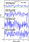 |
Fig. 1 Region with HOOH transitions toward R CrA-IRS 5A. The green line indicates the HOOH line position. Its line intensity is consistent with the rms level. All spectra have the same intensity scale, but (except for the first) are plotted with an intensity offset. |
L1544
Generally, this source reveals narrow lines that can be easily fit using a Gaussian line profile. The deconvolved spectra taken in a frequency-switching mode are shown in Fig. A.3. Assuming a temperature of 12.5 K (Tafalla et al. 1998), we determine the upper limit for the HOOH column density as 2 × 1011 cm−2.
In conclusion, our study yields a set of upper column density values for HOOH that span 2–9 × 1011 cm−2 for the investigated sources.
6 Comparison with model data
The results of the observations are summarized and compared to the predicted values by our gradient model in Table 4. The modeled water vapor results are not mentioned in this table because we do not have any observations of H2 O transitions, but the water abundances are discussed below and are compared with results from other groups. In none of the four investigated sources were we able to identify hydrogen peroxide signals, and the estimated column densities are expected to be below the derived upper limit values that roughly cover 2–9 × 1011 cm−2. These nondetections of HOOH in protostellar environments are unfortunate, but agree with a number of previous studies in which this molecule could not be detected either.
R CrA-IRS 5A (Class 1)
This source proved to be well suited for our applied gradient model. The spectra are not dominated by internal source dynamics, such as outflows, and allow a straightforward analysis. With a relative [HOOH]/[H2] abundance of 5 × 10⁻¹⁰, the model predicted an HOOH abundance nearly an order of magnitude higher than what we derived as upper limit from the observations. Geometry aspects, that is, the assumed density and temperature gradient of the YSO, are most likely not the cause for this discrepancy (Fuchs et al. 2020). Our modeled gas-phase water abundance is X = [H2O]/[H2] = 2 × 10⁻⁸ and agrees with the X ≈ 10−8 deduced by Schmalzl et al. (2014). In our model the solid HOOH abundance is indicative for the H2 O production and seems to fit to the latter number. However, the calculated gas-phase HOOH abundance is clearly too high. Although we see no fundamental contradiction between a good agreement of the model and observational values for gas-phase H2 O, the nondetection of HOOH is therefore still surprising in view of the fact that H2 O abundances (and the abundance of other molecules14) can be well described by the model.
NGC 1333-IRAS 2A (Class 0)
Because of the inner structure and dynamics, the deviation between the modeled structure of the object and the observed geometry is stronger than in the other investigated sources. To compare the observations with the model, certain assumptions (such as the restriction to the vlsr = 7.34 km s−1 component of the multipeak molecular transition lines) had to be made. Furthermore, this source is very young, which causes the model to produce unrealistically high HOOH column densities. Consequently, the predicted HOOH abundances ([HOOH]/[H2] ≈ 7 × 10⁻¹⁰–10−6) could not be confirmed and only an upper limit could be given. In case of water vapor, our model results in a relative abundance of [H2 O]/[H2] ≈3 × 10⁻⁸–6 × 10⁻⁷ depending on the age of the source, with the lower value corresponding to a more evolved source (≈ 105 yr). Observations by Kristensen et al. (2012) indicate a relative water abundance of ≈ 10−8. However, according to the same authors, the source is a young Class 0 object (~ 2 × 10⁴ yr). No conclusive result can therefore be drawn, but given the long integration times at the APEX 12 m telescope, further single-dish searches for this molecule toward IRAS 2A will most likely not result in a detection.
L1551-IRS 5 (Class 1)
Similar to NGC 1333-IRAS 2A, the spectra reveal dynamical and most likely non-LTE processes within this source. In our analysis we focused on the narrow vlsr = 7.0 km s−1 component of the lines. In our model the column density of water vapor is 3.4 × 1014 cm−2 and very close to the observed 3.1 × 1014 cm−2 by Schmalzl et al. (2014)15. Concerning the HOOH molecule, the column density of about 1 × 1013 cm−2 predicted by our model could not be confirmed by the observations. The corresponding relative [HOOH]/[H2] abundance is 3 × 10⁻⁸. The new observationally determined upper limit is about 40 times lower than this value when a temperature between 17 and 25 K is assumed. Like in the other Class 1 source, that is, R CrA-IRS 5A, the model overestimates the HOOH abundance but produces fairly good predictions for other investigated molecules.
L1544 (prestellar core)
Previous work by Tafalla et al. (1998) suggested that molecules can be seen in this source at low temperatures. In our model we assumed a 12.5 K temperature for HOOH. The upper abundance limit of this molecule is lower than the predicted value (even below the lower value given in Table 4), which is indicative of the already known weakness of the model, which tends to overestimate HOOH at early stages. The calculated relative [HOOH]/[H2] abundance is 2 × 10⁻¹²–2 × 10⁻⁹ depending on the age of the source. When the relative water vapor abundance is calculated, our gradient model results ( = 10−8–10−9) disagree with estimated abundances from observations (<1.4 × 10⁻¹⁰) by Caselli et al. (2012). Because of the low temperatures, Caselli et al. (2012) were surprised to observe water vapor emission in its inner core. Our hope that this somewhat unexpected detection might be based on mechanisms that also drive HOOH into the gas phase has not been fulfilled.
Sources in which HOOH has been searched for.
7 Discussion
So far, HOOH has been identified in only two sources, one of which (OMC-1) is still not fully verified; see Table 5. Coincidentally, these sources are the only ones in which the precursor molecule oxygen (O2) could be identified16, but with very low O2 /H2 ratios, for example, O2 /H2 ≈ 5 × 10⁻⁸ in ρ Oph A (Liseau et al. 2012).
Both sources are in regions where nearby stars cause high irradiation. New investigations of the radiation field at ρ Oph A (Lindberg et al. 2017) indicate, for example, that the H2CO rotational temperatures in the protostellar envelopes of this region are strongly enhanced close to the Herbig Be star S1 (similarly, see also the study by Lindberg et al. (2015) for the CrA star-forming region). Lindberg et al. (2017) write that “for some reason, the H2 CO gas is more prone to be heated by external radiation fields, or the H2CO abundance is enhanced in the irradiated gas, possibly due to photochemistry”. The role of an external radiation field has yet not been properly investigated for HOOH. For example, it might well be that the chemistry is changed or that desorption is enhanced. In the case of water, it is known that photodesorption takes place, but that dissociative reactions on the surface also take place, that is, the transition grain-gas can be destructive and thus decrease the water gas-phase abundance (Anderson & van Dishoeck 2008; Öberg et al. 2009).
Our model can be applied to a flat geometry and reproduces the HOOH abundance toward ρ Oph A without explicitly taking these effects into account (e.g., the desorption rate results mainly from the exothermal energy during the HOOH formation, not from radiation). This might be due to these as yet unknown or very difficult to model effects that are missing or misinterpreted in our chemical model and lead to incorrect results for the sources we investigated here. To further investigate the interplay of radiation with HOOH formation and photodesorption, we are currently bound to the two sources ρ Oph A and Orion A. However, a model refinement can only be successful if more data are available, either in the form of higher spacial resolution of the molecule distribution of HOOH and related grain-borne molecules, or as an increased set of observed molecular species to obtain a better picture of the local radiation fields17.
Evidence of HOOH in one or two sources, and the nondetection of HOOH in many investigated objects, may be interesting in connection with the chemistry of our own Solar System. Has our primordial solar environment been special? Measurements by the double-focusing mass spectrometer (DFMS) of the Rosetta Orbiter Spectrometer for Ion and Neutral Analysis (ROSINA) of the coma of comet 67P/Churyumov-Gerasimenko (Bieler et al. 2015) indicate abundant molecular oxygen and reveal an hydrogen peroxide to oxygen ratio of [H2 O2]/[O2] = (0.6 ± 0.07) × 10−3 which is very close to the ratio measured in the ρ Ophiuchi dense core [HO2]/[O2]<[H2O2]/[O2]<0.6 ⋅ 10−3 (Bergman et al. 2011a; Parise et al. 2012). Bieler et al. (2015) argued that if these gas-phase abundance ratios reflect those in the cometary ice, it would support the existence of primordial O2. Furthermore, the ρ Ophiuchi A core has been suggested to have a higher temperature, that is, about 20–30 K, compared to 10 K for most other dense interstellar clouds, which is also typical of estimates for the comet-forming conditions in the outer early solar nebula. This would suggest that our Solar System might have formed from an unusually warm molecular cloud. However, Luspay-Kuti et al. (2018) pointed out that O2 condensation in the protosolar nebula might not be the only cause of the measured abundances, but that also in situ O2 formation processes (e.g., post-accretion radiolysis) might be at play that connect this molecule with H2 O and related molecules such as hydrogen peroxide (e.g., O2 formation via HOOH dismutation or disproportionation).
8 Conclusions
At the heart of this work is the attempt to answer the question whether it can be shown that water is formed on grain surfaces through a chemical pathway that includes hydrogen peroxide as the main intermediate. For this we searched for HOOH gas-phase signatures exclusively in the dense environments of YSOs and in a prestellar core and assumed that HOOH can be released into the gas phase, thermally or through other means, after it has formed in the solid state. A model that combines a previously used chemical model (Du et al. 2012) and a physical model that takes into account the shell-like structure of typical protostellar objects was used for this purpose (see “gradient model” in Fuchs et al. 2020). Based on predictions by this model, four sources were chosen in which an HOOH detection seemed feasible and in which water has previously been detected. Despite long integration times on the APEX 12 m and IRAM 30 m telescopes, we cannot report an unambiguous hydrogen peroxide detection for any of these targets. Further support for an H2 O solid-state formation scheme through HOOH, that is, by comparing relative abundances, is therefore not possible. However, this nondetection does not exclude the proposed solid-state formation scheme. As said in the introduction, as an intermediate, HOOH may fully react to water, resulting in rather low ice and also gas-phase HOOH abundances. It is also possible that reactive desorption as a possible sublimation process is not efficient enough to build up substantial HOOH gas-phase abundances, and it is equally well possible that HOOH, after it is released from the ice, forms the starting point in a gas-phase reaction. At this stage, it is not clear how other not yet included chemical reaction mechanisms, both in the solid state and in the gas phase, will affect the abundance of HOOH. For this, follow-up studies are required. Another promising development that helps to investigate the surface-reaction scheme would be a direct solid-state detection of HOOH in the infrared region, similar to those available for H2 O ice, or other ice-borne molecules such as H2CO and CH3OH. This will not be straightforward because only a broad HOOH band around 1400–1500 cm−1 is clearly different from H2O vibrational modes. Unfortunately, vibrational modes from other abundant species can also be found in this region. Our hope is that new insights will arise from dedicated ice surveys performed by the James Webb Space Telescope (JWST) in the near future.
Acknowledgements
We thank the APEX 12 m and IRAM 30 m staff for their excellent support. We thank Peter Schilke, Thomas Möller and Álvaro Sánchez-Monge for their kind intruduction to myXCLASS.
Appendix A Tables and figures
Relevant transitions of HOOH in the (80–700 GHz) submillimeter region.
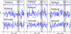 |
Fig. A.1 Frequency region with HOOH transitions (gray) toward IRAS 2A positions 1–3. All spectra have the same intensity scale, but (except for the top spectra) are plotted with an intensity offset. |
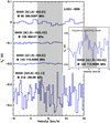 |
Fig. A.2 Frequency region with HOOH transitions (gray) toward L1551-IRS 5 using position-switching mode. All spectra have the same intensity scale, but (except for the first spectrum) are plotted with an intensity offset. The inset shows the same region around the HOOH transition 41,3 − 30,3 at 143.71263 GHz using frequency-switching mode. |
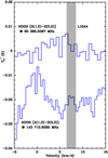 |
Fig. A.3 Frequency region with HOOH transitions (gray) toward L1544 (frequency-switching mode). Both spectra have the same intensity scale, but the lower spectrum is plotted with an intensity offset. |
References
- Ainsworth, R. E., Coughlan, C. P., Green, D. A., Scaife, A. M. M., & Ray, T. P. 2016, MNRAS, 462, 2904 [NASA ADS] [CrossRef] [Google Scholar]
- Andersson, S., & van Dishoeck, E. F. 2008, A&A, 491, 907 [NASA ADS] [CrossRef] [EDP Sciences] [Google Scholar]
- Bergman, P., Parise, B., Liseau, R., et al. 2011a, A&A, 531, L8 [NASA ADS] [CrossRef] [EDP Sciences] [Google Scholar]
- Bergman, P., Parise, B., Liseau, R., & Larsson, B. 2011b, A&A, 527, A39 [NASA ADS] [CrossRef] [EDP Sciences] [Google Scholar]
- Bieler, A., Altwegg, K., Balsiger, H., et al. 2015, Nature, 526, 678 [Google Scholar]
- Bizzocchi, L., Caselli, P., Spezzano, S., & Leonardo, E. 2014, A&A, 569, A27 [NASA ADS] [CrossRef] [EDP Sciences] [Google Scholar]
- Bottinelli, S., Ceccarelli, C., Williams, J. P., & Lefloch, B. 2007, A&A, 463, 601 [NASA ADS] [CrossRef] [EDP Sciences] [Google Scholar]
- Boudin, N., Schutte, W. A., & Greenberg, J. M. 1998, A&A, 331, 749 [NASA ADS] [Google Scholar]
- Brinch, C., Jorgensen, J. K., & Hogerheijde, M. R. 2009, A&A, 502, 199 [NASA ADS] [CrossRef] [EDP Sciences] [Google Scholar]
- Camy-Peyret, C., Flaud, J.-M., Johns, J. W. C., & Noël, M. 1992, J. Mol. Spect., 155, 84 [NASA ADS] [CrossRef] [Google Scholar]
- Carter, M., Lazareff, B., Maier, D., et al. 2012, A&A, 538, A89 [NASA ADS] [CrossRef] [EDP Sciences] [Google Scholar]
- Caselli, P., Walmsley, C. M., Zucconi, A., et al. 2002, ApJ, 565, 344 [NASA ADS] [CrossRef] [Google Scholar]
- Caselli, P., Keto, E., Bergin, E. A., et al. 2012, ApJ, 759, L37 [Google Scholar]
- Caux, E., Kahane, C., Castets, A., et al. 2011, A&A, 532, A23 [NASA ADS] [CrossRef] [EDP Sciences] [Google Scholar]
- Cazaux, S., Minissale, M., Dulieu, F., & Hocuk, S. 2016, A&A, 585, A55 [NASA ADS] [CrossRef] [EDP Sciences] [Google Scholar]
- Chen, W. P., & Graham, J. A. 1993, ApJ, 409, 319 [NASA ADS] [CrossRef] [Google Scholar]
- Chen, J.-H., Goldsmith, P. F., Viti, S., et al. 2014, ApJ, 793, 111 [NASA ADS] [CrossRef] [Google Scholar]
- Cuppen, H. M., Ioppolo, S., & Linnartz, H. 2010, Phys. Chem. Chem. Phys., 12, 12077 [NASA ADS] [CrossRef] [Google Scholar]
- Crapsi, A., Caselli, P., Walmsley, C. M., et al. 2005, ApJ, 619, 379 [Google Scholar]
- Crapsi, A., Caselli, P., Walmsley, M. C., & Tafalla, M. 2007, A&A, 470, 221 [NASA ADS] [CrossRef] [EDP Sciences] [Google Scholar]
- Du, F., Parise, B., & Bergman, P. 2012, A&A, 538, A91 [NASA ADS] [CrossRef] [EDP Sciences] [Google Scholar]
- Dulieu, F., Amiaud, L., Congiu, E., et al. 2010, A&A, 512, A30 [NASA ADS] [CrossRef] [EDP Sciences] [Google Scholar]
- Endres, C. P., Schlemmer, S., Schilke, P., et al. 2016, J. Mol. Spectr., 327, 95 [NASA ADS] [CrossRef] [Google Scholar]
- Engargiola, G., & Plambeck, R. L. 1999, The Physics and Chemistry of the Interstellar Medium, eds.: V. Ossenkopf, J. Stutzki, & G. Winnewisser (Cambridge: Cambridge University Press) [Google Scholar]
- Franklin, J., Snell, R. L., Kaufman, M. J., et al. 2008, ApJ, 674, 1015 [NASA ADS] [CrossRef] [Google Scholar]
- Fuchs, G. W., Witsch, D., Herberth, D., et al. 2020, A&A, submitted [Google Scholar]
- Goldsmith, P. F., & Langer, W. D. 1999, ApJ, 517, 209 [NASA ADS] [CrossRef] [Google Scholar]
- Goldsmith, P. F., Melnick, G. J., Bergin, E. A., et al. 2000, ApJ, 539, L123 [NASA ADS] [CrossRef] [Google Scholar]
- Goldsmith, P.F., Liseau, R., Bell, T. A., et al. 2011, ApJ, 737, 96 [Google Scholar]
- Güsten, R., Nyman, L. Å., Schilke, P., et al. 2006, A&A, 454, L13 [NASA ADS] [CrossRef] [EDP Sciences] [Google Scholar]
- Hollenbach, D., Kaufman, M. J., Bergin, E. A., & Melnick, G. J. 2009, ApJ, 690, 1497 [CrossRef] [Google Scholar]
- Hunt, R. H., Leacock, R. A., Peters, C. W., & Hecht, K. T. 1965, J. Chem. Phys., 42, 1931 [NASA ADS] [CrossRef] [Google Scholar]
- Ioppolo, S., Cuppen, H. M., Romanzin, C., et al. 2008, ApJ, 686, 1474 [NASA ADS] [CrossRef] [Google Scholar]
- Ioppolo, S., Cuppen, H. M., Romanzin, C., et al. 2010, Phys. Chem. Chem. Phys., 12, 12077 [NASA ADS] [CrossRef] [Google Scholar]
- Ivezic, Z., & Elitzur, M. 1997, MNRAS, 287, 799 [NASA ADS] [CrossRef] [Google Scholar]
- Jørgensen, J. K., Hogerheijde, M. R., van Dishoeck, E. F., et al. 2004a, A&A, 413, 993 [NASA ADS] [CrossRef] [EDP Sciences] [Google Scholar]
- Jørgensen, J. K., Hogerheijde, M. R., Blake, G.A., et al. 2004b, A&A, 415, 1021 [NASA ADS] [CrossRef] [EDP Sciences] [Google Scholar]
- Kristensen, L. E., van Dishoeck, E. F., van Kempen, T. A., et al. 2010, A&A, 516, A57 [NASA ADS] [CrossRef] [EDP Sciences] [Google Scholar]
- Kristensen, L. E., van Dishoeck, E. F., Bergin, E. A., et al. 2012, A&A, 542, A8 [NASA ADS] [CrossRef] [EDP Sciences] [Google Scholar]
- Larsson, B., & Liseau, R. 2017, A&A, 608, A133 [Google Scholar]
- Larsson, B., Liseau, R., Pagani, L., et al. 2007, A&A, 466, 999 [Google Scholar]
- Lee, J.-E., Lee, J., Lee, S., et al. 2014, ApJS, 214, 21 [NASA ADS] [CrossRef] [Google Scholar]
- Lefloch, B., Cabrit, S., Codella, C., et al. 2010, A&A, 518, L113 [NASA ADS] [CrossRef] [EDP Sciences] [Google Scholar]
- Lindberg, J. E., Jørgensen, J. K., Watanabe, Y., et al. 2015, A&A, 584, A28 [NASA ADS] [CrossRef] [EDP Sciences] [Google Scholar]
- Lindberg, J. E., Charnley, S. B., Jørgensen, J. K., et al. 2017, ApJ, 835, 3 [NASA ADS] [CrossRef] [Google Scholar]
- Liseau, R., & Larsson, B. 2015, A&A, 583, A53 [NASA ADS] [CrossRef] [EDP Sciences] [Google Scholar]
- Liseau, R., Goldsmith, P. F., Larsson, B., et al. 2012, A&A, 541, A73 [NASA ADS] [CrossRef] [EDP Sciences] [Google Scholar]
- Luspay-Kuti, A., Mousis, O., Lunine, J. I., et al. 2018, Space Sci. Rev., 214, 115 [NASA ADS] [CrossRef] [Google Scholar]
- McMullin, J. P., Waters, B., Schiebel, D., et al. 2007, ASP Conf. Ser., 376, 127 [Google Scholar]
- Melnick, G. J., & Bergin, E. A. 2005, Adv. Space Res., 36, 1027 [NASA ADS] [CrossRef] [Google Scholar]
- Miyauchi, N., Hidaka, H., Chigai, T., et al. 2008, Chem. Phys. Lett., 456, 27 [NASA ADS] [CrossRef] [Google Scholar]
- Mottram, J. C., Kristensen, L. E., van Dishoeck, E. F., et al. 2014, A&A, 572, A21 [NASA ADS] [CrossRef] [EDP Sciences] [Google Scholar]
- Minissale, M., Dulieu, F., Cazaux, S., & Hocuk, S. 2016, A&A, 585, A24 [NASA ADS] [CrossRef] [EDP Sciences] [Google Scholar]
- Möller, T., Endres, C., & Schilke, P. 2017, A&A, 598, A7 [NASA ADS] [CrossRef] [EDP Sciences] [Google Scholar]
- Nisini, B., Antoniucci, S., Giannini, T., & Lorenzetti, D. 2005, A&A, 429, 543 [NASA ADS] [CrossRef] [EDP Sciences] [Google Scholar]
- Nutter, D. J., Ward-Thompson, D., & Andre, P. 2005, MNRAS, 357, 975 [NASA ADS] [CrossRef] [Google Scholar]
- Oba, Y., Miyauchi, N., Hidaka, H., et al. 2009, ApJ, 701, 464 [NASA ADS] [CrossRef] [Google Scholar]
- Öberg, K. I., Linnartz, H., Visser, R., & van Dishoeck, E. F. 2009, ApJ, 693, 1209 [NASA ADS] [CrossRef] [Google Scholar]
- Osorio, M., D’Alessio, P., Muzerolle, J., et al. 2003, ApJ, 586, 1148 [NASA ADS] [CrossRef] [Google Scholar]
- Parise, B., Bergman, P., & Du, F. 2012, A&A, 541, L11 [NASA ADS] [CrossRef] [EDP Sciences] [Google Scholar]
- Parise, B., Bergman P., & Menten, K. 2014, Faraday Discuss., 168, 349 [NASA ADS] [CrossRef] [Google Scholar]
- Peterson, D. E., Caratti o Garatti, A., Bourke, T. L., et al. 2011, ApJS, 194, 43 [NASA ADS] [CrossRef] [Google Scholar]
- Petkie, D. T., Goyette, T. M., Holton, J. J., et al. 1995, J. Mol. Spect., 171, 145 [NASA ADS] [CrossRef] [Google Scholar]
- Pickett, H. M., Poynter, R. L., Cohen, E. A., et al. 1998, J. Quant. Spectr. Rad. Transf., 60, 883-890 [NASA ADS] [CrossRef] [Google Scholar]
- Romanzin, C., Ioppolo, S., Cuppen, H. M., et al. 2011, J. Chem. Phys., 134, 084504 [NASA ADS] [CrossRef] [Google Scholar]
- Sandell, G., Knee, L. B. G., Aspin, C., et al. 1994, A&A, 285, L1 [NASA ADS] [Google Scholar]
- Schmalzl, M., Visser, R., Walsh, C., et al. 2014, A&A, 572, A81 [NASA ADS] [CrossRef] [EDP Sciences] [Google Scholar]
- Schöier, F. L., Jørgensen, J. K., van Dishoeck, E. F., & Blake, G. A. 2002, A&A, 390, 1001 [NASA ADS] [CrossRef] [EDP Sciences] [Google Scholar]
- Shirley, Y. L., Evans II, N. J., Rawlings, J. M. C., & Gregersen, E. M. 2000, ApJS, 131, 249 [NASA ADS] [CrossRef] [Google Scholar]
- Smith, R. G., Charnley, S. B., Pendleton, Y. J., et al. 2011, ApJ, 743, 131 [NASA ADS] [CrossRef] [Google Scholar]
- Stahler, S. W., & Palla, F. 2005, The Formation of Stars (Weinheim, Germany: Wiley-VCH) [Google Scholar]
- Tafalla, M., Mardones, D., Myers, P. C., et al. 1998, ApJ, 504, 900 [NASA ADS] [CrossRef] [Google Scholar]
- Taylor, K. N. R., & Storey, J. W. V. 1984, MNRAS, 209, 5 [Google Scholar]
- Tielens, A. G. G. M. 2000, ESA SP, 577, 245 [NASA ADS] [Google Scholar]
- Van den bussche, B., Ehrenfreund, P., Boogert, A. C. A., et al. 1999, A&A, 346, L57 [NASA ADS] [Google Scholar]
- van Dishoeck, E. F., Kristensen, L. E., Benz, A. O., et al. 2011, PASP, 123, 138 [NASA ADS] [CrossRef] [Google Scholar]
- van Dishoeck, E. F., Herbst, E., & Neufeld, D. A. 2013, Chem. Rev., 113, 9043 [NASA ADS] [CrossRef] [PubMed] [Google Scholar]
- Velilla Prieto, L., Sánchez Contreras, C., Cernicharo, J., et al. 2017, A&A, 597, A25 [NASA ADS] [CrossRef] [EDP Sciences] [Google Scholar]
- Villa, A. M., Trinidad, M. A., de la Fuente, E., & Rodriguez-Esnard, T. 2017, Rev. Mex. Astron. Astrofis., 53, 525 [NASA ADS] [Google Scholar]
- Ward-Thompson, D., Buckley, H. D., Greaves, J. S., et al. 1996, MNRAS, 281, L53 [NASA ADS] [CrossRef] [Google Scholar]
- White, G. J., Liseau, R., Men’shchikov, A. B., et al. 2000, A&A, 364, 741 [NASA ADS] [Google Scholar]
- Wilkin, F. P., Chen, H.-R., Chernin, L. M., & Plambeck, R. L. 2002, ArXiv e-prints [arXiv:astro-ph/0212247] [Google Scholar]
- Wirström, E. S., Charnley, S. B., Cordiner, M. A., & Ceccarelli, C. 2016, ApJ, 830, 102 [NASA ADS] [CrossRef] [Google Scholar]
- Yıldız, U. A., Acharyya, K., Goldsmith, P. F., et al. 2013, A&A, 558, A58 [NASA ADS] [CrossRef] [EDP Sciences] [Google Scholar]
APEX 12 m project E-096.C-0780A-2015.
IRAM 30 m project ID: 097-15, run 003-16.
See “IRAM 30-meter Telescope Observing Capabilities and Organisation” by Carsten Kramer from July 22, 2016; http://www.iram.fr/GENERAL/calls/w16/30mCapabilities.pdf
GILDAS is a software provided and maintained by the Institute de Radioastronomie Millimétrique (IRAM), see http://www.iram.fr/IRAMFR/GILDAS
Using the CLASS software within the GILDAS package.
The telescope antenna parameters are taken from http://www.apex-telescope.org/telescope/efficiency/(values adapted from Güsten et al. 2006) for the APEX 12 m telescope and https:// www.iram.es/IRAMES/mainWiki/Iram30mEfficiencies (values from 26 August 2013 given in the “Improvement of the IRAM 30 m telescope beam pattern” report by Carsten Kramer, Juan Pẽnalver, and Albert Greve, Version 8.2) for the IRAM 30 m.
Python Software Foundation, https://www.python.org/
CLASS can separate between several emitting regions (core layers) with different excitations temperatures, velocity offsets, etc. However, we only used one core layer to analyze the data.
The spectroscopic data of HOOH are based on Petkie et al. (1995) and Camy-Peyret et al. (1992).
Sμ2 can be calculated by converting the intensity I
[nm2MHz] at a given temperature T
using 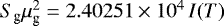
 , see Pickett et al. (1998). The partition function values Q(T) were calculated using the tables given in the CDMS and JPL catalogs.
See H2CO and CH3OH abundances in Fuchs et al. (2020).
We used a Nhydrogen column density of 1.2 × 1022 cm−2, whereas Schmalzl et al. (2014) used NH = 7.4 × 1023 cm−2, resulting in a relative H2O abundance of 4 × 10⁻¹⁰.
With the recent work by Larsson et al. (2017), more data on ρ Oph A are now available to further investigate these questions.
All Tables
Comparison between the gradient model predictions for HOOH and observational results (rotational diagram method and myXClass).
All Figures
|
Fig. 1 Region with HOOH transitions toward R CrA-IRS 5A. The green line indicates the HOOH line position. Its line intensity is consistent with the rms level. All spectra have the same intensity scale, but (except for the first) are plotted with an intensity offset. |
| In the text | |
|
Fig. A.1 Frequency region with HOOH transitions (gray) toward IRAS 2A positions 1–3. All spectra have the same intensity scale, but (except for the top spectra) are plotted with an intensity offset. |
| In the text | |
|
Fig. A.2 Frequency region with HOOH transitions (gray) toward L1551-IRS 5 using position-switching mode. All spectra have the same intensity scale, but (except for the first spectrum) are plotted with an intensity offset. The inset shows the same region around the HOOH transition 41,3 − 30,3 at 143.71263 GHz using frequency-switching mode. |
| In the text | |
|
Fig. A.3 Frequency region with HOOH transitions (gray) toward L1544 (frequency-switching mode). Both spectra have the same intensity scale, but the lower spectrum is plotted with an intensity offset. |
| In the text | |
Current usage metrics show cumulative count of Article Views (full-text article views including HTML views, PDF and ePub downloads, according to the available data) and Abstracts Views on Vision4Press platform.
Data correspond to usage on the plateform after 2015. The current usage metrics is available 48-96 hours after online publication and is updated daily on week days.
Initial download of the metrics may take a while.