| Issue |
A&A
Volume 635, March 2020
|
|
|---|---|---|
| Article Number | A127 | |
| Number of page(s) | 9 | |
| Section | Interstellar and circumstellar matter | |
| DOI | https://doi.org/10.1051/0004-6361/201937226 | |
| Published online | 24 March 2020 | |
Radiation hydrodynamical simulations of eruptive mass loss from progenitors of Type Ibn/IIn supernovae
1
Research Center for the Early Universe, Graduate School of Science, University of Tokyo, Bunkyo-ku,
Tokyo, Japan
e-mail: This email address is being protected from spambots. You need JavaScript enabled to view it.
2
Department of Astronomy, Graduate School of Science, University of Tokyo, Bunkyo-ku,
Tokyo, Japan
Received:
1
December
2019
Accepted:
10
February
2020
Abstract
Context. Observations suggest that some massive stars experience violent and eruptive mass loss associated with significant brightening that cannot be explained by hydrostatic stellar models. This event seemingly forms dense circumstellar matter (CSM). The mechanism of eruptive mass loss has not been fully explained. We focus on the fact that the timescale of nuclear burning gets shorter than the dynamical timescale of the envelope a few years before core collapse for some massive stars.
Aims. To reveal the properties of the eruptive mass loss, we investigate its relation to the energy injection at the bottom of the envelope supplied by nuclear burning taking place inside the core. In this study, we do not specify the actual mechanism for transporting energy from the site of nuclear burning to the bottom of the envelope. Instead, we parameterize the amount of injected energy and the injection time and try to extract information on these parameters from comparisons with observations.
Methods. We carried out 1D radiation hydrodynamical simulations for progenitors of red, yellow, and blue supergiants, and Wolf–Rayet stars. We calculated the evolution of the progenitors with a public stellar evolution code.
Results. We obtain the light curve associated with the eruption, the amount of ejected mass, and the CSM distribution at the time of core-collapse.
Conclusions. The energy injection at the bottom of the envelope of a massive star within a period shorter than the dynamical timescale of the envelope could reproduce some observed optical outbursts prior to the core-collapse and form the CSM, which can power an interaction supernova classified as Type IIn.
Key words: stars: massive / stars: mass-loss / supernovae: general
© ESO 2020
1 Introduction
Recent observations show that progenitors of Type IIn supernovae (SNe IIn) experienced a temporal brightening phase just before the emergence of the SNe (e.g., Elias-Rosa et al. 2018). These kinds of pre-supernova activities indicate that massive stars sometimes experience violent mass loss in the late phase of evolution and form dense circumstellar matter (CSM) as indicated for SN 1994W by Chugai et al. (2004). Kiewe et al. (2012) estimate the mass loss rates of progenitors of SNe IIn at 0.026−0.12 M⊙ yr−1 by using the relation between luminosity and mass loss rate described in Chugai & Danziger (1994). These high values cannot be explained by the standard steady mass loss model (e.g., Vink et al. 2001). In this sense, the high mass loss rate is likely to be a result of eruptive and episodic burst events.
When a core-collapse supernova (SN) takes place in a dense CSM environment formed by eruptive mass loss, the kinetic energy in the ejecta dissipated due to collision between the CSM and SN ejecta becomes the main energy source (see Chugai 1997; Smith 2017) instead of the gamma-rays emitted by radioactive decays of 56Ni. Spectra of these SNe show narrow emission lines from the CSM expanding at much slower velocities than the ejecta. Depending on whether the CSM is Hydrogen-rich or Helium-rich, these SNe are classified as SNe IIn or SNe Ibn, respectively. Since the ejecta have much more energy than the gamma-rays, these SNe IIn are brighter than other SNe II-P that are not embeded in such dense CSM.
The trigger and mechanism of the eruptive mass loss from an SN progenitor have not been fully explained though possible mechanisms of the trigger of eruption have been proposed. Quataert & Shiode (2012) and Shiode & Quataert (2014) propose that strong convection in the core during the late stage of stellar evolution excites gravity waves and these waves transport energy towards the stellar envelope and invoke mass loss. Moriya (2014) proposes that the neutrino emission in massive star takes away mass from the core and weakens the gravity, which leads to extreme mass loss. Soker & Gilkis (2017) speculate that convection coupled with stellar rotation can trigger magnetic activity and deposit energy into the outer envelope. Woosley et al. (2007) suggest that pulsational pair instability can explain explosive mass loss. Smith & Arnett (2014) deduce that treatment of turbulent convection in stellar simulation is a key factor in reproducing eruption. The results of 3D simulations by their group suggest that the merging of burning shells leads to a violent change of the energy generation rate (Mocák et al. 2018; Yadav et al. 2020). One of the key points in all of these mechanisms is the short timescale of nuclear burning in the late stage of massive star evolution as shown in Fig. 1. If the stellar envelope cannot adjust to disturbances caused by fluctuation of burning, it can no longer be in hydrostatic equilibrium.
In contrast to these scenarios, which do not require a companion star, some research suggests that the violent mass losses involve a binary system. Smith (2011) considers that the mass ejection triggered by a binary star collision. Mcley & Soker (2014); Danieli & Soker (2019) propose that the extended envelope is accreted to a companion star and releases a lot of energy and invoke mass loss. In this paper, we focus on the mass loss mechanism for a single star.
In addition to searching for the trigger mechanism of eruptive mass loss, it is also important to investigate how the outer region responds and which observational features emerge when the energy is transported to the stellar envelope by such mechanisms. This problem can be investigated through hydrodynamical simulations of the stellar envelope into which additional energy is injected. Smith (2014) classifies eruptive mass loss into two classes, namely, super-Eddington winds (Quataert et al. 2016; Fuller & Ro 2018; Ouchi & Maeda 2019) and non-terminal explosions (Dessart et al. 2010; Owocki et al. 2019). These classes seem to correspond to continuous and instantaneous extra energy injection, respectively. However, for the non-terminal explosion case, the detailed CSM distribution at the time when an SN occurs, which is important to the discussion of the CSM and SN ejecta interaction in an SN IIn or Ibn, has not been discussed in the literature. In this paper, we carried out 1D radiation hydrodynamical simulations of the eruptive mass loss by non-terminal explosions in SNe progenitors and calculated the light curves, mass loss, and ejected CSM distribution at the time of the core collapse. We made progenitors of SNe using MESA (Paxton et al. 2011, 2013, 2015, 2018), injected energy into the outer envelopes, and calculated their time evolution. In Sect. 2, we introduce the method of making progenitors by MESA and the radiation hydrodynamics code used in this paper. In Sect. 3, we present results of our calculations. We present our discussion and conclusions in Sects. 4 and 5. We should consider the mechanism of eruptive mass loss from the viewpoints of both stellar evolution theory and observations of CSM-interacting SNe. Connecting these two viewpoints is the purpose of this work.
Properties of SNe progenitors.
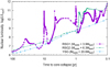 |
Fig. 1 Time evolution of nuclear burning luminosity excluding neutrino emission for each model. Details about each model are given in Sect. 2.1. A more massive star has a shorter timescale of burning, and therefore each burning stage starts at the moment closer to the time of core collapse. In this figure, RSG1 and RSG2 experience a sudden increase of nuclear burning luminosity because of the beginning of the core neon burning at about ten and 0.8 yr before core collapse, respectively. On the other hand, for model YSG, central carbon burning still continues at 0.1 yr before core collapse. |
2 Set up and methods
2.1 Progenitor models
Using a 1D stellar evolution code MESA, we made six progenitor models, named RSG1, RSG2, BSG, YSG, WR1, and WR2. Here RSG indicates red supergiant, BSG blue supergiant, YSG yellow supergiant, and WR (Wolf–Rayet). These models are used as the initial data for our 1D radiative hydrodynamical simulations. Basic parameters of these progenitors are listed in Table 1 and the density distributions are shown in Fig. 2. In their stellar evolution, these models experienced usual steady mass loss which is different from eruptive mass loss in this work and, thus, models WR1 and WR2 had already lost their Hydrogen-rich envelopes during the preceding evolution, and are expected to become Type Ibn SNe. The other models are expected to be observed as Type IIn SNe.
For RSG1, RSG2, and BSG, we chose the neon burning stage as the progenitor models because neon burning can release energy at a very high rate and is likely to cause eruptive mass loss. This burning stage occurs about ten years (RSG1), 0.8 yr (RSG2), and eight years (BSG) before the core collapse in each model. On the other hand, for YSG, WR1, and WR2, neon burning occurs only a few days before the core collapse because of their massive cores (see Fig. 1). This short timescale would prevent the ejecta of the eruptive mass loss from extending into the circum-stellar space before the core collapse. Thus, it would be impossible to reproduce the duration of the observed CSM interaction. Instead, we adopted the late stage of carbon burning for YSG, WR1 and WR2, which prolong the time to core collapse to about ten years, 0.5 yr, and 15 days, respectively. Detailed methods and the code used in MESA calculations are described in Aappendix A.
2.2 1D Radiation hydrodynamical simulation
We investigated eruptive mass loss driven by energy injection at the bottom of the envelope with an injection period shorter than the hydrodynamical timescale of the envelope by performing spherically symmetric radiation hydrodynamics simulations. We used the following Lagrangian hydrodynamics equations in a conservation form in our simulations.
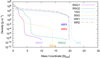 |
Fig. 2 Density distribution as a function of the enclosed mass for each progenitor listed in Table 1. |

where the mass coordinate is denoted by m, the time t, the radius r, the mass density ρ, the velocity v, the energy density E, the pressure p, and the luminosity is L. The gravity g is expressed as
 (4)
(4)
where G is the gravitational constant.
These equations were solved by the piecewise parabolic method (PPM; Colella & Woodward 1984), which uses the exact solution of the Riemann problem with initial conditions at the interface of each cell interpolated by quadratic functions. We adopted diffusion approximation with a flux limiter λ (Levermore & Pomraning 1981) to calculate the luminosity L,
 (5)
(5)
in each cell. Here a denotes the radiation constant, c the speed of light, T the temperature, and κ is the opacity. The opacity is given by
![Mathematical equation: \begin{align*} &\kappa = \kappa_{\mathrm{molecular}} + \frac{1}{\frac{1}{\kappa_{\mathrm{H}^{-1}}}+\frac{1}{\kappa_{\mathrm{e}}+\kappa_{\mathrm{Kramers}}}},\\ &\kappa_{\mathrm{molecular}} =0.1Z,\\ &\kappa_{\mathrm{H}^{-1}}= 1.1\times 10^{-25} Z^{0.5}\rho^{0.5}T^{7.7},\\ &\kappa_{\mathrm{e}}=\frac{0.2(1+X)}{\left(1+ 2.7 \times 10^{11} \frac{\rho}{T}\right) \left[1+ \left(\frac{T}{4.5\times 10^8}\right)^{0.86} \right]},\\ &\kappa_{\mathrm{Kramers}}=4\times 10^{25} (1+X)(Z+0.001)\frac{\rho}{T^{3.5}}, \end{align*}](/articles/aa/full_html/2020/03/aa37226-19/aa37226-19-eq4.png)
where κmolecular is the molecular opacity,  is the negative hydrogen opacity, κe is the electron scattering opacity, and κKramers is the Kramers opacity which includes absorption due to free-free, bound-free, and bound-bound transitions. We integrate Eq. (3) with respect to time in a partially implicit manner with a given advection term in the left hand side evaluated by the Riemann solver in each timestep (Shigeyama & Nomoto 1990). Thus, the second term on the right hand side is evaluated at the advanced time.
Essentially, we used the HELMHOLTZ equation of state (Timmes & Swesty 2000). In the region the HELMHOLTZ does not cover, we used the following equation of state:
 (11)
(11)
Accordingly, the thermal energy density u is given by
 (12)
(12)
Here R and μ are the gas constant and the mean molecular weight, respectively. The boundary conditions are given at the innermost and outermost cells as,
 (13)
(13)
We carried out four or five patterns of calculations for each progenitor, with different amounts of thermal energy injected at the bottom of the envelope (r = rinner) as shown in Table 2. Here, the envelope refers to the Helium envelope for WR1 and WR2 and the Hydrogen-rich envelope for the other models. The energy was injected at a constant rate d E∕dt as:
 (14)
(14)
for the period τ in Table 2. The value of τ is estimated from the time for the nuclear burning to generate energy that can affect the outer envelope as:
 (15)
(15)
where − Eouter is the total energy of the outer envelope, Lnuc is the total energy production rate of nuclear burning which is obtained as the output from MESA, and Einject is the total injected energy. To realize eruptive mass loss from models WR1 and WR2, we inevitably injected energy within 1 sec, which is much shorter thanτ of a few hundred years evaluated from Eq. (15) because of a large value of − Eouter. This means that an energy injection rate much larger than the nuclear luminosity is required to trigger the eruption in these two models.
As we can confirm from a comparison between Tables 1 and 2, Einject is comparable to −Eouter for every model. Thus, from Eqs. (14) and (15), we can derive d E∕d t ~ Lnuc. The energy injection rate is comparable to local peaks of the nuclear-burning luminosity of the progenitor shown in Fig. 1. For example, the nuclear-burning luminosity of RSG1 reaches a local peak of ten years before core collapse and lasts for a month, which is shorter than the dynamical timescale of the envelope. The nuclear burning around this peak releases ~ 2.5 × 1050 erg greater than Einject. Thus, these local peaks of burning luminosity prior to core collapse may be related to the dynamical eruption of the envelope. However, a considerable part of the energy from the nuclear-burning may be lost in the process of energy transport from the burning region to the bottom of the envelope, where we injected the energy Einject (see also a discussion in Sect. 4). The energy transport mechanism should be addressed in future work.
Injected energies and duration of injection.
2.3 Density distribution of homologously expanding ejecta
The pressure inside the ejecta continuously decreases due to rapid expansion since eruptive mass loss and eventually becomes unable to affect the motion of matter. We denote this epoch as t = t0. Afterwards, the motion of matter is exclusively determined by gravity. Accordingly, we quit hydrodynamical simulation described in Sect. 2.2 at t = t0 and switched to the following analytical calculation to reduce the calculation cost.
Under the assumption that only gravity force acts upon ejecta with spherical symmetry, the equation of motion is described as
 (16)
(16)
where r is the distance from the center of the progenitor, and Mr is the mass contained in a sphere of radius r. After the integration with respect to time, we obtain
 (17)
(17)
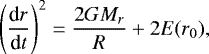
where E(r0) is the sum of the kinetic energy and the gravitational energy per unit mass for the fluid element labeled with the initial position r = r0 at t = t0. E(r0) has a positive value. This equation can be analytically solved as

where θ is a parameter, and θ = 0 corresponds to t = t0.
3 Results
As shown inTable 2, calculations were carried out for 27 different parameter sets. Because the properties of shock wave propagation and the subsequent mass eruption depend on progenitor models, we sequentially show the result for each progenitor model. It should be noted here that we could not resolve the photosphere with a reasonable number of cells for models WR1 and WR2 because of their small surface radii and therefore the information on the observable luminosity from these models is not available throughout this paper.
3.1 Model RSG1 and RSG2
In each of model, RSG1 and RSG2, an outward shock is formed immediately after the energy injection (Fig. 3), propagates toward the stellar surface and breaks out of the surface at ~ 90 days (Fig. 4). The date is measured from the moment of the energy injection. The changes in the luminosity for the first ~ 60 days are caused by inconsistent treatments of the outer optically thin layers between the MESA and our radiation hydrodynamics code. The luminosities are relaxed to the values given by the MESA models in ~60 days. After the shock breakout, the luminosity reaches the peak at around day 100. The luminosity then decreases gradually on the time scale of approximately a few ten days (Fig. 4). A larger amount of the injected energy leadsto an earlier shock emergence and a higher peak luminosity. On the other hand, the brightening timescale is not affected by the amount of the injected energy, but depends on the expansion timescale of the ejected matter, which roughly corresponds to the radius of the progenitor divided by the escape velocity. This feature remains true for the other progenitor models discussed in Sects. 3.2–3.4.
After the shock breakout and eruption, a part of the ejected matter falls back to the progenitor, while the other part acquires velocities grater than the escape velocity from the gravitational potential of the star and becomes CSM. The amount of mass loss is evaluated by the total mass of the cells with positive energy at 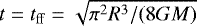 . The amount of the mass loss for this single eruption is sensitive to the amount of injected energy. A larger amount (by a factor of two) of injected energy leads to a few orders of magnitude greater amount of mass loss (Fig. 5). The CSM of an actual massive starmay be formed by recurrences of such eruption events.
Figure 6 shows the relation between the peak luminosity and the amount of mass loss. Symbols on the horizontal axis of the figure indicate the luminosities before shock arrivals. For models RSG1 and RSG2, the eruption is associated with brightening by one or two orders of magnitude, depending on the amount of the injected energy.
The CSM distribution at the time of core collapse is plotted in Fig. 7. This is one of the most important results in the present work because the distribution of the CSM directly affects the light curve of a CSM-interacting SN. A more extended profile of CSM tends to lead to an SN brightening for a longer period. The eruption in an earlier stage of stellar evolution can reproduce an extended profile because of a longer available time for the ejecta to expand with a given escape velocity. On the other hand, the nuclear burning becomes more violent in later stages as shown in Fig. 1 and more likely causeseruption. This problem is discussed in Sect. 4. We also found that the CSM formed by the eruptive mass loss has a density profile different from that of the steady wind mass loss with a constant rate Ṁ, namely ρ = Ṁ∕(4πvwindr2). In our calculation, the radius r of each fluid element in the ejecta is approximately proportional to its velocity v for every progenitor model including the other models presented in this section. This is completely different from the steady wind with a constant v = vwind. Thus, our result shows different density profiles. The outer parts of the CSM tend to have steeper slopes and the inner parts tend to have shallower slopes for every progenitor model (Fig. 8). The velocity of the CSM at the time of core collapse is another important property which determines the line-width of narrow emission line in spectra of a CSM-interacting SN, and is shown in Fig. 9. The CSM has a mean velocity determined by the escape velocity of the progenitor star (Fig. 10) and not so affected by the amount of injected energy. This means that we can estimate the property of the progenitor envelope by using the observed width of spectral lines emitted from the CSM-interacting region.
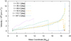 |
Fig. 3 Time evolution of the velocity profile for model RSG2 with Einj = 3.5 × 1047 erg. |
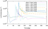 |
Fig. 4 Light curves of models RSG1 and RSG2 with different injected energies indicated by labels. |
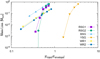 |
Fig. 5 Amount of mass loss for each model as a function of the amount of injected energy normalized with the absolute value of the binding energy of the envelope. |
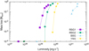 |
Fig. 6 Relation between the peak luminosity and the amount of mass loss for each model with different amounts of injected energy shown in Table 2. As mentioned at the beginning of Sect. 3, we are not able to obtain the light curve for model WR1 and WR2 and, thus, these models are absent from this figure. Symbols on the horizontal axis in this figure represent the luminosity before the arrival of outward-moving shock or diffusing photons at the photosphere. |
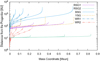 |
Fig. 7 Distribution of CSM at the time of core collapse for 27 calculations shown in Table 2. Zero of the mass coordinate corresponds to the innermost layer of the CSM ejected by eruption. |
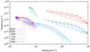 |
Fig. 8 Density profiles of CSM at the time of core collapse as functions of velocity. We used an analytical solution of Eq. (17) to derive the density profiles. |
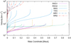 |
Fig. 9 Velocity profiles of CSM at the time of core collapse as functions of the mass coordinate. |
3.2 Model BSG
The dynamical timescale of the BSG progenitor envelope is ~ three days, much more shorter than those of RSG1 and RSG2 because of its smaller radius and higher density as shown in Table 1 and Fig. 2. This leads to a shorter propagation time of the shock (Fig. 11). The higher surface gravity requires a higher velocity of the eruption and leads to a shorter duration of brightening (Fig. 12). As in the case of RSG1 and RSG2, the peak luminosity increases with increasing injected energy and the brightening timescale is almost constant and determined exclusively by the expansion timescale of the ejecta.
Since the absolute value of the binding energy of the envelope of the BSG progenitor is about one order of magnitude larger than those of models RSG1 and RSG2 (Table 1), a shock wave in a model BSG becomes stronger and erupts more mass than the other progenitor models with a similar normalized injected energy |Einject∕Eenvelope| (Fig. 5). In addition, the eruption from models BSG is associated with a brightening by at least two orders of magnitude, which is larger than the other models (Fig. 6).
The resulting distributions of the CSM at the time of core collapse are shown in Fig. 7. Because the erupted matter expands faster than in models RSG1, RSG2, and YSG, the CSM reaches the farthest point out of the six progenitor models, although the time interval between the moments of the eruptive mass loss and the core collapse is shorter than those of RSG1 and YSG (see “Time to CC” in Table 1). SNe surrounded by CSM with these sizes are expected to have long duration light curves. The profiles of the resulting density and velocity at the time of core collapse are shown in Figs. 8–10. The mean velocity of the CSM is almost determined by the escape velocity of the progenitor star and consistent with some observed SNe IIn, such as the recent SN 2015d (Tartaglia et al. 2020).
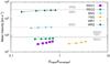 |
Fig. 10 Mean velocities of CSM ejected by eruptive mass loss event at the time of collapse as functions of the amount of injected energy normalized with the absolute value of the binding energy of the envelope. Symbols correspond to progenitor models as indicated by labels. Grey broken lines show the escape velocity of each progenitor star. |
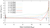 |
Fig. 11 Timeevolution of velocity profile for model BSG with Einj = 1.0 × 1049 erg. |
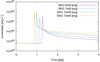 |
Fig. 12 Light curves of model BSG for injected energies specified by labels. |
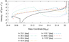 |
Fig. 13 Timeevolution of velocity profile for model YSG with Einj = 9.0 × 1046 erg. |
3.3 Model YSG
YSG progenitor model has already lost most of its Hydrogen-rich envelope by continuous mass loss during the stellar evolution calculated by MESA as shown in Table 1. The remaining Hydrogen-rich envelope (~ 0.5 M⊙) extends to R ≃ 1380 R⊙ and its density is very low ~10−9 g cc-1. Thus, this loosely bound low-density envelope shortens the life time of the shock wave because of high diffusion velocity of photons in the shocked region and slow propagation speed of the shock wave. The shock wave is already smeared out at day ~ 23.1, as shown in Fig. 13 and this leads to a gradually brightening and fading light curve (Fig. 14).
We estimate the amount of mass loss at t = 2 tff since it takes more than tff to settle the dynamics of the system. The amount of mass loss is smaller than that of any other progenitor models for the same |Einject∕Eenvelope| because of the weak shock wave (Fig. 5). The luminosity increases by a factor of ≤ 5 at the peak compared with the luminosity immediately before the shock breakout. This factor is smaller than for any other models (Fig. 6).
The CSM profile (Figs. 7–9) is similar to model RSG1 because the progenitor star has a similar escape velocity and time interval between the eruptive mass loss and the core collapse.
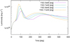 |
Fig. 14 Light curves of model YSG with different injected energies indicated by labels. |
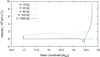 |
Fig. 15 Timeevolution of velocity profile for model WR1 with Einj = 3.0 × 1050 erg. |
3.4 Models WR1 and WR2
Progenitor models WR1 and WR2 have completely lost their Hydrogen-rich envelopes by continuous mass loss during the stellar evolution calculated by MESA and their Helium layers are exposed. For these models, the word “envelope” indicates the Helium envelope. As mentioned at the beginning of Sect. 3, we cannot obtain the information on the observable luminosity for these models.
These models have much denser envelopes than any other models, which leads to the shortest dynamical timescale ~ 200−300 s. It takes a few 100 s for the shock wave to propagate to the stellar surface (Fig. 15).
The high escape velocity is another important feature of these models (Figs. 8–10). The mean velocity of the CSM at the time of core collapse is essentially determined by the escape velocity of the progenitor star (Fig. 10) as is the case of the other models. Although the interval between the eruptive mass loss and the core collapse is only half a year for model WR1, the CSM reaches approximately a few 100 AU due to the high-velocities.
4 Discussion
We investigated the properties of eruptive mass loss from possible progenitors of SNe Ibn and IIn. Smith (2014) classifies eruptive mass loss between super-Eddington winds and non-terminal explosions. Our work is focused on non-terminal explosions (see Sect. 1) because we aim to understand recently observed short-duration outbursts prior to supernovae. The progenitor of SN 2009ip is an example of massive stars that had experienced eruptive mass loss associated with outbursts. Although the nature of 2012a and 2012b events, which are the most brightest events of SN 2009ip, is under discussion (Soker & Kashi 2013; Mauerhan et al. 2013; Pastorello et al. 2013; Smith et al. 2014; Graham et al. 2017), the progenitor had actually experienced repeated non-terminal short-duration eruptions since August 2009 (Pastorello et al. 2013). The rising timescales of such events were less than ten days. We surmise that these are shorter than the dynamical timescale of the envelope and, therefore, they must be results of shock emergence. The luminosity reached MR≈−14 at the peak and decreased over next several days. These features could be explained by hydrodynamic eruption from a blue supergiant presented in our work. However, once a progenitor experiences such an eruptive mass loss event, the remaining envelope expands and its density profile is significantly altered. Thus, if the abrupt energy injection is repeated, the feature of the eruption would be different from that of the previous eruption.
Eruptive mass loss can also be related to an “SN impostor” (Van Dyk et al. 2000). SN 1954j was found in NGC 2403 as Variable 12 (Tammann & Sandage 1968). After that its precursor star was found to have survived and the SN 1954j event is considered as an SN impostor (Van Dyk et al. 2005). Its peak luminosity MB≈−11 and brightening timescale of a few ten days could be explained by hydrodynamic eruption from a red supergiant presented in the previous section. On the other hand, some SN impostors like η Carinae’s great eruption keep their brightening phase for more than a decade. Super-Eddington winds or repeating non-terminal explosions might explain the long lasting brightening. In the latter case, we would have to consider the interaction between newly erupted ejecta and the previous one.
Next we consider the detectability of eruptive mass loss in a transient survey. Some research has succeeded in identifying the progenitors of SNe IIn by comparing the previous images of the area where the SNe emerged (e.g., Ofek et al. 2014). These researches give important clues for revealing the nature of the progenitors. On the other hand, to obtain more detailed information of progenitors, the goal is to detect eruptive mass loss event by a transient survey and to carry out the follow-up observation, as in the case of SN 2009ip. As shown in Figs. 4, 12, and 14, the luminosity from an eruptive mass loss event is expected to be ~ 1038−1040 erg s-1. Figure 16 shows the limiting bolometric luminosity for each depth of transient survey (solid lines) and the number of detected SNe IIn as a function of luminosity distance (light blue bars). An euptive mass loss event with Lbol ~ 1040 erg s-1 within 30 Mpc could be detected given a limiting magnitude of mbol = 21, while most SNe IIn have been discovered at >30 Mpc. We can expect to detect only several events per year. Moreover, to capture eruptive mass loss events from blue supergiants, a high-cadence survey with an interval of an hour or less is required.
In this work, we injected the extra energy shown in Table 2 into the bottom of the progenitor envelope without specifying the mechanism of energy transport to the envelope. We cannot identify the energy source, however, we have shown that the amount of energy generated from nuclear burning is sufficient to cause eruptive mass loss from massive stars except for Wolf–Rayet stars. Revealing the physical processes involved is one of our future aims. The results presented in this paper provide us with some clues about how this might be achieved. We obtained the relationship between extra energy injection into the stellar envelope and the amount of mass loss (Sect. 3). If the extra energy is generated from the core burning or shell burning region and transported into the envelope, some energy could be lost in the process of the energy transport. Because the diffusion timescale of photons in the stellar interior is too long, possible candidates for the energy transport mechanism are convection, gravity wave, sound wave, sub-sonic wind, and shock wave. The latter two mechanisms need to lift matter from the deep gravitational potential well. This requires an energy of ~ GṀ∕rcore, which is comparable to the energy supplied from the nuclear burning. The other mechanisms avoid the work done against the gravitational potential. It is, however, uncertain whether it can transport enough energy to trigger hydrodynamical eruption.
To reproduce the extent of the CSM around the progenitor star inferred from observations, the eruptive mass loss should have occurred a few or a few tens of years before the core-collapse. If the mass loss occurs just before the core-collapse, there is not enough timeto form such extended CSM. On the other hand, if the extra energy source for eruption originates from violent nuclear burning such as oxygen and neon burning, massive stars tend to be unable to release enough energy to cause eruptive mass loss until just before the core collapse (Fig. 1). Therefore there should be a maximum mass of the progenitor of CSM interacting-SNe. On the other hand, if the extra energy source originates from pulsational pair instability (Woosley et al. 2007), the progenitor mass on the main sequence should be higher than ~ 70 M⊙ (Woosley 2017).
While we carried out 1D simulations under the assumption of spherically symmetric mass loss, the real situation is more complex. For example, a disklike or ringlike morphology of the CSM was suggested from results of optical spectropolarimetry for SN 1998S (Leonard et al. 2000). We should carry out 2D and 3D simulations in a future work to verify if an eruptive mass loss from a rotating star or a star in a binary system can form the CSM with such a morphology implied by the observation.
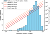 |
Fig. 16 Number of discovered SNe IIn from 2010 to 2018 in each bin of luminosity distance (Light blue bars). The data are taken from The Open Supernova Catalog (https://sne.space). Solid lines show the limiting bolometric luminosity for each depth of the survey. |
5 Conclusions
Here we investigate eruptive mass ejection, associated optical bursts from massive stars in the late phase of evolution, and the formation of the CSM. To reproduce occasional bursts observed prior to SNe IIn (and Ibn), extra energy that can unbound a part of the envelope is injected at the bottom of the stellar envelope within a period that is shorter than its dynamical timescale. We calculate the light curves (except for models WR1 and WR2), as well as the dynamical evolution of the envelope and ejected CSM, for six progenitor models by changing the amount of injected energy as a parameter.
We found that some of these results can reproduce observed outbursts, including eruptive mass loss prior to CSM interacting-SNe and SN impostors. On the other hands, compact and bluer model like blue supergiant or Wolf–Rayet stars show and imply an event with extremely short time scales (τ ~several 100 s for Wolf–Rayet model). It is expected that these kinds of events will be observed by future high-cadence transient surveys. We also found that the velocity of the ejected CSM is insensitive to the amount of injected energy, but is almost determined by the escape velocity of the progenitor, which indicates that the property of the progenitor could be inferred from the width of narrow emission lines observed for SNe IIn or Ibn, as in the case of steady wind mass loss. Moreover, CSM has a density profile different from that of the steady wind mass loss, with a constant rate Ṁ, namely ρ = Ṁ∕(4πvwindr2) (Fig. 8).
In this work, extra energy is injected only once and single burst is investigated, although observations indicate the consecutive multiple burst events. Once a progenitor experiences an eruptive mass loss event, its density profile is significantly altered and cannot recover by the moment of the SN explosion. Thus, when the energy injection is repeated, the feature of the eruption would be different from that of the previous one. Such multiple outbursts should be the subject of a future work.
Acknowledgement
This work is partially supported by JSPS KAKENHI grant Nos. 16H06341, 16K05287, 15H02082, MEXT, Japan.
Appendix A Making progenitor using MESA
Six progenitor models were generated using a 1D stellar evolution code MESA (Paxton et al. 2011, 2013, 2015, 2018), as the initial models in our radiation hydrodynamical simulations. We used the MESA with a release number of 10 108 for model RSG2 and 10 398 for the others. Here we present how we set the parameters and configuration files called “inlist”.
Stellar mass MZAMS at ZAMS and metallicity Z listed in Table 1 were set in the files named as initial_mass, initial_z, and Z_base. We used the following parameters for opacity and mass loss.
use_Type2_opacities =.true.
cool_wind_RGB_scheme = ’Dutch’
cool_wind_AGB_scheme = ’Dutch’
RGB_to_AGB_wind_switch = 1d-4
Dutch_scaling_factor = 0.8d0
Two parameters for overshooting were changed during the main sequence of model RSG1 as follows to enhance the growth of the Helium core.
overshoot_f_above_burn_h_core = 0.035d0
overshoot_f0_above_burn_h_core = 0.005d0
After the main sequence, we set a parameter as follows to ensure convergence.
dX_nuc_drop_min_X_limit = 1d-3
In models YSG, WR1, and WR2, we boosted mass loss because the normal wind scheme in MESA was insufficient to remove the Hydrogen-rich envelope. In model YSG, we changed the following parameters from the default values. In particular, the value of mixing_length_alpha was increased to ensure convergence.
remove_H_wind_mdot = 0.05d0
remove_H_wind_H_mass_limit = 0.7d0
mixing_length_alpha = 4d0
These parameters are changed to the default values once the mass of the envelope reduces to the required value. In models WR1 and WR2, the following parameters were used to remove the entire Hydrogen-rich envelope. mixing_length_alpha and varcontrol_target were changed to ensure convergence.
remove_H_wind_mdot = 0.05d0
mixing_length_alpha = 4d0
varcontrol_target = 1d-3
When the entire Hydrogen-rich envelope was removed, remove_H_wind_mdot was changed to 0.0001d0 and after a short numerical relaxation, remove_H_wind_mdot was set to zero.
The default values were used for the other parameters.
References
- Chugai, N. N. 1997, Ap&SS, 252, 225 [NASA ADS] [CrossRef] [Google Scholar]
- Chugai, N. N., & Danziger, I. J. 1994, MNRAS, 268, 173 [NASA ADS] [Google Scholar]
- Chugai, N. N., Blinnikov, S. I., Cumming, R. J., et al. 2004, MNRAS, 352, 1213 [NASA ADS] [CrossRef] [Google Scholar]
- Colella, P., & Woodward, P. R. 1984, J. Comput. Phys., 54, 174 [NASA ADS] [CrossRef] [MathSciNet] [Google Scholar]
- Danieli, B., & Soker, N. 2019, MNRAS, 482, 2277 [NASA ADS] [CrossRef] [Google Scholar]
- Dessart, L., Livne, E., & Waldman, R. 2010, MNRAS, 405, 2113 [NASA ADS] [Google Scholar]
- Elias-Rosa, N., Van Dyk, S. D., Benetti, S., et al. 2018, ApJ, 860, 68 [NASA ADS] [CrossRef] [Google Scholar]
- Fuller, J., & Ro, S. 2018, MNRAS, 476, 1853 [NASA ADS] [CrossRef] [Google Scholar]
- Graham, M. L., Bigley, A., Mauerhan, J. C., et al. 2017, MNRAS, 469, 1559 [NASA ADS] [CrossRef] [Google Scholar]
- Kiewe, M., Gal-Yam, A., Arcavi, I., et al. 2012, ApJ, 744, 10 [NASA ADS] [CrossRef] [Google Scholar]
- Leonard, D. C., Filippenko, A. V., Barth, A. J., & Matheson, T. 2000, ApJ, 536, 239 [NASA ADS] [CrossRef] [Google Scholar]
- Levermore, C. D., & Pomraning, G. C. 1981, ApJ, 248, 321 [NASA ADS] [CrossRef] [Google Scholar]
- Mauerhan, J. C., Smith, N., Filippenko, A. V., et al. 2013, MNRAS, 430, 1801 [NASA ADS] [CrossRef] [Google Scholar]
- Mcley, L., & Soker, N. 2014, MNRAS, 445, 2492 [NASA ADS] [CrossRef] [Google Scholar]
- Mocák, M., Meakin, C., Campbell, S. W., & Arnett, W. D. 2018, MNRAS, 481, 2918 [NASA ADS] [CrossRef] [Google Scholar]
- Moriya, T. J. 2014, A&A, 564, A83 [NASA ADS] [CrossRef] [EDP Sciences] [Google Scholar]
- Ofek, E. O., Sullivan, M., Shaviv, N. J., et al. 2014, ApJ, 789, 104 [NASA ADS] [CrossRef] [Google Scholar]
- Ouchi, R., & Maeda, K. 2019, ApJ, 877, 92 [NASA ADS] [CrossRef] [Google Scholar]
- Owocki, S. P., Hirai, R., Podsiadlowski, P., & Schneider, F. R. N. 2019, MNRAS, 485, 988 [NASA ADS] [CrossRef] [Google Scholar]
- Pastorello, A., Cappellaro, E., Inserra, C., et al. 2013, ApJ, 767, 1 [NASA ADS] [CrossRef] [Google Scholar]
- Paxton, B., Bildsten, L., Dotter, A., et al. 2011, ApJS, 192, 3 [Google Scholar]
- Paxton, B., Cantiello, M., Arras, P., et al. 2013, ApJS, 208, 4 [NASA ADS] [CrossRef] [Google Scholar]
- Paxton, B., Marchant, P., Schwab, J., et al. 2015, ApJS, 220, 15 [Google Scholar]
- Paxton, B., Schwab, J., Bauer, E. B., et al. 2018, ApJS, 234, 34 [NASA ADS] [CrossRef] [EDP Sciences] [Google Scholar]
- Quataert, E., & Shiode, J. 2012, MNRAS, 423, L92 [NASA ADS] [CrossRef] [Google Scholar]
- Quataert, E., Fernández, R., Kasen, D., Klion, H., & Paxton, B. 2016, MNRAS, 458, 1214 [NASA ADS] [CrossRef] [Google Scholar]
- Shigeyama, T., & Nomoto, K. 1990, ApJ, 360, 242 [NASA ADS] [CrossRef] [Google Scholar]
- Shiode, J. H., & Quataert, E. 2014, ApJ, 780, 96 [NASA ADS] [CrossRef] [Google Scholar]
- Smith, N. 2011, MNRAS, 415, 2020 [NASA ADS] [CrossRef] [Google Scholar]
- Smith, N. 2014, ARA&A, 52, 487 [NASA ADS] [CrossRef] [MathSciNet] [Google Scholar]
- Smith, N. 2017, Handbook of Supernovae, eds. A. W. Alsabti & P. Murdin (Berlin: Springer), 403 [CrossRef] [Google Scholar]
- Smith, N., & Arnett, W. D. 2014, ApJ, 785, 82 [NASA ADS] [CrossRef] [Google Scholar]
- Smith, N., Mauerhan, J., & Prieto, J. 2014, AAS Meeting Abstracts, 223, 354.30 [Google Scholar]
- Soker, N., & Gilkis, A. 2017, MNRAS, 464, 3249 [NASA ADS] [CrossRef] [Google Scholar]
- Soker, N., & Kashi, A. 2013, ApJ, 764, L6 [NASA ADS] [CrossRef] [Google Scholar]
- Tammann, G. A., & Sandage, A. 1968, ApJ, 151, 825 [NASA ADS] [CrossRef] [Google Scholar]
- Tartaglia, L., Pastorello, A., Sollerman, J., et al. 2020, A&A, 635, A39 [NASA ADS] [CrossRef] [EDP Sciences] [Google Scholar]
- Timmes, F. X. & Swesty, F. D. 2000, ApJS, 126, 501 [NASA ADS] [CrossRef] [Google Scholar]
- Van Dyk, S. D., Peng, C. Y., King, J. Y., et al. 2000, PASP, 112, 1532 [NASA ADS] [CrossRef] [Google Scholar]
- Van Dyk, S. D., Filippenko, A. V., Chornock, R., Li, W., & Challis, P. M. 2005, PASP, 117, 553 [NASA ADS] [CrossRef] [Google Scholar]
- Vink, J. S., de Koter, A., & Lamers, H. J. G. L. M. 2001, A&A, 369, 574 [NASA ADS] [CrossRef] [EDP Sciences] [Google Scholar]
- Woosley, S. E. 2017, ApJ, 836, 244 [NASA ADS] [CrossRef] [Google Scholar]
- Woosley, S. E., Blinnikov, S., & Heger, A. 2007, Nature, 450, 390 [NASA ADS] [CrossRef] [PubMed] [Google Scholar]
- Yadav, N., Müller, B., Janka, H. T., Melson, T., & Heger, A. 2020, ApJ, 890, 94 [NASA ADS] [CrossRef] [Google Scholar]
All Tables
All Figures
|
Fig. 1 Time evolution of nuclear burning luminosity excluding neutrino emission for each model. Details about each model are given in Sect. 2.1. A more massive star has a shorter timescale of burning, and therefore each burning stage starts at the moment closer to the time of core collapse. In this figure, RSG1 and RSG2 experience a sudden increase of nuclear burning luminosity because of the beginning of the core neon burning at about ten and 0.8 yr before core collapse, respectively. On the other hand, for model YSG, central carbon burning still continues at 0.1 yr before core collapse. |
| In the text | |
|
Fig. 2 Density distribution as a function of the enclosed mass for each progenitor listed in Table 1. |
| In the text | |
|
Fig. 3 Time evolution of the velocity profile for model RSG2 with Einj = 3.5 × 1047 erg. |
| In the text | |
|
Fig. 4 Light curves of models RSG1 and RSG2 with different injected energies indicated by labels. |
| In the text | |
|
Fig. 5 Amount of mass loss for each model as a function of the amount of injected energy normalized with the absolute value of the binding energy of the envelope. |
| In the text | |
|
Fig. 6 Relation between the peak luminosity and the amount of mass loss for each model with different amounts of injected energy shown in Table 2. As mentioned at the beginning of Sect. 3, we are not able to obtain the light curve for model WR1 and WR2 and, thus, these models are absent from this figure. Symbols on the horizontal axis in this figure represent the luminosity before the arrival of outward-moving shock or diffusing photons at the photosphere. |
| In the text | |
|
Fig. 7 Distribution of CSM at the time of core collapse for 27 calculations shown in Table 2. Zero of the mass coordinate corresponds to the innermost layer of the CSM ejected by eruption. |
| In the text | |
|
Fig. 8 Density profiles of CSM at the time of core collapse as functions of velocity. We used an analytical solution of Eq. (17) to derive the density profiles. |
| In the text | |
|
Fig. 9 Velocity profiles of CSM at the time of core collapse as functions of the mass coordinate. |
| In the text | |
|
Fig. 10 Mean velocities of CSM ejected by eruptive mass loss event at the time of collapse as functions of the amount of injected energy normalized with the absolute value of the binding energy of the envelope. Symbols correspond to progenitor models as indicated by labels. Grey broken lines show the escape velocity of each progenitor star. |
| In the text | |
|
Fig. 11 Timeevolution of velocity profile for model BSG with Einj = 1.0 × 1049 erg. |
| In the text | |
|
Fig. 12 Light curves of model BSG for injected energies specified by labels. |
| In the text | |
|
Fig. 13 Timeevolution of velocity profile for model YSG with Einj = 9.0 × 1046 erg. |
| In the text | |
|
Fig. 14 Light curves of model YSG with different injected energies indicated by labels. |
| In the text | |
|
Fig. 15 Timeevolution of velocity profile for model WR1 with Einj = 3.0 × 1050 erg. |
| In the text | |
|
Fig. 16 Number of discovered SNe IIn from 2010 to 2018 in each bin of luminosity distance (Light blue bars). The data are taken from The Open Supernova Catalog (https://sne.space). Solid lines show the limiting bolometric luminosity for each depth of the survey. |
| In the text | |
Current usage metrics show cumulative count of Article Views (full-text article views including HTML views, PDF and ePub downloads, according to the available data) and Abstracts Views on Vision4Press platform.
Data correspond to usage on the plateform after 2015. The current usage metrics is available 48-96 hours after online publication and is updated daily on week days.
Initial download of the metrics may take a while.