Formation channels of slowly rotating early-type galaxies

Davor Krajnović; Ugur Ural; Harald Kuntschner; Paul Goudfrooij; Michael Wolfe; Michele Cappellari; Roger Davies; Tim P. de Zeeuw; Pierre-Alain Duc; Eric Emsellem; Arna Karick; Richard M. McDermid; Simona Mei; Thorsten Naab

doi:10.1051/0004-6361/201937040

Home

All issues

Volume 635 (March 2020)

A&A, 635 (2020) A129

Full HTML

Free Access

Issue		A&A Volume 635, March 2020


Article Number		A129
Number of page(s)		26
Section		Extragalactic astronomy
DOI		https://doi.org/10.1051/0004-6361/201937040
Published online		19 March 2020

A&A 635, A129 (2020)

Formation channels of slowly rotating early-type galaxies^⋆^⋆⋆

Davor Krajnović¹, Ugur Ural¹, Harald Kuntschner², Paul Goudfrooij³, Michael Wolfe³, Michele Cappellari⁴, Roger Davies⁴, Tim P. de Zeeuw⁵^,6, Pierre-Alain Duc⁷, Eric Emsellem²^,8, Arna Karick⁴, Richard M. McDermid⁹, Simona Mei¹⁰^,11^,12 and Thorsten Naab¹³

¹ Leibniz-Institut für Astrophysik Potsdam (AIP), An der Sternwarte 16, 14482 Potsdam, Germany
e-mail: dkrajnovic@aip.de
² European Southern Observatory, Karl-Schwarzschild-Str. 2, 85748 Garching, Germany
³ Space Telescope Science Institute, 3700 San Martin Drive, Baltimore, MD 21218, USA
⁴ Sub-department of Astrophysics, Department of Physics, University of Oxford, Denys Wilkinson Building, Keble Road, Oxford OX1 3RH, UK
⁵ Sterrewacht Leiden, Leiden University, Postbus 9513, 2300 RA Leiden, The Netherlands
⁶ Max-Planck-Institut fur Extraterrestrische Physik, Giessenbachstraße, 85741 Garching, Germany
⁷ Observatoire Astronomique, Université de Strasbourg, CNRS, 11, Rue de l’Université, 67000 Strasbourg, France
⁸ Univ Lyon, Univ Lyon1, ENS de Lyon, CNRS, Centre de Recherche Astrophysique de Lyon UMR5574, 69230 Saint-Genis-Laval, France
⁹ Department of Physics and Astronomy, Macquarie University, North Ryde, NSW 2109, Australia
¹⁰ Université Paris Denis Diderot, Université Paris Sorbonne Cité, 75205 Paris Cedex 13, France
¹¹ LERMA, Observatoire de Paris, PSL Research University, CNRS, Sorbonne Universités, UPMC Univ. Paris 06, 75014 Paris, France
¹² Jet Propulsion Laboratory and Cahill Center for Astronomy & Astrophysics, California Institute of Technology, 4800 Oak Grove Drive, Pasadena, California 91011, USA
¹³ Max-Planck-Institut für Astrophysik, Karl-Schwarzschild-Str. 1, 85741 Garching, Germany

Received: 1 November 2019
Accepted: 17 January 2020

Abstract

We study the evidence for a diversity of formation processes in early-type galaxies by presenting the first complete volume-limited sample of slow rotators with both integral-field kinematics from the ATLAS^3D Project and high spatial resolution photometry from the Hubble Space Telescope. Analysing the nuclear surface brightness profiles of 12 newly imaged slow rotators, we classify their light profiles as core-less, and place an upper limit to the core size of about 10 pc. Considering the full magnitude and volume-limited ATLAS^3D sample, we correlate the presence or lack of cores with stellar kinematics, including the proxy for the stellar angular momentum (λ_Re) and the velocity dispersion within one half-light radius (σ_e), stellar mass, stellar age, α-element abundance, and age and metallicity gradients. More than half of the slow rotators have core-less light profiles, and they are all less massive than 10¹¹ M_⊙. Core-less slow rotators show evidence for counter-rotating flattened structures, have steeper metallicity gradients, and a larger dispersion of gradient values (Δ[Z/H]¯ = −0.42 ± 0.18) than core slow rotators (Δ[Z/H]¯ = −0.23 ± 0.07). Our results suggest that core and core-less slow rotators have different assembly processes, where the former, as previously discussed, are the relics of massive dissipation-less merging in the presence of central supermassive black holes. Formation processes of core-less slow rotators are consistent with accretion of counter-rotating gas or gas-rich mergers of special orbital configurations, which lower the final net angular momentum of stars, but support star formation. We also highlight core fast rotators as galaxies that share properties of core slow rotators (i.e. cores, ages, σ_e, and population gradients) and core-less slow rotators (i.e. kinematics, λ_Re, mass, and larger spread in population gradients). Formation processes similar to those for core-less slow rotators can be invoked to explain the assembly of core fast rotators, with the distinction that these processes form or preserve cores.

Key words: galaxies: elliptical and lenticular, cD / galaxies: evolution / galaxies: formation / galaxies: kinematics and dynamics / galaxies: structure / galaxies: stellar content

^⋆

Full Table B.1 is only available at the CDS via anonymous ftp to cdsarc.u-strasbg.fr (130.79.128.5) or via http://cdsarc.u-strasbg.fr/viz-bin/cat/J/A+A/635/A129

^⋆⋆

Based on observations with the NASA/ESA Hubble Space Telescope, obtained at the Space Telescope Science Institute, which is operated by the Association of Universities for Research in Astronomy, Inc., under NASA contract NAS5-26555. These observations are associated with program 13324.

© ESO 2020

1. Introduction

Early-type galaxies (ETGs) are typically considered to be featureless compared with spirals. Nevertheless, they have complex surface brightness profiles that cannot be reproduced with a single fixed form, but require a smooth variation (e.g. Caon et al. 1993; D’Onofrio et al. 1994; Graham et al. 1996; Trujillo et al. 2001; Ferrarese et al. 2006), as well as multiple components (e.g. Graham 2001; Kormendy et al. 2009; Laurikainen et al. 2010). Even before high spatial resolution imaging was available, the brightest and the most massive galaxies were known to have cores: regions where the surface brightness profile flattens to a profile that remains constant or slowly rises as the radius approaches zero (King & Minkowski 1966; Lauer 1985; Kormendy 1985; Nieto et al. 1991). High spatial resolution imaging of the Hubble Space Telescope (HST) brought unequivocal evidence that the nuclear regions of some ETGs have cores, but it also showed that the majority of luminous ETGs have continually rising cuspy profiles (Crane et al. 1993; Ferrarese et al. 1994; Lauer et al. 1995; Faber et al. 1997). Subsequent studies enlarged the sample of galaxies with high-resolution imaging capable of distinguishing central cores from cusps of various shapes (e.g. Rest et al. 2001; Ravindranath et al. 2001; Laine et al. 2003; Lauer et al. 2005; Ferrarese et al. 2006; Kormendy et al. 2009; Richings et al. 2011; Dullo & Graham 2012, 2013).

The classification of nuclear surface brightness profiles depends on the definition of what a core is, and on the functional form used to fit the light profiles (as can be seen from the discussions in the cited papers). We discuss these technical details further in Sect. 3. For the moment, we need to bear in mind that cores typically exist in galaxies brighter than M_V = −21. Cores in fainter galaxies are known, but are also rare (Lauer et al. 2007). Furthermore, cores have typical sizes of 20−500 pc (e.g. Lauer et al. 2007; Richings et al. 2011; Rusli et al. 2013), but even kiloparsec-scale cores are known (Postman et al. 2012; López-Cruz et al. 2014; Bonfini & Graham 2016; Dullo et al. 2017). Finally, core size positively correlates with the total luminosity, surface brightness, mass, and stellar velocity dispersion (Lauer et al. 2007; Dullo & Graham 2014): the more massive the galaxy, the more extended its core and the larger the difference between the observed brightness level in the core and the expected brightness based on the extrapolation of the large-scale profile (e.g. Graham 2004; Ferrarese et al. 2006; Kormendy et al. 2009; Kormendy & Bender 2009; Dullo & Graham 2012, 2013, 2014; Rusli et al. 2013). This is a key finding that delineates the formation of cores, and we review it in Sect. 5.1.

Stellar kinematics represents a crucial diagnostic of the internal structure of galaxies as it relates the projected structure with the intrinsic shape of galaxies (e.g. Franx et al. 1991; de Zeeuw & Franx 1991; Statler 1994a,b; Statler & Fry 1994). Furthermore, the information in the mean velocity, V, and the velocity dispersion, σ, of the line-of-sight velocity distribution (LOSVD) can be used to distinguish between the dominance of the ordered and random kinetic energy, or in terms of the tensor virial theorem (Binney & Tremaine 2008, p. 360), whether the flattening of the galaxy is due to its rotation or to anisotropy in the velocity dispersion vectors. This was pioneered by Binney (1978), who introduced the anisotropy diagram relating V/σ and the projected shape of galaxies, ϵ. However, the long-slit data that revealed the kinematic properties of ETGs (e.g. Bertola & Capaccioli 1975; Illingworth 1977; Schechter & Gunn 1979; Efstathiou et al. 1980; Davies et al. 1983; Davies & Illingworth 1983; Dressler & Sandage 1983; Jedrzejewski & Schechter 1988, 1989; Franx et al. 1989; Bender & Nieto 1990; Bender et al. 1994) are insufficient for the rigorous interpretation of the tensor virial theorem (Binney 2005).

The observations with SAURON, an integral field unit (IFU) (Bacon et al. 2001) of nearby ETGs (de Zeeuw et al. 2002; Cappellari et al. 2011a), showed that stellar velocity maps can be used to recognise discs (Krajnović et al. 2008, 2013a), and to rigorously apply the tensor virial theorem and use the V/σ − ϵ diagram to estimate the anisotropy of galaxies (Cappellari et al. 2007). Furthermore, the IFU data allow us to measure a more robust proxy, λ_Re, for the projected specific stellar angular momentum of ETGs (Emsellem et al. 2007, 2011). The regular or non-regular appearance of the velocity field of ETGs (Krajnović et al. 2011), directly related to the existence or lack of (embedded) discs, can also be related to the measured angular momentum (Emsellem et al. 2011). Emsellem et al. (2007) defined two classes of ETGs, where fast rotators have regular kinematics, while slow rotators have irregular velocity maps (Emsellem et al. 2011). The kinematic classification from IFU studies¹ has a strong resemblance to the structural classification of galaxies based on imaging, but it resolves a crucial problem of recognising stellar discs that are hidden due to (non-physical) projection effects or (physical) multiple structures (e.g. embedded in spheroids). Based on the structural classification of ETGs (based on HyperLeda, Cappellari et al. 2011a), it is easy to recognise galaxies that are misclassified (Emsellem et al. 2011), but also to associate slow rotators with bright ellipticals and fast rotators with discy ellipticals and S0 galaxies (e.g. Cappellari 2016).

Using the V/σ metric to separate fast and slowly rotatating ETGs, Faber et al. (1997) noted that essentially all core galaxies have low V/σ. Their sample was limited and selected in a heterogenous way (Lauer et al. 1995). Similar in size, the SAURON sample (de Zeeuw et al. 2002), for which the first robust stellar angular momenta were derived, had a more systematic selection, but was still only a representative sample. Emsellem et al. (2007) showed that while there is a strong trend between cores and slow rotators, there is no 1:1 relation (i.e. neither do all slow rotators have cores, nor are all cores found in slow rotators). This was also emphasised by Glass et al. (2011), while Dullo & Graham (2013) presented a sample of S0 galaxies (and therefore almost certainly fast rotators) with cores.

Lauer (2012) investigated a subset of galaxies with WFPC2 imaging from the volume- and magnitude-limited ATLAS^3D sample (Cappellari et al. 2011a), and confirmed the lack of a 1:1 relation between cores and slow rotators. He argued that slow rotators could be defined as galaxies with low angular momentum and core surface brightness profiles, imposing a limit of λ_Re < 0.25. This would resolve the issue of previous studies that highlighted core galaxies in fast rotators.

Krajnović et al. (2013b) collected all published nuclear surface brightness profiles and also analysed all unpublished archival HST imaging of the ATLAS^3D galaxies, increasing the Lauer (2012) sample from 63 to 135 galaxies, and demonstrated that the option of using λ_Re < 0.25 would also include a number of galaxies without cores into slow rotators. Furthermore, Krajnović et al. (2013b) investigated the physical differences between fast and slow rotators with cores. The study concluded that core fast rotators are morphologically, kinematically, and dynamically different from core slow rotators and argued against a classification scheme that combines these objects.

The mixing of fast and slow and core and no-core options remains a puzzle for a comprehensive picture of galaxy (or more precisely, ETG) formation. One of the problems was that only 135 of 260 ATLAS^3D galaxies have HST imaging at sufficient resolution. Crucially, one-third of the slow rotators were among those without classified nuclear surface brightness profiles (Krajnović et al. 2013b). These galaxies are all of relatively low mass (< 10¹¹ M_⊙) with indications of dynamically cold structures and exponential (i.e. low Sérsic index) photometric components (Krajnović et al. 2013a). Based also on the typical properties of core galaxies from the studies cited above, Krajnović et al. (2013b) made a case for these galaxies being core-less².

After obtaining HST imaging for all remaining slow rotators of the ATLAS^3D survey, we are now in a position to address the connection between nuclear surface brightness and stellar angular momentum, and develop a comprehensive view of the diversity of slow rotators and the implications for their formation and evolution, as well as their distinctiveness. Furthermore, in contrast to previous studies (with the exception of Kormendy et al. 2009), we also make use of the stellar population parameters that are now available for the ATLAS^3D sample (McDermid et al. 2015). As will become clear later, this information is crucial for separating the different assembly pathways among ETGs.

This paper is organised as follows. In Sect. 2 we describe the derivation of the stellar population parameters, and present the new HST observations and their reduction. Section 3 presents the nuclear surface brightness profiles, which allows us to present the first volume-limited sample of slow rotators with both IFU data and HST imaging. Section 4 updates the results of Krajnović et al. (2013b), presents global stellar population properties based on SAURON observation, and discusses the metallicity gradients in the context of nuclear light profiles. The discussion in Sect. 5 reviews theories of core formation and connects the results on the light profiles with results from the global IFU observations. It ends by discussing the different mass-assembly process of fast and slow rotators with and without cores and presents evidence for two separate channels of formation of slow rotators. The paper ends with a list of conclusions in Sect. 6.

2. Data analysis

2.1. Observations

We used two sets of observations based on spectroscopy and imaging. The first set was obtained using the integral-field spectrograph SAURON (Bacon et al. 2001) as part of the ATLAS^3D survey (Cappellari et al. 2011a) of nearby early-type galaxies. In particular, we here present and make available unpublished products of the stellar population analysis based on McDermid et al. (2015), pertaining to age, metallicity, α−element abundances, and gradients of these quantities.

The second set of data is based on new HST imaging. The ATLAS^3D galaxies that were not analysed by Krajnović et al. (2013b) lacked HST observations suitable for extracting nuclear surface brightness profiles. We selected all 12 remaining slow rotators with the aim to complete this class with space-based high-resolution imaging. The general properties of these galaxies are listed in Table 1.

Table 1.

General properties of the observed galaxies.

The HST data for this project were obtained through HST Program GO–13324. The primary pointings used the Wide Field Camera 3 (WFC3) with F475W and F814W filters, observed during one HST orbit. Next to the primary WFC3 observations, data were taken with the ACS (Ford et al. 1998) using the same two filters in coordinated parallel observations, yielding data 360″ away from the galactic nuclei. We here present and analyse only the WFC3 data.

The WFC3/F475W and WFC3/F814W data for each target galaxy were split into two dithered exposures with total exposure times of 1050 s and 1110 s, respectively. A short 35 s exposure was added in F814W to mitigate potential saturation of the galaxy nuclei.

2.2. SAURON stellar populations

We made use of stellar population parameters extracted from the SAURON (Bacon et al. 2001) data cubes obtained within the ATLAS^3D project. The extraction of stellar population parameters, including the emission-line correction and the measurement of the absorption-line strengths and star formation histories, are described in detail in McDermid et al. (2015). We associate with this paper the maps of age, metallicity ([Z/H]), and α−element abundance ([α/Fe]) for all galaxies in the ATLAS3D^3D sample. These were derived based on single stellar population (SSP) models as described in McDermid et al. (2015). Briefly, following McDermid et al. (2006) and Kuntschner et al. (2010), McDermid et al. (2015) used Schiavon (2007) models, which predict the Lick indices for a grid of various ages, metallicities, and α−elemement abundances. McDermid et al. (2015) derived the SSP parameters for SAURON data using three indices that are measured across the field of view of SAURON cubes (Hβ, Fe5015, and Mgb). The stellar population parameters are found by means of χ² fitting, where the best-fit SSP provides the closest model values to our observed indices in a grid of age, metallicity, and α−elemement abundances. Original models are oversampled using linear interpolation, while the uncertainties are included as weights in the sum. The errors of the final parameters are calculated as dispersions of all points that differ by Δχ² = 1.

We caution that the derived maps have to be interpreted as SSP-equivalent because we cannot expect that all stars within a region covered by a SAURON bin have the same age, metallicity, or abundance ratio. As Serra & Trager (2007) have shown, the SSP-equivalent age is biased towards the young populations, while the SSP-equivalent chemical compositions is dominated by the old population.

Maps of stellar ages and metallicities are pertinent to this paper, which were used to extract age and metallicity profiles. Metallicity profiles were derived in the same way as in Kuntschner et al. (2010) by averaging the values on stellar population maps along the lines of constant surface brightness. In this way, we ignored possible (and known) differences between the projected distribution (shape) of the stellar population parameters (e.g. metallicity, Kuntschner et al. 2010) and flux. Uncertainties at each radial point were derived as the standard deviation of all points at this ring after applying a 3σ clipping algorithm.

Gradients of the metallicity, Δ[Z/H], and the age, ΔAge, were obtained by performing straight line fits to the metallicity and age profiles (weighted by their errors). Following the definition in Kuntschner et al. (2010), the metallicity gradient is then defined as

$\begin{matrix} Δ [Z / H] = \frac{δ [Z / H]}{δ log R / R_{e}}, \end{matrix}$ $\begin{aligned} \Delta \mathrm{[Z/H]} = \frac{\delta \mathrm{[Z/H]}}{\delta \log R/R_{\rm e}}, \end{aligned}$ (1)

and the age gradient as

$\begin{matrix} Δ Age = \frac{δ log (Age)}{δ log R / R_{e}} \cdot \end{matrix}$ $\begin{aligned} \Delta \mathrm{Age} = \frac{\delta \log (\mathrm{Age})}{\delta \log R/R_{\rm e}}\cdot \end{aligned}$ (2)

The fits were limited to a region between 2″, and the half-light radius. The inner boundary was set to avoid seeing effects, while our data rarely reach far beyond the half-light radius. For massive slow rotators, SAURON observations do not cover the full R_e, and in these cases, the outer limit is set by the data. We were not able to extract stellar population profiles and gradients for two galaxies (NGC 4268 and PGC 170172), but these galaxies do not have HST data and therefore are not relevant for this study. Age and metallicity gradients are presented in Table B.1. Age, metallicity, and α-element abundance profiles, as well as the SAURON maps of the SSP equivalent stellar age, metallicity, and alpha-element abundances can be obtained from the ATLAS^3D Project website³.

2.3. HST image combination

The data processing was performed at the Space Telescope Science Institute (STScI). It involved dedicated wrapper scripts that use modules from the DrizzlePac software package, including AstroDrizzle and TweakReg.

First, we ran AstroDrizzle on every set of associated images (i.e. all images taken in one visit with the same filter) using the setting driz_separate = True. This created singly drizzled output images, which are the individual exposures after correction for geometric distortion using the World Coordinate System (WCS) keywords in the image header. The software package SExtractor (Bertin & Arnouts 1996) was then run on each singly drizzled image, using a signal-to-noise ratio threshold of S/N = 10. The resulting catalogues were trimmed using object size, location, and shape parameters chosen to reject most cosmic rays, detector artefacts, diffuse extended objects, and objects near the edges of the images. Using these cleaned catalogues, residual shifts and rotations between the individual singly drizzled images were then determined using TweakReg. This yielded formal alignment uncertainties below 0.1 pixel. The reference image was always taken to be the image that was observed first in the visit. The resulting shifts and rotations were then implemented in a second run of AstroDrizzle to verify the alignment.

Cosmic-ray rejection was performed within AstroDrizzle, which uses a process involving an image that contains the median values (or minimum value, see below) of each pixel in the (geometrically corrected and aligned) input images as well as its derivative (in which the value of each pixel represents the largest gradient from the value of that pixel to those of its direct neighbours; this image was used to avoid clipping bright point sources) to simulate a clean version of the final output image. For this step, we used the default cosmic-ray reduction settings in AstroDrizzle, combine_type = minmed, which use the median value unless it is higher than the minimum value by a 4σ threshold. Pixels that were saturated in the long F814W exposures were dealt with by flagging them as such in the data quality (DQ) extensions of the corresponding _flc.fits files. AstroDrizzle then effectively replaced the saturated pixels by the corresponding pixels in the short F814W exposures.

Sky subtraction was performed on each individual image prior to the final image combination, using iterative sigma clipping in the region shared by all images with a given filter. The resulting sky values were stored by AstroDrizzle in the header keyword MDRIZSKY of the individual _flt.fits or _flc.fits images; our wrapper script then calculated the average sky rate in e⁻ s⁻¹ for that filter and stored it in the header keyword MDRSKYRT of the final AstroDrizzle output file (_drz.fits or _drc.fits), which also uses e⁻ s⁻¹ units. This was done to allow the sky level to be added back in before performing surface photometry, which is needed to determine proper magnitude errors.

The final run of AstroDrizzle was then performed using the so-called inverse variance map (IVM) mode. These weight maps contain all components of noise in the images except for the Poisson noise associated with the sources on the image, and they are constructed from the flatfield reference file, the dark current reference file, and the read noise values listed in the image header. For the final image combination by AstroDrizzle, we used a Gaussian drizzling kernel, and parameters final_pixfrac = 0.90 pixel and final_scale 0.032″/pixel. These parameter values were determined after experimentation with appropriate ranges of values. The HST imaging used in this work as well as the reduced parallel fields were assigned a doi number (10.17876/data/2020_1⁴), and are made available at ATLAS^3D Project website (see footnote 3).

2.4. Extraction of surface brightness profiles.

We followed the common procedure, which starts with the extraction of the light profiles using the STSDAS IRAF task ellipse. This method, as described in Jedrzejewski (1987), is based on the harmonic analysis along ellipses, fitting for the centre of the ellipse, its ellipticity ϵ, and position angle Φ. The best-fit parameters describing the ellipse (ellipse centre, Φ, ϵ) were determined by minimising the residuals between the data and the first two moments in the harmonic expansion. The semi-major axis was logarithmically increased as the fitting progresses. The values of the ellipse parameters are susceptible to the influence of foreground stars and dust patches, which effectively distort the shape of the isophotes. Therefore we created object masks prior to fitting. The whole procedure is similar to that used in Ferrarese et al. (2006) and Krajnović et al. (2013b).

We converted the light profiles into surface brightness using the standard conversion formulae and the zero-points provided in the headers of the HST images. The light profile of one galaxy, NGC 1222, was considered too uncertain for any subsequent analysis. The reason for this is the presence of complex filamentary dust structures, extending several kiloparsec from the nucleus, mostly along the minor axis of the galaxy, and bounded by two bright complexes of young and bright stars. The stunning appearance of NGC 1222 was shown in the NASA/ESA Photo Release⁵ using the HST observations presented here. NGC 1222 is a recent merger remnant, and while it is clearly a slow rotator, it is somewhat special because it exhibits a prolate-like rotation (around the major axis). The galaxy is also rich in atomic gas, which has the same kinematic orientation as the stars and is distributed in the polar plane of the galaxy, making a clear link with the dusty central regions (Young et al. 2018). For our study, however, the most relevant is the extinction caused by the dust in the centre, which prohibits a robust extraction of the light profile. Therefore we excluded this galaxy from further analysis, but we highlight it in relevant figures.

The final step in the preparation of the surface brightness profiles was to address the influence of the HST point spread function (PSF). We used the same method as in Krajnović et al. (2013b): the single iteration of the Burger – van Cittert deconvolution (van Cittert 1931; Burger & van Cittert 1932). This method was shown to converge when |1 − A(x)| < 1, where A is the PSF (Bracewell & Roberts 1954), while Burger & van Cittert (1932) advised that a single iteration is often sufficient. For each filter we constructed WFC3 PSF images using the code Tiny Tim (Krist et al. 2011). The original HST image was convolved with this PSF image using the STSDAS IRAF task fconvolve to create a smoothed image. This smoothed image was run through the ellipse task, but now using the best-fit parameters (ellipse centre, Φ, ϵ) from the fit to the original HST image. This resulted in extraction of smoothed surface brightness profiles. We then approximated the effective profile as SB_eff = 2 × SB_orig – SB_conv, where SB_conv, SB_orig, and SB_eff are the convolved, original, and effective (deconvolved) surface brightness profiles, respectively. The errors on SB_eff were estimated as a quadrature sum of the errors returned by the ellipse task on SB_conv and SB_orig. The original and the effective profiles in F475W and F814W filters are presented in Figs. 1 and 2, but the subsequent analysis was performed on the effective profiles only. In Appendix A we show through a comparison with the Richardson-Lucy deconvolution (Richardson 1972; Lucy 1974) that the single iteration of the Burger-van Cittert deconvolution provides consistent surface brightness profiles down to the central WFC3 pixel. This means that the surface brightness profiles presented here have a spatial resolution comparable to those in the literature (and used in our previous work).

Fig. 1.

Surface brightness profiles of the first six low-mass slow rotators from the ATLAS^3D survey (ordered by name). Each galaxy is represented by two panels. The upper panel shows light profiles in F475W (light blue squares) and F814W (red circles) filters, and the smaller lower panel shows residuals from the fit. Open symbols are original (observed) light profiles, and filled symbols are effective (deconvolved) profiles used for the analysis. The sampling does not correspond to the pixels of the WFC3 camera, but it is defined by the tool for the isophote analysis. The Nuker fits to both filters are shown with solid (F475W) and dashed (F814W) lines. Two vertical dotted lines indicate the range used in the fit. The short vertical solid line indicates the location at which the γ′ slope is measured. Our images have a pixel scale of $0 \overset{″}{.} 032$ $0{{\overset{\prime\prime}{.}}}032$ . For a comparison with Richardson-Lucy deconvolution results, see Appendix A.

Fig. 2.

Surface brightness profiles of the second six low-mass slow rotators from the ATLAS^3D survey (ordered by name). Each galaxy is represented by two panels. The upper panel shows light profiles in F475W (light blue squares) and F814W (red circles) filters, and the smaller lower panel that shows residuals from the fit. Open symbols are original (observed) light profiles, and filled symbols are effective (deconvolved) profiles used for the analysis. The sampling does not correspond to the pixels of the WFC3 camera, but is defined by the tool for the isophote analysis. The Nuker fits to both filters are shown with solid (F475W) and dashed (F814W) lines. Two vertical dotted lines indicate the range used in the fit. The short vertical solid line indicates the location at which the γ′ slope is measured. Our images have a pixel scale of $0 \overset{″}{.} 032$ $0{{\overset{\prime\prime}{.}}}032$ . For a comparison with Richardson-Lucy deconvolution results, see Appendix A.

3. Nuclear surface brightness profiles

We are interested in characterising the surface brightness profiles as having or lacking a core. A core is a region interior to a certain break radius in which the surface brightness bends away from the steep outer profile to a shallower inner profile. The simplest functional form to describe such a surface brightness profile is a double power law (e.g. Lauer et al. 1992; Ferrarese et al. 1994), which has subsequently been further developed into the Nuker profile (Lauer et al. 1995; Byun et al. 1996).

An alternative parametrisation uses a combination of a power law and a Sérsic (1968) function, the so-called core-Sérsic model (Graham et al. 2003). Its main advantage is the fact that galaxy light profiles are typically well fitted with Sérsic functions, and not with power laws. A core-Sérsic model can, in principle, be expected to fit the surface brightness well across a wide range of radii (Trujillo et al. 2004; Ferrarese et al. 2006). Galaxies are, however, often made of multiple components, and as Kormendy et al. (2009) pointed out, instead of rigid analytic functions, it is necessary to use multiple (Sérsic) functions and fit the light profiles piecewise.

Our main goal here is not to precisely fit the surface brightness profiles over the full range of the HST imaging. Instead, we wish to determine which galaxies can be classified as having cores, a task for which the double power-law model is sufficient. For consistency with Krajnović et al. (2013b), which was partly based on the literature values, we use the Nuker profile. While the cores from the Nuker profile and the depleted cores from the core-Sérsic model are not the same structures, in practice, there is only a small number of galaxies that are classified differently (e.g. where the Nuker profile and the core-Sérsic model do not agree). Furthermore, it is often not clear if the differences are caused by the way the fit was made (e.g. radial extent, as the core and outer profiles are interdependent), the difference in the data used, or the treatment of the PSF. We note, however, that the values of the parameters defining the core (e.g. the break radius, see Sect. 3.1) are not the same for both parametrisations, and they should be used with care. For more information, we refer to the discussion in Kormendy et al. (2009), Dullo & Graham (2012, 2014), and Krajnović et al. (2013b).

3.1. Nuker profiles

We used a double power-law function of the following form (Lauer et al. 1995):

$\begin{matrix} I (r) = 2^{(β - γ) / α} I_{b} {(\frac{r_{b}}{r})}^{γ} {[1 + {(\frac{r}{r_{b}})}^{α}]}^{(γ - β) / α}, \end{matrix}$ $\begin{aligned} I (r) = 2^{(\beta - \gamma )/\alpha } I_{\rm b} \left(\frac{r_{\rm b}}{r}\right)^\gamma \left[ 1 + \left(\frac{r}{r_{\rm b}}\right)^{\alpha }\right]^{(\gamma - \beta )/\alpha }, \end{aligned}$ (3)

where γ is the inner cusp slope as r approaches 0. Galaxies with cores are marked with r_b, the radius at which a break in the light profiles occurs, and I_b is the brightness at the break. Whether a light profile has a core or is core-less is not parametrised by γ, but by the local (logarithmic) gradient γ′ of the luminosity profile, evaluated at the HST angular resolution limit, r′. The definition (Rest et al. 2001; Trujillo et al. 2004) of γ′ is given by

$\begin{matrix} γ^{'} \equiv - \frac{d log I}{d log r} |_{r = r^{'}} = - \frac{γ + β {(r^{'} / r_{b})}^{α}}{1 + {(r^{'} / r_{b})}^{α}}, \end{matrix}$ $\begin{aligned} \gamma ^\prime \equiv - \frac{\mathrm{d}~\log ~I}{\mathrm{d}~\log ~r} \bigg |_{r = r^\prime } = - \frac{\gamma + \beta (r^\prime /r_{\rm b})^\alpha }{1 + (r^\prime /r_{\rm b})^\alpha }, \end{aligned}$ (4)

where we adopted for r′ = 0.1″ as a measure of the HST resolution. In Appendix A we show that the deconvolution method we used can be trusted to about $0 \overset{″}{.} 04 - 0 \overset{″}{.} 05$ $0{{\overset{\prime\prime}{.}}}04{-}0{{\overset{\prime\prime}{.}}}05$ for WFC3 data. Therefore we could also have selected a smaller radius to derive γ′, for instance the resolution limit of 0.05. The main reason for not doing this is that part of the literature data based on Nuker profiles, including Krajnović et al. (2013b) with values for the rest of the ATLAS^3D galaxies, have used r′ = 0.1″. Using a smaller radius does not change our conclusion here, as we discuss in more detail below.

Following Lauer et al. (1995), core galaxies are defined to have γ′ ≤ 0.3, while power-law galaxies are defined to have profiles steeper than γ′ > 0.5. The values of 0.3 < γ′ < 0.5 are nominally denoted as intermediate (Rest et al. 2001). In practice, we considered all galaxies with γ′ > 0.3 not to have resolved cores, and we refer to them as core-less.

We also defined the cusp radius as the radius at which γ′ = 0.5 (Carollo et al. 1997),

$\begin{matrix} r_{γ} \equiv r_{b} {(\frac{0.5 - γ^{'}}{β - 0.5})}^{1 / α} \cdot \end{matrix}$ $\begin{aligned} r_\gamma \equiv r_{\rm b} \left(\frac{0.5 - \gamma ^\prime }{\beta - 0.5}\right)^{1/\alpha }\cdot \end{aligned}$ (5)

This radius is considered to be a more robust core scale radius, which reasonably approximates the core radius obtained from core-Sérsic fits (Dullo & Graham 2012). For galaxies that have γ′ ≥ 0.5, we adopt r_γ < 0.1″.

The fits to the deconvolved surface brightness profiles in both filters are shown in Figs. 1 and 2 and their parameters are presented in Table 2. The fitting was performed using a least-squares minimisation routine based on MPFIT (Markwardt 2009), an implementation of the MINPACK algorithm (Moré et al. 1980). The deconvolved profiles in both filters were fitted between the inner radius of 0.03″, and an outer radius that was chosen for each galaxy, limiting the spatial range in which Eq. (3) was used. Reasonable fits were obtained when the outer radius was generally close to 10″, although in a few cases, they were considerably smaller (e.g. 2″, for NGC 0661). This is a typical range for fits with the Nuker law (Lauer et al. 1995, 2005; Rest et al. 2001; Krajnović et al. 2013b).

Table 2.

Parameters of the Nuker fits and kinematic structure of the analysed galaxies.

In a few cases, the residual plots in Figs. 1 and 2 show significant deviations between the Nuker model and the data within the fitted region (e.g. NGC 3522, NGC 4191, PGC 028887, PGC 050395, and UGC 03960). The deviations in the inner parts (within the fitting region) arise partially because galaxy light does not follow a power-law profile. The Nuker fit therefore needs to be limited to different regions for different galaxies. In addition, some of our galaxies likely contain multiple light components that are most appropriately decomposed with Sérsic profiles. At large scales (> 2.5″), light profiles of our galaxies are well fitted by a Sérsic profile, while PGC 028887 and UGC 03960 are better fit with a double Sérsic model (Krajnović et al. 2013a). The HST data show that additional (Sérsic) components are also necessary within the central few arcseconds to reproduce the profiles well. We did not attempt a full decomposition of the radial profiles because we are only interested in the existence (or lack) of cores.

3.2. Are cores of our galaxies beyond the HST resolution limit?

Our galaxies are at distances of between 25 and 40 Mpc, and it is not obvious that even with the HST resolution we would be able to resolve or even detect their cores. Based on our choice for r′ = 0.1″ and a limiting distance of 40 Mpc, the lower limit to the size of cores that we can detect is about 19 pc, while sizes a factor of two smaller would be detectable for r′ = 0.05″. This means that we cannot expect to detect any core with a physical radius smaller than ∼10 pc. Cores detected in previous works have characteristic sizes typically larger than 20 pc (e.g. Lauer et al. 2007; Krajnović et al. 2013b; Dullo & Graham 2014).

As defined in the previous section, two relevant radii are related to the core size within the Nuker profile: r_b and r_γ. The former is the radius at which the Nuker profile has the maximum curvature, or the location of the transition between the two power laws of Eq. (3). The latter is a characterisation of the physical size of the core, defined as the location at which the logarithmic slope of the galaxy surface brightness reaches a given value of γ′, as shown in Eq. (5). The choice of γ′ is somewhat arbitrary, but as Carollo et al. (1997) and Lauer et al. (2007) showed, γ′ = 0.5 is a natural way to separate cores from core-less galaxies, and it provides tighter relations with other galaxy parameters. However, r_γ does not specify the actual size of the core, but should be considered, in the words of Lauer et al. (2007), as “just a convenient representative scale”.

Our galaxies have γ′ > 0.5 (all except NGC 4191 in F475W filter), and therefore the cusp radius is not well defined for the combination of the α and β parameters. As is the custom for such galaxies, we placed an upper limit on the core size of r_γ < 0.1″ (see Table 2 for values in parsec). Given the distances to our galaxies, this places a limit to the core scales of < 10 − 20 pc, as expected from the resolution arguments. The possibility remains that our galaxies harbour smaller cores.

Known galaxies with cores are all massive, bright, and have large velocity dispersions, therefore it might be an issue that the current scaling relations, such as r_γ − σ or the r_γ − M_V relations, are not representative of our galaxies. In order to use them for our galaxies, they need to be extrapolated to σ ∼ 100 km s⁻¹ or M_V < −20, while they are currently confined to σ > 150 and M_V > −21 (Figs. 4 and 5 in Lauer et al. 2007). When we apply these relations to estimate the sizes, the potential cores in our galaxies would have r_γ < 5 pc (for r_γ − σ) and r_γ < 10 pc (for r_γ − M_V, assuming V − K = 3 colour for our galaxies and using the absolute K-band magnitudes from Table 1). Even though r_γ < r_b, and not the physical size of the core, it is likely that we would not be able to detect such small cores. The same conclusion remains valid for most galaxies when we use assume r′ = 0.05 (and r_γ < 0.05″).

An alternative is to use relations from Dullo & Graham (2014), such as their r_b − σ or r_b − μ₀ (Fig. 5 in that paper). These relations are made for core-Sérsic fits and are based on a smaller sample than the Lauer et al. (2007) relations. They also need to be extrapolated because the velocity dispersion is limited to σ > 200 km s⁻¹, while μ₀ > 14 (V-band surface brightness). Furthermore, we recall that r_b (core-Sérsic) ≈1/2r_b (Nuker) (Dullo & Graham 2014), but r_γ ∼ r_b (core-Sérsic) (Dullo & Graham 2012). Nevertheless, using the r_b − μ₀ relation on our galaxies with typical surface brightness in F475W filter between 14 and 15 mag arcsec⁻², we might expect core sizes of 20−40 pc, parametrised as r_b (core-Sérsic), while the r_b − σ relation predicts for most of galaxies r_b < 5 pc. These values show a considerable spread in the estimated sizes, and point to a general problem of predicting the (relevant) sizes of cores: they are highly uncertain.

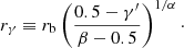
In Fig. 3 we compare the sizes of cores (r_γ) and distances to galaxies in the ATLAS^3D sample. We over-plot the effect of the resolution of the HST and the upper limits for our galaxies from Table 2. They show that our observations are able to detect cores with sizes typical for ETGs, even at the distance limit of the sample. We also show a histogram with the fraction of core-less galaxies as a function of distance. The purpose is to demonstrate that there is no sudden increase in the fraction of core-less galaxies with distance, which might be the case if we were missing cores because of the resolution effects. There is a lack of galaxies with large cores at distances beyond ∼35 Mpc, but this is a feature of the local universe and the ATLAS^3D sample, which contains no massive galaxies at these distances.

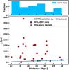Fig. 3.

Distribution of sizes (r_γ) and distances to core ATLAS^3D galaxies (red squares). The blue solid line shows the HST limit of r_γ < 0.1″, assumed for all galaxies that have γ′ > 0.5. Below this line, cores cannot formally be detected. Circles on the line are the upper limits on possible core sizes for galaxies presented here with values from Table 2. The histogram at the top shows the fraction of core-less galaxies in bins of distance. There is no evidence for an increase of the fraction of core-less galaxies as a result of resolution effects.

Table 2 shows that none of our galaxies have a core larger than 10−20 pc. They could have undetected cores from sub-parsec up to a few parsec in size, but these are obviously very different from cores in other slow rotators. As we discuss later, the galaxies presented here differ from other slow rotators, most notably in mass and stellar population parameters. It is crucial that the galaxies we investigated here are slow rotators because this information was absent from all previous samples that were used to investigate nuclear surface brightness profiles. We showed that among slow rotators are galaxies that have large cores, tens to hundreds of parsec in size (Krajnović et al. 2013b, and see also Lauer 2012), and we here address slow rotators that in the most extreme case cannot have cores larger than a few parsec.

For the rest of the paper we assume that the galaxies analysed here are all core-less. When we assume that all galaxies with non-regular kinematics have similar formation histories and that slow rotators should be core galaxies (e.g. Lauer 2012), then this is already an unexpected result.

4. Results: not all slow rotators have cores

In this section, we first update Krajnović et al. (2013b) with information on the surface brightness profiles for all ATLAS^3D slow rotators. We then extend the analysis using the information on the stellar populations, in particular the metallicity and age gradients.

4.1. Cores versus rotation

4.1.1. Global kinematic parameters

Figures 4 and 5 present the specific angular momentum (λ_Re) versus the observed elliptiticy and the velocity dispersion within one half-light radius for ATLAS^3D galaxies, respectively. The data are the same as in Figs. 4 (left) and 7 of Krajnović et al. (2013b), where we now complete the information on nuclear light profiles for all remaining slow rotators. Two results are evident. Stellar angular momentum alone remains an ambiguous predictor of the presence of cores (Fig. 4). The transition region between fast and slow rotators (0.1 < λ_Re < 0.2) contains galaxies with both types of nuclear surface brightness profiles. Only galaxies with the lowest measured values for λ_Re are more likely to have cores. Notably, core-less light profiles seem to be more likely associated with flatter slow rotators, dominating the distribution for ϵ_Re > 0.25.

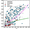Fig. 4.

Specific stellar angular momentum vs. the observed ellipticity of the ATLAS^3D galaxies. Small open circles are galaxies with no available HST observations, and small filled circles are galaxies for which the central surface brightness profile is uncertain, mostly because of a dusty nucleus. Red diamonds are core galaxies (γ′ ≤ 0.3), and blue pentagons are core-less galaxies (γ′ > 0.3). The green solid line separates fast from slow rotators following Emsellem et al. (2011), and the grey solid line is the Cappellari (2016) alternative. The dashed magenta line shows the edge-on view for spheroidal galaxies integrated up to infinity with β = 0.7 × ϵ_intr, as in Cappellari et al. (2007). Other dashed lines show the same relation projected at inclinations of 80°, 70°, 60°, 50°, 40°, 30°, 20°, and 10° (from right to left). The dotted lines show the change in location for galaxies of intrinsic ϵ_intr = 0.85, 0.75, 0.65, 0.55, 0.45, 0.35, and 0.25 (from top to bottom). This plot differs from Fig. 4 (left) of Krajnović et al. (2013b) in that all slow rotator galaxies now have nuclear surface brightness characterisation, but the number of slow rotators with cores did not increase. NGC 1222 is the small black symbol on the grey line.

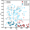Fig. 5.

Specific stellar angular momentum vs. stellar velocity dispersion within the half-light radius for the ATLAS^3D sample. Galaxies are separated into core slow rotators, core fast rotators, core-less slow rotators, and core-less fast rotators, as shown on the legend. Galaxies with uncertain profiles and galaxies with no HST data are shown with small solid and open symbols, respectively. The box delineated by solid black lines is from Fig. 7 of Krajnović et al. (2013b), where mostly cores occur. Data presented here show that outside the box there are no new core galaxies, while the one galaxy that was previously unclassified (NGC 0661, the upper blue symbol within the box) also has a core-less surface brightness profile. The galaxy with an uncertain surface brightness profile in the box is NGC 3607, while NGC 1222 is the small solid circle with σ ∼ 90 km s⁻¹ and λ_R ∼ 0.15.

On the other hand, a combination of the effective velocity dispersion, σ_e, and λ_Re, remains the best predictor of the nuclear light profile structure (Fig. 5), as noted in Krajnović et al. (2013b). All slow rotators with a velocity dispersion lower than about 160 km s⁻¹ have core-less light profiles. Within the rectangle, defined as σ_e > 160 km s⁻¹ and λ_R < 0.25, where essentially all core galaxies are found, there are now two core-less galaxies, and one with an uncertain profile. This means that only about 10% of the galaxies within the box are likely to have core-less profiles. When we restrict this to σ_e > 200 km s⁻¹ and λ_Re < 0.25, essentially all galaxies have cores. This provides an interpretation for studies of large samples, such as the one of Graham et al. (2018), who investigated the kinematics of MANGA galaxies for which high-resolution nuclear stellar profiles are not available. Assuming that our low number statistics can be taken as an indicator, about 15% of galaxies with 160 < σ_e < 200 km s⁻¹ and λ_Re < 0.25 in the MANGA sample could be core-less. Nuclear surface brightness profiles of all MANGA galaxies with σ_e > 200 km s⁻¹ and λ_Re < 0.25 most likely exhibit cores.

Galaxies in the boxed region of Fig. 5 are separated into two groups with a jump in λ_Re for about 0.05−0.1. The group of the higher λ_Re (and σ_e < 220 km s⁻¹) corresponds to the group of fast rotators with cores in Fig. 4. Slow rotators with cores are confined to the lowest values of λ_Re, but extend to the highest velocity dispersions.

Slow rotators are heterogeneous in terms of the mass (spanning almost two orders of magnitude in the ATLAS^3D sample), environment, and kinematics (Emsellem et al. 2011; Cappellari 2016). Their velocity maps exhibit no net rotation, various types of KDCs, as well as velocity maps that show rotation, but it is irregular and with twists (Krajnović et al. 2008, 2011). The velocity maps of the slow rotator sub-sample presented here are as diverse. Notably, 7 of 11 galaxies (we also excluded NGC 1222 from the kinematic analysis of the sample) have KDCs or counter-rotating cores (CRC), one galaxy is classified as a 2σ (it contains a counter-rotating disc, recognisable with two peaks in the velocity dispersion maps), with the remaining three having non-regular rotation (NRR)⁶ velocity maps. In the last column of Table 2 we copy the kinematic structure of these galaxies from Krajnović et al. (2011).

The high incidence of KDC/CRCs among core-less slow rotators is worth a closer look, especially when we consider that CRCs are a sub-class of KDCs in which the rotation of the KDC is opposite to the orientation of the main body (the angle difference is ∼180°). In Table 3 we combine the information from this work (Table 2), the surface brightness profile classification from Table C.1 of Krajnović et al. (2013b), and the kinematic structures from Table D.1 of Krajnović et al. (2011). We removed NGC 1222 from the total of 36 ATLAS^3D slow rotators, and show that only 43% of the remaining 35 slow rotators have cores. The relative fraction of KDCs or CRCs is similar between core and core-less galaxies, however, and the same is true for galaxies with NRR velocity maps. The clear difference in the kinematics is visible in the remaining two kinematic classes. Low-velocity (LV) features are almost entirely found among core slow rotators, while 2σ features are found only among core-less slow rotators.

Table 3.

Incidence of kinematic and photometric features among ATLAS^3D slow rotators.

An exception to the rule is NGC 6703, classified as LV and a core-less slow rotators, but its non-rotation arises because this galaxy is seen almost face-on, as has been suggested by Emsellem et al. (2011) and confirmed by dynamical modelling of Cappellari et al. (2013a). We also highlight the case of the core galaxy NGC 5813, the first galaxy that was recognised as having a KDC (Efstathiou et al. 1980, 1982). Recent high-quality MUSE data also showed a 2σ feature in their velocity dispersion map (Krajnović et al. 2015). This galaxy is unusual because it apparently does not have two counter rotating discs, but the MUSE data can be reproduced with a dynamical model constructed of two counter-rotating short axis tube orbital families. Strictly speaking, NGC 5813 could be included in Table 3 as the only core 2σ, but we prefer to keep it as a KDC, reserving the 2σ class for galaxies that are made of counter-rotating discs. Nevertheless, NGC 5813 is an important case because it shows that counter-rotation does not need to be solely associated with discs, but likely comes in a spectrum of possible orbital structures.

On the other hand, NGC 0661 (a CRC) and NGC 7454 (a NRR) could also be considered 2σ galaxies. For these two galaxies, Cappellari (2016, Fig. 12) constructed successful dynamical models made of two counter-rotating discs. If we assumed that NGC 0661 and NGC 7454 were such objects, the fraction of various kinematics classes of core-less slow rotators would change: f(CRC) = 0.15, f(2σ) = 0.3, and f(NRR) = 0.2, but the overall conclusions remain the same. A significant fraction of core-less slow rotators are dominated by counter-rotation, which decreases the net angular momentum.

4.1.2. Local kinematic parameters

The difference in the kinematics between core slow rotators and core-less slow rotators must originate in their formation. The statistics in Table 3 suggests that the main difference is the existence of hidden disc-like structures, which by virtue of the counter-rotation leads to a low angular momentum. To investigate this conjecture further, we also considered the higher order moments of the LOSVD, in particular, the h₃ Gauss-Hermite moment, as defined by van der Marel & Franx (1993). Figure 6 shows that core slow rotators and core-less slow rotators have marginally different distributions in the V/σ − h₃ plane: that there is an anti-correlation between V/σ and h₃ for core-less slow rotators. This anti-correlation is not strong, but the distribution of the blue contours (core-less slow rotators) is clearly skewed with respect to the symmetric distribution of red contours (core slow rotators). We quantify the difference between the distributions in Fig. 6 using

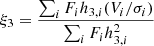
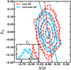$\begin{matrix} ξ_{3} = \frac{\sum_{i} F_{i} h_{3, i} (V_{i} / σ_{i})}{\sum_{i} F_{i} h_{3, i}^{2}} \end{matrix}$ $\begin{aligned} \xi _3 = \frac{\sum _i F_i h_{3,i}(V_i/\sigma _i)}{\sum _i F_i h_{3,i}^2} \end{aligned}$ (6)

Fig. 6.

Local V/σ − h₃ diagram for slow rotators separated into core (dashed red line) and core-less (solid blue line). Contours are based on logarithmic number counts starting from 0.25 and 0.5 and then increase with a step of 0.5 until 2.5 for core slow rotators and 1.5 for core-less slow rotators, respectively. Only bins with an uncertainty δh₃ < 0.05 and σ_e > 120 km s⁻¹ are plotted. Straight lines show the slope of the distributions as measured by the ξ₃ parameter (see text for details). The inset histogram shows the distribution of the ξ₃ obtained using the jackknife method, where from the original distributions for core slow rotators and core-less slow rotators one galaxy (in each sub-sample) was randomly removed, and the ξ₃ remeasured. The histograms are notably different, with core-less slow rotators having steeper slopes (ξ₃ < 1). This confirms the robustness of the weak anti-correlation between the V/σ and h₃ distributions of core-less slow rotators.

from Frigo et al. (2019), where for each spatial bin i, there is the local flux F_i, the mean velocity V_i, the velocity dispersion σ_i, and the skewness parameter h_3, i of the LOSVD. This global parameter measures the slope of the distribution of points in the h₃ − V/σ plane, as shown by straight lines in Fig. 6. It is tuned such that when h₃ and V/σ are fully (anti-)correlated, the correlation is given by h₃ = (1/ξ₃)V/σ. Frigo et al. (2019) showed examples of various h₃ and V/σ distributions with and without correlations, and corresponding ξ₃ parameters. Fast-rotating galaxies have ξ₃ < −4, while slow rotators are expected to have ξ₃ close to 0. Positive ξ₃ are also possible and often found in barred systems. In our case, as shown in Fig. 6, core-less slow rotators combined have ξ₃ = −1.3, and core slow rotators combined have ξ₃ = −0.5. The difference between the two distributions is small because all galaxies are slow rotators, but it is significant.

We tested the significance of the difference between the two distributions by randomly removing one core-less slow rotator and one core slow rotator from the distributions and remeasuring the slope of the distribution through the ξ₃ parameter. The aim was to show how the distributions of points in the h₃ − V/σ are dependent on individual galaxies, that is, whether the distributions are skewed by, for example, a single galaxy. The resulting histograms of a jackknife sequence of 100 such samples are shown in the inset panel of Fig. 6. The difference in the two ξ₃ distributions is clearly visible, where core slow rotators show a relatively narrow distribution that peaks at low ξ₃ values compared to core-less slow rotators. As expected from the original sample, the distribution of ξ₃ values for core-less slow rotators is centred on a value indicating a stronger anti-correlation between V/σ and h₃. However, the distribution is wide and it also has multiple peaks that result from large variations between individual galaxies. The small overlap between the two histograms indicates a clear difference of the orientations in the h₃ − V/σ plane, and a stronger anti-correlation between h₃ and V/σ for core-less slow rotators.

The anti-correlation between V/σ and h₃ is one of the crucial differences between galaxies with and without discs (Bender et al. 1994; Krajnović et al. 2011, 2013a; van de Sande et al. 2017). These anti-correlations are typically found in remnants of gas-rich mergers (Bendo & Barnes 2000; Jesseit et al. 2005, 2007; González-García et al. 2006; Naab et al. 2006a, 2007; Hoffman et al. 2009; Röttgers et al. 2014) or in simulations of objects that did not have a strong feedback mechanism turned on (e.g. no AGN feedback Dubois et al. 2016; Frigo et al. 2019). We therefore conclude that it is likely that core-less slow rotators originate from dissipative processes and contain embedded discs or disc-like structures.

4.2. Cores in the (M, R_e) diagram

The difference between core slow rotators and core-less slow rotators is also well illustrated in the mass – size relation. Figure 7 is an update of Fig. 6 from Krajnović et al. (2013b) and shows the mass – size relation for slow rotators (top) and fast rotators (bottom) in the ATLAS^3D sample, with masses and sizes from Cappellari et al. (2013a). Again there is a confirmation of the expectation that all low-mass ETGs (< 0.8 × 10¹¹ M_⊙) are core-less (Faber et al. 1997; Kormendy et al. 2009), but the size, the velocity dispersion, or the mass are not decisive parameters for finding cores. Mass seems to be a robust discriminator between core and core-less galaxies only for slow rotators; there are no core-less slow rotators above ∼10¹¹ M_⊙. It should be noted that ATLAS^3D does not probe galaxies more massive than 8 × 10¹¹ M_⊙, and because beyond this mass fast rotators become very rare (e.g. Veale et al. 2017), it could be that beyond some high value, the galaxy mass remains the only parameter separating core from core-less galaxies, regardless of their stellar angular momentum content. To settle this issue, more observations of most massive galaxies are required because there are BCGs that have core-less profiles (Laine et al. 2003). Their absolute magnitude is typically less bright than −23 mag in V band, which limits their mass to about 10¹² M_⊙. Nevertheless, it would be interesting to see if these galaxies are fast or slow rotators because not all central galaxies, or BCGs in particular, are found to be slow rotators (Brough et al. 2011; Jimmy et al. 2013; Oliva-Altamirano et al. 2017).

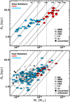Fig. 7.

Mass – size relations for ATLAS^3D fast (bottom) and slow (top) rotators. In both panels, small open symbols show galaxies with no HST imaging, and small filled symbols represent galaxies with uncertain light profiles. The colour specifies core (red) and core-less galaxies (light blue). Symbols refer to kinematic classes defined in Krajnović et al. (2011, see also Table 3), including KDC, CRC, 2σ, LV, NRR, and RR. Vertical lines are drawn at characteristic masses of 0.8 and 2 × 10¹¹ M_⊙. Constant velocity dispersions are shown by dashed lines. Compared to Fig. 6 of Krajnović et al. (2013b), the new HST data show that core galaxies do not appear in galaxies less massive than 0.8 × 10¹¹ M_⊙, and that all slow rotators more massive than 10¹¹ M_⊙ have cores. The black symbol in the top panel is NGC 1222.

Figure 7 also shows the kinematic type of galaxies. As shown before, complex kinematic features, which include KDC, CRC, LV, NRR, and 2σ, are found in slow rotators (Krajnović et al. 2011; Emsellem et al. 2011). Among slow-rotators there is a weak trend that KDC are found in more massive galaxies than CRC and 2σ features, but exceptions exist. Much more robust is the fact that core-less slow rotators overlap with (core-less) fast rotators in the mass, size, and velocity dispersion. Conversely, core slow rotators occupy a special place in the mass – size diagram, being both the most massive and the largest galaxies and having the highest velocity dispersions. They extend beyond the location of fast rotators and spiral galaxies (e.g. Cappellari et al. 2011a, 2013b) and form a progressively thin distribution clustering close to the zone of exclusion (Krajnović et al. 2018a).

The most conspicuous difference between core-less slow rotators and core slow rotators is their masses. The high-mass core slow rotators are found in dense regions, such as clusters and groups of galaxies, and they often are the central galaxies in such environments (see review by Cappellari 2016). Low-mass core-less slow rotators are found in various environments from clusters to the field (Cappellari et al. 2011b). Our sample is too small to distinguish between mass or environmental effects as the driver for the kinematic differences (e.g. Brough et al. 2017; Greene et al. 2017; Graham et al. 2019). Nevertheless, as the galaxy mass increases, core-less galaxies give way to core galaxies. According to the currently favoured core formation scenario (see Sect. 5), cold gas needs to be absent for making cores. The transition between core-less slow rotators and core slow rotators visible in the top panel of Fig. 7 therefore may be the result of a decreasing role for the nuclear cold gas in the mass assembly.

Cores also exist in fast rotators. They are rare (8% of fast rotators with HST imaging, compared e.g. to 57% of core-less slow rotators), and their hosts are kinematically different from core slow rotators (Krajnović et al. 2013b). Compared to the rest of fast rotators, core fast rotators are typically more massive, have a higher effective velocity dispersion, and a lower stellar angular momentum (e.g. Figs. 4 and 7). They occupy the same regions in the mass – size space as slow rotators with cores, except that they do not extend as high in mass and size. These galaxies are further discussed in Sect. 5.4.

4.3. Metallicity gradients: evidence for different assembly processes of core and core-less galaxies

Mass assembly can also be traced by stellar population properties. In this respect, gradients of stellar populations, in particular, their metallicity gradients, are heralded as discriminators between various formation models (White 1980). We investigate this prediction by first showing the radial metallicity profiles of all ATLAS^3D slow rotators in Fig. 8. We consider metallicity profiles in galaxies with young stellar populations as not reliable (for our sample, this means anything younger than 5 Gyr). The slow rotator with the youngest stellar populations is NGC 1222, which we exclude from this analysis and highlight in the figures. We highlight in passing also NGC 4191 and NGC 4690 because their stellar ages fall below the 5 Gyr limit at some radial bins. The luminosity-weighted stellar ages within the half-light radius for these galaxies are 6 and 4 Gyr, respectively (McDermid et al. 2015). For this reason, and because their metallicity radial profiles do not look different from the rest of the slow rotators, we kept them for further analysis.

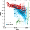Fig. 8.

Radial variation of metallicity profiles averaged along isophotes for all ATLAS^3D slow rotators and normalised by the half-light radii. Blue circles show metallicity profiles of slow rotators with core-less surface brightness profiles, and red squares show profiles of slow rotators with cores. Green circles belong to NGC 1222, which was not classified because of the dust. As seen in Fig. 7, core galaxies are more massive slow rotators, and the offset between the metallicity profiles of core and core-less galaxies is explained as the mass trend. Core galaxies are also larger than core-less galaxies, which explains the offsets along the horizontal axis between the two types of galaxies. The profiles differ also in their slopes, however.

The metallicity profiles in Fig. 8 are normalised to the effective radius of galaxies (from Cappellari et al. 2013a) to remove the size dependence. The mass trend, in which more massive core slow rotators have higher mean absolute values of the metallicity profiles, is visible in the figure. The size difference between core slow rotators and core-less slow rotators is also highlighted by the fact that in core slow rotators, which are typically larger galaxies, we probe smaller relative radii. Furthermore, there seems to be a global difference in the slope of the metallicity profiles between core slow rotators and core-less slow rotators, and we quantify this by considering metallicity gradients.

Figure 9 shows metallicity gradients for all ATLAS^3D galaxies (left-hand panel) and ATLAS^3D galaxies with HST imaging, highlighting the slow rotators (right-hand panel). In both panels we highlight core and core-less galaxies and their correlation with the fast or slow rotators. A similar figure showing a mass dependence on the metallicity gradient was also presented in Kuntschner (2015). The trend in the figure is consistent with trends in the literature when the specific sample selections are taken into account (Spolaor et al. 2009, 2010; Rawle et al. 2010; Koleva et al. 2011; La Barbera et al. 2012; Li et al. 2018a). Most ATLAS^3D galaxies have negative gradients, implying higher values in the centre, while many of the galaxies with positive gradients have younger stellar populations. Recent IFU surveys of late- and early-type galaxies showed that metallicity gradients typically steepen as the mass increases (González Delgado et al. 2015; Goddard et al. 2017; Li et al. 2018a). Figure 9 shows, however, that for the most massive galaxies, there is a reverse trend where the gradients become shallower. An indication of this trend is also visible in Fig. 13 of González Delgado et al. (2015), where for masses higher than 10¹¹ M_⊙ there is a turnover and metallicity gradients become less steep. More recently, Li et al. (2018a) analysed more than 2000 spirals and ETGs and showed that galaxies above 2 × 10¹¹ M_⊙ have flatter metallicity gradients than the rest of the galaxies. In this respect, our smaller sample is consistent, but additionally provides the information on the shape of the surface brightness profiles.

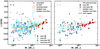Fig. 9.

Metallicity gradients vs. the stellar mass of the ATLAS^3D galaxies. Left-hand panel: all ATLAS^3D galaxies. Galaxies with cores are shown with red symbols, and core-less galaxies are represented in blue. The shape of the symbols indicates whether the galaxy is a slow (square) or a fast (circle) rotator. Diamonds show galaxies without HST imaging (empty) or with uncertain profiles (filled). NGC 1222 is shown as a green square. Red (dashed) and blue (solid) straight lines indicate the median values for core and core-less galaxies, respectively. The lengths of these lines are arbitrary and separated at mass of 10¹¹ M_⊙. The thick orange line is the running mean of Δ[Z/H]. Right-hand panel: focuses on the ATLAS^3D galaxies with HST imaging only, where coloured symbols are slow rotators, either with cores (red) or core-less (blue). Open symbols are fast rotators. Dashed lines indicate the median values for core and core-less galaxies, respectively. The thick red line is the best-fit relation for core slow rotators (red squares). Galaxies with cores tend to have shallow gradients, which flatten with the increase in mass, while core-less galaxies show a large spread.

The shallower gradients for more massive galaxies can be demonstrated by the running mean plotted in Fig. 9. The mean value of the gradient $\bar{Δ [Z / H]}$ $\overline{\Delta \mathrm{[Z/H]}}$ does not change for masses < 10¹¹ M_⊙, beyond which there is a gradual increase for about 0.1 dex, with a tendency for further increase. When we divide the sub-sample with HST imaging into galaxies that are less and more massive than 10¹¹ M_⊙, measure the median gradient and its standard deviation, we obtain the following values: the high-mass sub-sample has a median $\bar{Δ [Z / H]} = - 0.27 \pm 0.13$ $\overline{\Delta \mathrm{[Z/H]}} = -0.27 \pm 0.13$ , while the low-mass sub-sample has $\bar{Δ [Z / H]} = - 0.36 \pm 0.19$ $\overline{\Delta \mathrm{[Z/H]}} = -0.36 \pm 0.19$ . This is in line with predictions from numerical simulations that more massive galaxies should have flatter profiles. A very similar results is achieved when we calculate the median and the standard deviation of the gradients for core ( $\bar{Δ [Z / H]} = - 0.23 \pm 0.13$ $\overline{\Delta \mathrm{[Z/H]}} = -0.23 \pm 0.13$ ) and core-less galaxies ( $\bar{Δ [Z / H]} = - 0.36 \pm 0.15$ $\overline{\Delta \mathrm{[Z/H]}} = -0.36 \pm 0.15$ ), strengthening an assembly connection between the mass and the nuclear light structures.

Dividing galaxies according to their nuclear profiles and angular momentum adds important information (Table 4). As expected, both core slow rotators and core fast rotators are characterised by flatter metallicity gradients (close to −0.2), while core-less slow rotators and core-less fast rotators have steeper gradients (> − 0.35). Furthermore, the standard deviations of the metallicity gradients of core fast rotators, core-less fast rotators, and core-less slow rotators are similar among each other, ∼0.13 − 0.19, and to the values reported above. Significantly, the standard deviation of Δ[Z/H] for core slow rotators is only 0.07, at least a factor of 2 smaller. This tightening of the spread in metallicity gradients among core slow rotators is not visible when a selection in mass alone is considered, and we discuss this further.

Table 4.

Median values and scatter of the metallicity gradients for the galaxies in the ATLAS^3D sample.

The right-hand panel of Fig. 9 focuses on slow rotators. Here we again divided the core slow rotators and core-less slow rotators and plot in the background all other galaxies with HST imaging (fast rotators). This plot visualises the strong difference between core slow rotators and core-less slow rotators in terms of the dispersion of their Δ[Z/H] values. Core-less slow rotators can essentially have any value of Δ[Z/H] typical for the underlying fast rotators. Core slow rotators are located in a much more limited space of Δ[Z/H]. To quantify these differences in metallicity gradients, we performed a Kolmogorov-Smirnov test. The hypothesis that core slow rotators and core-less slow rotators are drawn from the same continuous distribution can be rejected because its probability is 0.0003. Similarly, the probability that metallicity gradients for core and core-less ATLAS^3D galaxies are drawn from the same distribution is only 0.001. A Kolmogorov-Smirnov test, however, cannot reject the hypothesis that core-less slow rotators and fast rotators in general are drawn from the same distribution (the rejection probability is 0.11).

Next to the conclusion that core slow rotators and core-less slow rotators (and galaxies in general) have different metallicity gradients, we see in the right-hand panel of Fig. 9 another interesting feature: there seems to be a correlation of the metallicity gradient of core slow rotators with their mass. We fitted a linear regression and found a relation Δ[Z/H] = 0.16log(M_⋆)−2.18, with correlation coefficient of 0.51. The correlation is not limited to the 15 core slow rotators in the ATLAS^3D sample because adding core fast rotators (9 galaxies) does not change its shape by much (Δ[Z/H] = 0.14log(M_⋆)−1.87). The correlation coefficient drops to 0.28, however, as expected because the dispersion of Δ[Z/H] of core fast rotators is significantly larger.

Figure 9 and Table 4 provide evidence for different formation scenarios between core slow rotators and other ETGs. The trend of flattening metallicity gradients with increasing mass is the dominant effect, seen both globally (in our full sample) and locally (among core slow rotators). Higher mass galaxies also have a lower dispersion of metallicity gradients, but when the selection is made for only core slow rotators, the spread in Δ[Z/H] is significantly minimised. The consequence of this small dispersion is that these galaxies must follow very similar formation scenarios, whereas the flat gradients suggest a lack of star formation in the assembly events. As a contrast, the steepness of the metallicity gradients of core-less galaxies are indicative of an inside-out formation, while the larger spread of the gradient values is indicative of more varied star-formation histories. Core fast rotators are somewhere in between the two extremes, having similar mean metallicity gradients like core slow rotators, but the dispersion of the gradients is more similar to core-less galaxies. The latter suggests that there are multiple ways of forming this class of galaxies.

We add two caveats pertinent to our sample. Firstly, there are only nine core slow rotators in the ATLAS^3D sample, and the results are susceptible to low number statistics. Secondly, above a mass of 2 − 3 × 10¹¹ M_⊙ there are no more fast rotators, and only core slow rotators remain. Selecting this mass cut would reproduce the same result as by selecting on core slow rotators, but for a small number of galaxies. Although we cannot fully separate the effects of galaxy mass, it plays a pivotal role. In Sect. 5 we discuss the influence of the mass on formation of flat metallicity gradients and cores in more detail.

4.4. Stellar age, age gradients, and star formation histories

We conclude our presentation of results by addressing the relation between the kinematics, surface brightness profiles, and age properties of stellar populations. For this purpose, we use the results of McDermid et al. (2015), specifically their SSP-based ages and α-element abundances within one effective radius (their Table 3). In Fig. 10 we focus on [α/Fe] abundances as a measure of the star formation timescales. Similar to Kormendy et al. (2009), we plot it against the effective velocity dispersion (as in Fig. 11 of McDermid et al. 2015), and after removing the best-fit relation, against the SSP ages. As before, we highlight the core and core-less galaxies as well as fast and slow rotators.

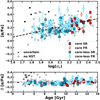Fig. 10.

Top: luminosity-weighted SSP α-element abundance vs. effective velocity dispersion of the ATLAS^3D galaxies. The dashed black line is the best-fit relation from McDermid et al. (2015, see their Table 5, relation i). Bottom: α-element abundance corrected for the σ_e dependance (by subtracting the values as given by the dashed line in the top panel) vs. the SSP age. Both SSP ages and [α/Fe] values are taken from McDermid et al. (2015), which also show that very old SSP ages are consistent with the fiducial age of the Universe (Planck Collaboration XIII 2016) when measurement errors and SSP mode uncertainties are taken into account. In both panels the symbols are the same and as described in the legend. Core-less slow rotators have a range of SSP ages, while core slow rotators as well as all but one core fast rotators are older than 10 Gyr.

The σ_e, or the mass, dependance of this relation is well known (e.g. Thomas et al. 2005), while Kormendy et al. (2009) also noted that core-less galaxies have lower α-elements abundances than core galaxies. This implies that the stars in core galaxies formed over a shorter timescale than stars in core-less galaxies. The ATLAS^3D sample shows a relatively large scatter in [α/Fe] – σ_e relation, where some of the largest [α/Fe], and therefore shortest star formation histories, are found among core-less fast rotators. When we focus only on slow rotators, however, they alone are consistent with the global relation (we take the best fit from McDermid et al. 2015, as given in their Table 5, where the slope and intercept are 0.31 ± 0.03 and −0.44 ± 0.05, respectively). Core-less slow rotators typically have lower [α/Fe]. This seems to be a purely σ_e driven effect because when the σ_e dependance is removed from the relation (bottom panel), there are no significant differences in relative abundances. In Sect. 5.3 we return to this point, but as gas-free merging cannot increase the value of [α/Fe], core-less slow rotators cannot be progenitors of core slow rotators, unlike some core-less fast rotators.

The bottom panel of Fig. 10 shows the distribution of light-weighted SSP ages. As already presented in McDermid et al. (2015), galaxies with complex kinematics (i.e. slow rotators) can have a range of ages. When core slow rotators and core-less slow rotators are separated, it becomes clear that slow rotators with the youngest stellar ages are found among core-less galaxies. Stars in core slow rotators are on average older than 10 Gyr, while core-less slow rotators can be as old as any ATLAS^3D galaxy. Notably, cores are found in galaxies with old stellar populations (with the exception of NGC 4382), regardless of whether they are fast or slow rotators. As the core formation occurred at or after the starburst (see Sect. 5.1), the formation redshift of cores is lower than 2−3.

In Fig. 11 we present the anti-correlation between the age and metallicity gradients. This is an expanded version of the plot presented in Kuntschner (2015). This time we add the information on the kinematics and the shape of the surface brightness profiles. Next to the strong anti-correlation between the age and metallicity gradients, consistent with other studies (e.g. Rawle et al. 2010; Koleva et al. 2011), this figure reveals a remarkable location of the core and core-less galaxies. Before we remark on them, we note that positive age gradients are expected to be produced by nuclear starbursts, which also enrich the medium and are responsible for the steepening of the negative metallicity gradients (Mihos & Hernquist 1994; Kobayashi 2004; Hopkins et al. 2009a). The overall anti-correlation in Fig. 11 is therefore expected and consistent with other stellar population relations (Kuntschner 2015; McDermid et al. 2015).

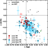Fig. 11.

Age gradients vs. metallicity gradient. Galaxies with cores are shown with red symbols, and core-less galaxies are represented in blue. The shape of the symbols indicates whether the galaxy is a slow (square) or a fast (circle) rotator. All galaxies follow an anti-correlation trend between the metallicity and age gradients. Core slow rotators are, however, found to have close to zero age gradients, while core-less slow rotators can have extreme positive and negative age gradients. Similar behaviour is observed for core fast rotator galaxies.

Figure 11 shows that core slow rotators have shallow age gradients (close to zero), while core-less slow rotators can essentially have any age gradient. They are found among galaxies with the most negative as well as most positive age gradients. This supports the conjecture where core-less slow rotators can be produced through a large variety of formation scenarios, while the formation of core slow rotators is much more restricted to a specific formation channel.

The location of core fast rotators is also noteworthy. These galaxies are distributed similarly to core-less slow rotators such as that there are some with negative age and nearly positive metallicity gradients, some with flat but negative metallicity and zero age gradients, and some with positive age and negative metallicity gradients. The implication is again that core fast rotators can be made through processes involving different levels of star formation and subsequent gas-poor merging that tend to flatten gradients.

5. Discussion

This section starts with reviews of the literature pertaining to the formation of stellar cores and flat metallicity gradient. Subsequently, we apply these ideas and the results presented above to outline possible scenarios for the formation of slow or fast and core or core-less galaxies. As a visual guide we show in Fig. 12 examples of surface brightness profiles and velocity maps of galaxy categories that we discuss here: a core slow rotator, a core fast rotator, a core-less slow rotator, and a core-less fast rotator.

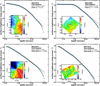Fig. 12.

Examples of four categories of galaxies with varied stellar kinematics and nuclear surface brightness profiles. In each panel, circular symbols show the nuclear surface brightness obtained in the same way as those in Figs. 1 and 2. The solid lines represent the Nuker fits with the gradient γ′ as given in the legend. Profiles and the Nuker fits for NGC 3379, NGC 3377, and NGC 4406 (data for this galaxy are from Ferrarese et al. 2006) are taken from Krajnović et al. (2013b), while data for NGC 3522 are from the present paper. The insets show respective velocity maps, demonstrating the level of regularity and some specific kinematic structures. The colour bars show the range of velocities, which are kept the same for all galaxies for comparison. Legends also provide details on the projected ellipticity and λ_Re, taken from Emsellem et al. (2011). The two fast rotators (left column) are characterised with regular rotation. The two slow rotators (right column) exhibit a KDC (top) and a CRC (bottom). The CRC in NGC 3522 has a peak rotation of only about 20 km s⁻¹ and is located within the central 5″ (Krajnović et al. 2011).

5.1. Formation of stellar cores

There are several possible scenarios for the creation of nuclear stellar cores, of which the most attention has been received by those involving the interaction of two supermassive black holes (SMBH; Begelman et al. 1980; Ebisuzaki et al. 1991; Makino & Ebisuzaki 1996; Quinlan 1996; Quinlan & Hernquist 1997; Milosavljević & Merritt 2001; Milosavljević et al. 2002; Merritt et al. 2007; Gualandris & Merritt 2012; Kulkarni & Loeb 2012; Rantala et al. 2018). The notion that the SMBH binaries are responsible for flat surface brightness profiles observed in bright ellipticals was first proposed by Faber et al. (1997). Following the work in numerical simulations (Barnes & Hernquist 1991, 1996; Mihos & Hernquist 1994), Faber et al. (1997) showed that core-less galaxies are consistent with being formed through dissipative, gas-rich mergers, but they also showed that pure dissipation-less, gas-poor mergers may not be able to form and maintain cores. Exploring an alternative model for core formation, Faber and collaborators proposed that SMBH binary mergers that remove stars from the nuclei could indeed explain the diversity of surface brightness profiles. Subsequent studies discovered that the SMBH mass correlates with the mass absent from the nuclei (Graham 2004; Ferrarese et al. 2006; Hyde et al. 2008; Kormendy & Bender 2009; Rusli et al. 2013; Dullo & Graham 2014), while Kormendy et al. (2009) summarised a myriad of evidence that core and core-less (extra light in their terminology) galaxies are products of dissipation-less and dissipative mergers, respectively, where SMBH binaries form cores.

The processes of core formation are based on the requirement that for an SMBH binary to become more tightly bound, it has to loose its angular momentum. The angular momentum is transferred to ejected stars that crossed the in-spiraling binary, which forms a depleted nuclear region. This results in the formation of a core in the light profile (Yu & Tremaine 2002; Milosavljević & Merritt 2003; Makino & Funato 2004; Merritt & Milosavljević 2005; Merritt 2006). Mergers without SMBHs show that the nucleus of the remnant is simply the denser of the progenitor nuclei (Holley-Bockelmann & Richstone 1999; Rantala et al. 2018). For the core formation in galactic mergers, two prerequisites are therefore necessary: two SMBHs, and an environment lacking cold gas. SMBHs will eject the stars depleting the core, but the paucity of gas will ensure the absence of a nuclear starburst that should refill the depleted region (e.g. Mihos & Hernquist 1994; Barnes & Hernquist 1996; Rothberg & Joseph 2004, 2006).

The reduction of the number of stars occurs before the SMBH merge, but it can continue even after the merger event. The anisotropic gravitational radiation can impart a recoil on the remnant SMBH of several hundred km s⁻¹, which then leaves the nucleus pulling along stars that are gravitationally bound to it. If the recoil velocity is not higher than the escape velocity, the SMBH will return to the nucleus as a result of dynamical friction, which will create an even larger core (Boylan-Kolchin et al. 2004; Merritt et al. 2004; Gualandris & Merritt 2008).

Overall, the formation of the core is a rapid process (within 50 Myr of the SMBH interaction, Rantala et al. 2018), and simulations indicate two straightforward observational predictions. One is the formation of the core, and the other is a tangentially anisotropic orbital distribution, as the core is depleted of orbits that cross the binary SMBH path (Quinlan et al. 1995; Quinlan & Hernquist 1997; Milosavljević & Merritt 2001; Rantala et al. 2018). The velocity anisotropy is indeed observable (e.g. Thomas et al. 2014, 2016), but only within the region dominated by the SMBH gravitational influence. A more readily observable kinematic consequence is a possibility of KDC formation from the interaction between the SMBHs and the surrounding stellar body. As SMBHs pass and exert torques on each other, there is a switch of the angular momentum between the SMBHs (and stars under their direct gravitational influence) and the rest of the galaxy, possibly producing nested KDCs (Rantala et al. 2019). Because the core formation is enhanced if the SMBHs are massive, and because such SMBHs live in massive galaxies (e.g. van den Bosch 2016), as well as because gas-poor mergers are more likely for massive, quiescent elliptical galaxies, we can expect that cores will be present in the most massive ETGs.

Finally, it should be noted that some of the processes invoked for the formation of cores in dark matter profiles (e.g. Goerdt et al. 2010; Laporte et al. 2012; Martizzi et al. 2012, 2013; Teyssier et al. 2013; Nipoti & Binney 2015; El-Zant et al. 2016), which depend on some sort of feedback mechanism, could also be at work in galactic nuclei. There is little evidence that their mechanisms and predicted properties are compatible with observed galactic nuclei, however.

5.2. Formation of flat metallicity gradients

Monolithic collapse models predict steep metallicity gradients (e.g. Pipino et al. 2008, 2010), while hierarchical merger models anticipate shallower gradients (e.g. Kobayashi 2004; Rupke et al. 2010). The metallicity gradients are strongly influenced by the amount of dissipation during the mass assembly, and, therefore an occurrence of a secondary star formation will steepen the gradients (e.g. Navarro-González et al. 2013). The mass ratio of the merger is important because equal-mass gas-free mergers are predicted to produce flatter metallicity gradients, while unequal mass mergers (e.g. with mass ratio of 1:5 or more) are shown to produce significant gradients at large radii (e.g. Hilz et al. 2012, 2013; Hirschmann et al. 2015). In such gas-free mergers, the flattening of the gradients also depends on the initial difference of the population gradients between the progenitors (Di Matteo et al. 2009). The scatter is also expected to be large depending on the efficiency of star formation and can be interpreted in terms of mergers of progenitors with various gas richness (Hopkins et al. 2009a,b) or in terms of the monolithic collapse model with differing star formation efficiency at a given mass (Pipino et al. 2010). Furthermore, a feedback mechanism (e.g. winds or AGN) is often necessary to align the simulation results with observations (e.g. Dubois et al. 2013; Hirschmann et al. 2015; Cook et al. 2016).

Notwithstanding the details and the absolute level of predicted metallicity gradients by models, a general conclusion is that galaxies undergoing dissipation-less merging will have flatter gradients than galaxies that experience gas-rich mergers or secondary star formation of any origin. This is important because we can link these predictions with formation scenarios for galaxies with cores (gas-poor major mergers) or for those with core-less light profiles (gas-rich mergers followed by a nuclear starburst). The expectation therefore is that galaxies with cores should have flatter metallicity gradients.

5.3. Formation of slow rotators with and without cores

The main implication of our results is that slow rotators can be divided into two sub-categories with different formation paths, which are revealed by their nuclear light profiles. The difference seems to be strongly related to the type of the merger at the most significant formation event. In the present and the following subsection, we build on the conclusions reached by Kormendy et al. (2009). We further probe a sample of galaxies focusing on the differences in their surface brightness profiles, adding critical information extracted from modern IFU data. The two-dimensional kinematics and stellar population properties provide us with an upgraded perspective, leading to new insights on core and core-less galaxies.

Core-less slow rotators have somewhat higher λ_r, lower σ_e, are typically flatter, less massive, and younger, with steeper metallicity gradients and a larger dispersion of the gradient values. Age gradients span the full range of slopes from steep positive over flat to steep negative values. The detailed kinematic properties show that they have a more significant anti-correlation between V/σ and h₃, and exclusively have 2σ type of kinematics. These last two aspects suggest that at least for some of them (40−45% according to the discussion in Sect. 4.1), the low angular momentum is a consequence of the counter-rotation of flattened structures. These are not necessarily actual discs, but are characterised as having well-defined angular momentum vectors, oriented in opposite directions. Crucially, they have lower masses than the core slow rotators. They are therefore more closely linked in their evolution to fast rotators (Sect. 3.4.3 of Cappellari 2016).

Following theoretical predictions and previous observational work (e.g. Kormendy et al. 2009), we conclude that core-less slow rotators are mostly products of gas-rich interactions. Some might form by accretion of counter-rotating and star-forming gas (e.g. Algorry et al. 2014; Coccato et al. 2015; Starkenburg et al. 2019), where the number of counter-rotating stars that formed defines whether the galaxy is classified as a slow rotator. Other core-less slow rotators might form in gas-rich mergers of specific orbital configuration. NGC 1222 is likely an example of such a merger. This gas-rich merger is in an advanced stage (Young et al. 2018), but the outcome is not yet fully defined. It can, however, be expected that the remnant will have a low net angular momentum, with possibly a KDC or even a prolate-like rotation, but likely with a core-less light profile (e.g. Rothberg & Joseph 2004, 2006). Finally, equal-mass binary mergers (e.g. Bournaud et al. 2005; Bois et al. 2011) showed that stellar discs might survive if the orbital orientations and the intrinsic spins of progenitors are finely tuned. This is most likely the formation scenario of the prototypical 2σ galaxy and a core-less slow rotator NGC 4550 (Crocker et al. 2009).

McDermid et al. (2015) showed that galaxies with non-regular kinematics (typically slow rotators) fall below the general trend in a [Z/H] versus σ_e (see their Fig. 11). The trend is more pronounced for galaxies with lower σ_e and lower mass, which effectively selects our core-less slow rotators. As the authors argued, this can be considered as an offset in metallicity (these galaxies are less metal rich than typical fast rotators), or an offset in velocity dispersion or mass (have larger velocity dispersion or higher mass for a given metallicity). The latter can be understood as a consequence of a merger in which violent relaxation (Lynden-Bell 1967; Spergel & Hernquist 1992) plays a major role in reshaping the internal structure of galaxies (Hilz et al. 2012) as well as morphologically transform galaxies (Hernquist 1993). This applies to minor collisional and major collision-less mergers (Naab & Ostriker 2017).

Mergers producing core-less slow rotators are between progenitors, with the mass ratios spanning a significant range (e.g. 1:1−1:10), but the orbital configurations of the mergers must be such to produce low angular momentum remnants (e.g. Naab et al. 2006a, 2014; Hoffman et al. 2009, 2010; Bois et al. 2011; Moody et al. 2014; Röttgers et al. 2014; Lagos et al. 2018). In some of these mergers, a binary SMBH pair might form, but it could be of too low mass⁷ to excavate an observable core (Rantala et al. 2018), or the central starburst is able to refill the nuclei (Mihos & Hernquist 1994; Kormendy et al. 2009, see also Sect. 5.4). Finally, radiative feedback from the active galactic nucleus, or a mechanical feedback from winds, can also facilitate the production of slow rotators by preventing the cooling and accretion of new gas (Serra et al. 2014; Frigo et al. 2019).

Steeper metallicity gradients of core-less slow rotators are compatible with these formation scenarios. Crucially, the fact that the gradients show a large dispersion indicates that there are multiple pathways for the formation of core-less slow rotators. Even a range of star formation histories is allowed, as long as new stars do not settle in a fast, co-rotating, and flat disc-like structure. The formation channels are characterised by the fact that the progenitors are typically less massive (∼10¹⁰ M_⊙ or smaller), have different stellar populations (typical of fast rotators), and have various amounts of gas.

Core slow rotators are more massive galaxies, with the lowest angular momenta, show flat age and metallicity gradients, and are made of old stellar populations. They comprise systems of the highest σ_e, and some of them show no net rotation. Such properties are predicted from major and multiple minor dissipation-less mergers (e.g. Jesseit et al. 2005; Naab et al. 2006b, 2009; Moody et al. 2014; Röttgers et al. 2014; Lagos et al. 2018; Rantala et al. 2018). Furthermore, these properties also require a very active mass-assembly history, rich in accretion of much smaller galaxies (e.g. Hilz et al. 2013), but also experiencing a few major (equal mass) mergers (e.g. De Lucia & Blaizot 2007). The latter are required in order to produce complex kinematics and also to create cores in the nuclei through binary supermassive black hole evolution (Faber et al. 1997; Kormendy et al. 2009; Rantala et al. 2018). The location of core slow rotators in the mass - size diagram is consistent with the predicted location of remnants of equal-mass dissipation-less mergers (Boylan-Kolchin et al. 2006; Bezanson et al. 2009; Naab et al. 2009; Hopkins et al. 2009c), which indicates a doubling growth in mass and size, but no change in the effective velocity dispersion. This remains true for galaxies with masses higher than 10¹² M_⊙ (Krajnović et al. 2018a; Graham et al. 2018).

Numerical simulations placed in the cosmological context (see the review by Naab & Ostriker 2017) produce consistent results with simulations of binary mergers. Massive galaxies are gas-poor systems, and their late evolution (z < 2) is dominated by accretion of stars formed elsewhere (e.g. De Lucia & Blaizot 2007; Oser et al. 2010; Wellons et al. 2015; Cook et al. 2016; Lagos et al. 2018). The current picture is that low-mass galaxies typically grow through star formation and are more likely to experience dissipative mergers, while massive galaxies accrete stars formed elsewhere and grow through dissipation-less mergers (e.g. Rodriguez-Gomez et al. 2016; Qu et al. 2017). Empirical models support this picture (Moster et al. 2013, 2018; Behroozi et al. 2013). The implication is that the SMBH masses will also increase proportionally to the SMBH masses of progenitors and the number of subsequent gas-free mergers. This gives rise to the relation of the SMBH mass with the core size, as well as with the missing light (or stellar mass) compared to the extrapolation of an external light profile (Graham 2004; Lauer et al. 2007; Kormendy et al. 2009; Rusli et al. 2013). It also supports the expectation that the SMBH mass will not correlate well only with the velocity dispersion in the most massive systems (Krajnović et al. 2018b).

Core slow rotators are consistent with being merger remnants of galaxies that resemble present-epoch massive core-less fast rotators or core slow rotators. This is supported by the overlap in [α/Fe] values (Fig. 10) for some core-less fast rotators and core slow rotators and by the substantial population of core-less fast rotators with large σ_e (and masses, Fig. 7). Furthermore, there are also core fast rotators that overlap in σ_e and [α/Fe] (as well as mass) with core slow rotators. This is important because during the dissipation-less major merging, the velocity dispersion typically remains unchanged. On the other hand, core-less slow rotators do not seem to be able to contribute to the formation of core slow rotators and the most massive galaxies in general. Their σ_e and [α/Fe] are too low. This conclusion is similar to that reached by Kormendy et al. (2009), but our spectroscopic data provide stronger constraints on types of possible progenitors of core slow rotators.

Galaxy mergers, the lack of cold gas, and the interaction of massive SMBHs seems to be crucial for the creation of cores. This is typical for the most massive galaxies, as is the low angular momentum that is expected to result from such interactions. Moreover, the flat metallicity gradients and the small variation between them imply a unique channel of formation or a few different formation paths that have a dominant physical process in common: dynamical mixing of stellar populations is efficient and likely dependent on mass. Furthermore, maintaining the core is necessary, and this is probably why cores are mostly found in massive slow rotators: they are able to retain their halo of hot X-ray emitting gas (Kormendy et al. 2009; Krajnović et al. 2013b).

5.4. Formation of fast rotators with cores

Core fast rotators, while comprising only a small fraction of fast rotators (9 of 111 ATLAS^3D fast rotators with HST imaging), seem to contradict the favoured scenario of core formation. Krajnović et al. (2013b) showed that core fast rotators often have regular kinematics and a significant V/σ − h₃ anti-correlation. These are indicative of embedded disc-like structures. Core fast rotators have somewhat lower masses and σ_e, but a significant overlap also exists with the properties of core slow rotators (e.g. see Fig. 7). Judging by many other galaxy properties, such as stellar populations, age, metallicity gradients, α-element abundances (as presented in this paper), molecular gas content, mass of supermassive black holes, or derived core parameters (as presented in Krajnović et al. 2013b), core fast rotators are similar to core slow rotators. Two more notable differences with respect to core slow rotators deserve to be highlighted. Firstly, core fast rotators show a large dispersion in metallicity and age gradients, indicating that they can be formed in different ways (Sects. 4.3 and 4.4). Secondly, core fast rotators have a lower X-ray emission than core slow rotators, but it is similar to those of core-less galaxies (Krajnović et al. 2013b). This means that at least a theoretically, they might accrete cold gas after the last merger s(and the formation of the core) and change their global kinematics.

At this point it is instructive to consider some of these galaxies in more detail. NGC 0524 and NGC 4473 have very clear evidence for embedded discs, both morphologically and kinematically. NGC 0524, has a nuclear dust disc which makes the analysis of the nuclear light profile difficult, but is the only core galaxy with molecular gas (Young et al. 2011), while dynamical models for NGC 4473 require two counter-rotating discs (Cappellari et al. 2007). The cores in these two galaxies seem to be well defined, but the cores might also depend on the actual choice of the fitting range. For example, Kormendy et al. (2009) showed that in the case of NGC 4473, it is possible to fit the surface brightness profile such as to recover a core, an extra-light (core-less) or a combination of an extra-light profile with an indication for a core (their Figs. 58 (top), 17, and 58 (bottom), respectively). This suggests that some of core fast rotators could be considered as just somewhat unusual fast rotators.

Alternative examples are provided by NGC 4649 and NGC 5485. The former is the third most luminous galaxy in the Virgo cluster and the latter has a prolate-like (around the major axis) rotation (Krajnović et al. 2011). These two galaxies are massive and have relatively high σ_e. This is especially the case for NGC 4649, which is one of the most massive galaxies in the ATLAS^3D sample, the most massive fast rotator (see Fig 7), and also has one of highest σ_e in the sample. The prolate-like rotation of NGC 5485 requires a special merging configuration, possibly favouring a dissipation-less type of merger as it also has a nuclear gas disc in polar configuration (Tsatsi et al. 2017; Ebrová & Łokas 2017; Li et al. 2018b). These galaxies are much more similar to core slow rotators, and it is possible that their classification depends on the definition of fast rotators as much as their angular momenta depend on the chance outcome of the formation process.

Possible scenarios for the formation of core fast rotators are limited by two constraints: they show cores, and they show increased angular momentum and often evidence for discs. On the other hand, as has been argued by Faber et al. (1997) and Kormendy et al. (2009), given that almost all bright galaxies contain SMBHs, the question is not why some galaxies have cores, but why most of galaxies are core-less. Their explanation, supported by simulations and other observations (as cited above), is that in a major merger a central starburst will fill any core excavated by the interacting black holes. This might not be the complete picture because we do not yet have full understanding of the specific conditions relevant to ejection of stars by the binary SMBHs, or starburst physics. In particular, the duration of a nuclear starburst can be as short as 30−50 Myr (e.g. Renaud et al. 2014; Fensch et al. 2017), while the core excavation is completed on a comparable timescale (∼50 Myr, Rantala et al. 2018), and both processes are likely to be strongly dependant on the initial conditions (i.e. gas mass, SMBH mass, merger orbital set-up, and feedback Naab & Ostriker 2017).

Furthermore, it is useful to recall that some core slow rotators could also be created through dissipative mergers. NGC 5557 is one such case (Duc et al. 2011), a relatively massive (2 × 10¹¹ M_⊙) and round core slow rotator. This galaxy, very typical of slow rotators in its central regions, has a long and narrow tidal tail featuring gas-rich and star-forming objects, which are likely tidal dwarf galaxies. The long-lived tidal structures in NGC 5557 are likely related to the event that formed the present galaxy, as the luminosity-weighted stellar age in the central regions is only 1−2 Gyr old, even though no evidence of a starburst remains and the surface brightness core is detectable. NGC 5557 is likely a special case and could have ended as a core fast rotator. Nevertheless, this case, as well as many of the core fast rotators, should add caution to our discussion because our understanding of the assembly process through dissipative and dissipation-less processes is evidently incomplete.

We reiterate previous suggestions that core fast rotators are the galaxies that experienced a shorter central starburst compared to the time of the binary SMBH evolution. They are characterised with (typically) lower masses, diverse stellar population parameters, and lower X-ray luminosities. This makes them candidate remnants of dissipative mergers, where the final outcome (i.e. core or core-less, fast or slow rotator) could depend on initial conditions such as the gas mass, black hole mass, feedback, or general details of the merger. Furthermore, as shown by Bois et al. (2011), dissipation-less mergers can also result in fast rotators (see also Moody et al. 2014; Naab et al. 2014) and core fast rotators might just be special cases, curious products of the vast parameter space of merger orbits.

6. Conclusions

We used SAURON IFU observations and HST imaging of the ATLAS^3D sample to investigate the formation of early-type galaxies. In particular, we presented the metallicity and age gradients for the full ATLAS^3D sample. We also link this paper with a public release of the age, metallicity, and α-element abundance profiles, SAURON maps of the SSP equivalent stellar age, metallicity, and α-element abundances, which can be obtained from the ATLAS^3D website. Furthermore, this paper presents the analysis of the HST imaging of 12 ATLAS^3D Survey slow rotators. We derived their nuclear stellar surface brightness profiles except for one galaxy that was too dusty. Combining these with results of Krajnović et al. (2013b) and the kinematic properties of ATLAS^3D galaxies, we divided the ATLAS^3D galaxies into core slow rotators, core-less slow rotators, core fast rotators, and core-less fast rotators. The last category is the most numerous, but it is also the most incomplete with respect to the HST imaging. Nevertheless, this study presents the first complete volume-limited sample of slow rotators with IFU kinematics and high spatial resolution photometry.

Using the Nuker profile parametrisation, we showed that all newly analysed slow rotators have rising light profiles and can be classified as core-less. We placed an upper limit on the core sizes of ∼10 pc. Because there are no known galaxies with smaller cores, our observations are consistent with expectations and show that lower mass slow rotators do not harbour unexpected nuclear structures. This allowed us to show that more than half (about 55%) of the slow rotators in the ATLAS^3D sample have core-less light profiles.

The metallicity gradients of the ATLAS^3D galaxies are consistent with gradients expected for galaxies in the same mass range. We detect a trend where the most massive galaxies (> 10¹¹ M_⊙) show significantly flatter gradients ( $\bar{Δ [Z / H]} = - 0.28$ $\overline{\Delta \mathrm{[Z/H]}} =-0.28$ ) than the less massive galaxies ( $\bar{Δ [Z / H]} = - 0.37$ $\overline{\Delta \mathrm{[Z/H]}} =-0.37$ ). This is closely reflected for galaxies with core and core-less light profiles ( $\bar{Δ [Z / H]} = - 0.23$ $\overline{\Delta \mathrm{[Z/H]}} =-0.23$ and −0.36, respectively). Core slow rotators and core fast rotators have similarly flat gradients (−0.23 and −0.19, respectively), but the dispersion of gradient values is much higher for core fast rotators (0.19 compared to 0.07). The mean gradient and gradient dispersion values of core-less slow rotators are similar to those of core-less fast rotators. There is also an indication that metallicity gradients become flatter with increasing mass. Age gradients of core slow rotators are close to zero, while those of core-less slow rotators or core fast rotators can take essentially any value as the underlying ETG population.

The presence (or absence) of cores correlates with a number of other properties of slow rotators. We find that core-less slow rotators, compared to core slow rotators

are less massive (typically < 10¹¹ M_⊙), have lower σ_e and overlap with fast rotators in the mass – size diagram,
are flatter, have somewhat higher λ_R, and often show evidence of counter-rotation, and
have steeper metallicity gradients $(\bar{Δ [Z / H]} = - 0.42$ $(\overline{\Delta \mathrm{[Z/H]}} =-0.42$ compared to $\bar{Δ [Z / H]} = - 0.23)$ $\overline{\Delta \mathrm{[Z/H]}} =-0.23)$ , and show a large dispersion of gradient values (δ(Δ[Z/H]) = 0.18 compared to δ(Δ[Z/H]) = 0.07) as well as a range of stellar ages.

Core slow rotators are extreme galaxies. They are the brightest and most massive, the largest, and have the highest σ_e. They have the lowest angular momenta. Their stellar populations (within one half-light radius) are always old, and the metallicity gradients are shallow and show little dispersion. There is an indication that the metallicity gradients flatten with increasing mass.

Core-less slow rotators and core slow rotators are equally likely to have KDCs or CRCs, but velocity maps with no net rotation are obtained only for core slow rotators, while 2σ velocity dispersion maps are exclusive for core-less slow rotators. From investigating also the higher order moments of the LOSVD, we conclude that core-less slow rotators form due to accretion of counter-rotating star-forming gas or stars, and the level of the counter-rotation defines whether they are classified as slow rotators. A fraction of core-less slow rotators are remnants of dissipational processes, such as gas-rich mergers of various mass ratios with specific orbital configurations, which can also decrease the net angular momentum of the remnant. Violent relaxation can also influence the formation of core-less slow rotators.

Core fast rotators share some properties with core slow rotators (i.e. presence of cores, [α/Fe], mass, σ_e, mean values of metallicity gradients, and old ages) and some properties with core-less slow rotator and other fast rotators (i.e. kinematics, counter-rotation, disc-like components, higher λ_R, larger spread in metallicity and age gradients, and lower X-ray luminosities). In this respect, core fast rotators are the most diverse class in terms of possible formation channels. They can be products of gas-poor mergers that result in fast rotators (but allow core creation), gas-rich mergers with a central starburst of shorter duration than the binary SMBH evolution, or are able to subsequently increase angular momentum through further interactions without destroying cores. Most likely, every such galaxy will have a unique way of mass assembly, core formation, and subsequent protection.

In contrast to all this, the formation of core slow rotators requires at least one and probably a few dissipation-less major mergers in the presence of massive black holes in order to produce the core, flatten their metallicity gradients, and create the variety of observed kinematics. Their progenitors could be galaxies resembling present-day core fast rotators or most massive core-less fast rotators, but the assembly of the most massive galaxies is only possible by core slow rotators themselves.

Our results support the approach of only considering core slow rotators when searching for massive dry merger relics in observations (Lauer 2012; Cappellari 2013) or when describing their evolution as a class (Cappellari 2016). Finally, the fact that core slow rotators only dominate the characteristic mass of M_crit ∼ 2 × 10¹¹ M_⊙ and are completely absent below ∼10¹¹ M_⊙ indicates that when the characteristics (e.g. their shapes or environments) of massive dry merger relics are to be studied but high-resolution imaging is not available, a further removal of spurious objects is easily achieved by removing slow rotators below M_crit (e.g. Li et al. 2018c).

¹

λ_Re measures the project and specific (weighted by a mass proxy) angular momentum within one half-radius. Several studies noted that assuming a different scale, the relative values of λ_Re can change (Arnold et al. 2014; Foster et al. 2016; Bellstedt et al. 2017; Graham et al. 2017). A scale is a natural requirement for any classification. The one effective radius was driven by the size of the IFU, the distance of the galaxies, and their brightness. As we work on galaxies from Emsellem et al. (2011), we retain their definition.

²

The term “cusps” is sometimes used as a description of steep central surface brightness profiles (e.g. Sparke & Gallagher 2000, p. 238). However, some confusion may emerge when the “cuspy cores” is used as in Kormendy et al. (2009). In order to avoid any ambiguity, we prefer to use core-less as a direct opposite to core.

³

http://purl.org/atlas3d

⁴

Resolvable via https://doi.org/10.17876/data/2020_1

⁵

https://www.spacetelescope.org/images/potw1645a/

⁶

Velocity maps characterised as NRR by Krajnović et al. (2011) have a relatively low rotation amplitude, an irregular appearance, and possible kinematic twists. These all result in deviations from the regular rotation (as found in fast rotators) that is described by a simple disc-like velocity model.

⁷

Core-less slow rotators have masses between 10¹⁰ and 10¹¹ M_⊙, which implies black hole masses of ∼10⁷ up to 10⁸ M_⊙ (e.g. van den Bosch 2016).

Acknowledgments

Michael Wolfe deceased during the final stages of this work, due to complications resulting from a stroke. He was very friendly to everyone, dedicated to his work, and always eager to learn new things. We offer sincere condolences to his family and friends. DK acknowledges support from the grant GZ: KR 4548/2-1 of the Deutsche Forschungsgemeinschaft. UU acknowledges support from the grant 50 OR 1412 of the Deutsches Zentrum für Luft- und Raumfahrt. MC acknowledges support from a Royal Society University Research Fellowship. RMcD is the recipient of an Australian Research Council Future Fellowship (project number FT150100333). RLD acknowledges travel and computer grants from Christ Church, Oxford, and support from the Oxford Hintze Centre for Astrophysical Surveys, which is funded through generous support from the Hintze Family Charitable Foundation. Support for this project was provided by NASA through grant HST-GO-13324 from the Space Telescope Science Institute, which is operated by the Association of Universities for Research in Astronomy, Inc., under NASA contract NAS5-26555.

References

Algorry, D. G., Navarro, J. F., Abadi, M. G., et al. 2014, MNRAS, 437, 3596 [NASA ADS] [CrossRef] [Google Scholar]
Arnold, J. A., Romanowsky, A. J., Brodie, J. P., et al. 2014, ApJ, 791, 80 [NASA ADS] [CrossRef] [Google Scholar]
Bacon, R., Copin, Y., Monnet, G., et al. 2001, MNRAS, 326, 23 [NASA ADS] [CrossRef] [Google Scholar]
Barnes, J. E., & Hernquist, L. E. 1991, ApJ, 370, L65 [NASA ADS] [CrossRef] [Google Scholar]
Barnes, J. E., & Hernquist, L. 1996, ApJ, 471, 115 [NASA ADS] [CrossRef] [Google Scholar]
Begelman, M. C., Blandford, R. D., & Rees, M. J. 1980, Nature, 287, 307 [NASA ADS] [CrossRef] [Google Scholar]
Behroozi, P. S., Wechsler, R. H., & Conroy, C. 2013, ApJ, 770, 57 [NASA ADS] [CrossRef] [Google Scholar]
Bellstedt, S., Forbes, D. A., Foster, C., et al. 2017, MNRAS, 467, 4540 [NASA ADS] [CrossRef] [Google Scholar]
Bender, R., & Nieto, J. 1990, A&A, 239, 97 [NASA ADS] [Google Scholar]
Bender, R., Saglia, R. P., & Gerhard, O. E. 1994, MNRAS, 269, 785 [NASA ADS] [CrossRef] [Google Scholar]
Bendo, G. J., & Barnes, J. E. 2000, MNRAS, 316, 315 [NASA ADS] [CrossRef] [Google Scholar]
Bertin, E., & Arnouts, S. 1996, A&AS, 117, 393 [NASA ADS] [CrossRef] [EDP Sciences] [Google Scholar]
Bertola, F., & Capaccioli, M. 1975, ApJ, 200, 439 [NASA ADS] [CrossRef] [Google Scholar]
Bezanson, R., van Dokkum, P. G., Tal, T., et al. 2009, ApJ, 697, 1290 [NASA ADS] [CrossRef] [Google Scholar]
Binney, J. 1978, MNRAS, 183, 501 [NASA ADS] [Google Scholar]
Binney, J. 2005, MNRAS, 363, 937 [NASA ADS] [CrossRef] [Google Scholar]
Binney, J., & Tremaine, S. 2008, Galactic Dynamics, 2nd edn. (Princeton, NJ: Princeton University Press) [Google Scholar]
Bois, M., Emsellem, E., Bournaud, F., et al. 2011, MNRAS, 416, 1654 (Paper VI) [NASA ADS] [CrossRef] [Google Scholar]
Bonfini, P., & Graham, A. W. 2016, ApJ, 829, 81 [NASA ADS] [CrossRef] [Google Scholar]
Bournaud, F., Jog, C. J., & Combes, F. 2005, A&A, 437, 69 [NASA ADS] [CrossRef] [EDP Sciences] [Google Scholar]
Boylan-Kolchin, M., Ma, C.-P., & Quataert, E. 2004, ApJ, 613, L37 [NASA ADS] [CrossRef] [Google Scholar]
Boylan-Kolchin, M., Ma, C.-P., & Quataert, E. 2006, MNRAS, 369, 1081 [NASA ADS] [CrossRef] [Google Scholar]
Bracewell, R. N., & Roberts, J. A. 1954, Aust. J. Phys., 7, 615 [NASA ADS] [CrossRef] [Google Scholar]
Brough, S., Tran, K.-V., Sharp, R. G., von der Linden, A., & Couch, W. J. 2011, MNRAS, 414, L80 [NASA ADS] [CrossRef] [Google Scholar]
Brough, S., van de Sande, J., Owers, M. S., et al. 2017, ApJ, 844, 59 [NASA ADS] [CrossRef] [Google Scholar]
Burger, H. C., & van Cittert, P. H. 1932, Z. Phys., 79, 722 [NASA ADS] [CrossRef] [Google Scholar]
Byun, Y.-I., Grillmair, C. J., Faber, S. M., et al. 1996, AJ, 111, 1889 [NASA ADS] [CrossRef] [Google Scholar]
Caon, N., Capaccioli, M., & D’Onofrio, M. 1993, MNRAS, 265, 1013 [NASA ADS] [CrossRef] [Google Scholar]
Cappellari, M. 2013, ApJ, 778, L2 [NASA ADS] [CrossRef] [Google Scholar]
Cappellari, M. 2016, ARA&A, 54, 597 [NASA ADS] [CrossRef] [Google Scholar]
Cappellari, M., Emsellem, E., Bacon, R., et al. 2007, MNRAS, 379, 418 [NASA ADS] [CrossRef] [Google Scholar]
Cappellari, M., Emsellem, E., Krajnović, D., et al. 2011a, MNRAS, 413, 813 (Paper I) [NASA ADS] [CrossRef] [Google Scholar]
Cappellari, M., Emsellem, E., Krajnović, D., et al. 2011b, MNRAS, 416, 1680 (Paper VII) [NASA ADS] [CrossRef] [Google Scholar]
Cappellari, M., Scott, N., Alatalo, K., et al. 2013a, MNRAS, 432, 1709 [NASA ADS] [CrossRef] [Google Scholar]
Cappellari, M., McDermid, R. M., Alatalo, K., et al. 2013b, MNRAS, 432, 1862 [NASA ADS] [CrossRef] [Google Scholar]
Carollo, C. M., Franx, M., Illingworth, G. D., & Forbes, D. A. 1997, ApJ, 481, 710 [NASA ADS] [CrossRef] [Google Scholar]
Coccato, L., Fabricius, M., Morelli, L., et al. 2015, A&A, 581, A65 [NASA ADS] [CrossRef] [EDP Sciences] [Google Scholar]
Cook, B. A., Conroy, C., Pillepich, A., Rodriguez-Gomez, V., & Hernquist, L. 2016, ApJ, 833, 158 [NASA ADS] [CrossRef] [Google Scholar]
Crane, P., Stiavelli, M., King, I. R., et al. 1993, AJ, 106, 1371 [NASA ADS] [CrossRef] [Google Scholar]
Crocker, A. F., Jeong, H., Komugi, S., et al. 2009, MNRAS, 393, 1255 [NASA ADS] [CrossRef] [Google Scholar]
Davies, R. L., & Illingworth, G. 1983, ApJ, 266, 516 [NASA ADS] [CrossRef] [Google Scholar]
Davies, R. L., Efstathiou, G., Fall, S. M., Illingworth, G., & Schechter, P. L. 1983, ApJ, 266, 41 [NASA ADS] [CrossRef] [Google Scholar]
De Lucia, G., & Blaizot, J. 2007, MNRAS, 375, 2 [NASA ADS] [CrossRef] [Google Scholar]
de Zeeuw, T., & Franx, M. 1991, ARA&A, 29, 239 [NASA ADS] [CrossRef] [Google Scholar]
de Zeeuw, P. T., Bureau, M., Emsellem, E., et al. 2002, MNRAS, 329, 513 [NASA ADS] [CrossRef] [Google Scholar]
Di Matteo, P., Pipino, A., Lehnert, M. D., Combes, F., & Semelin, B. 2009, A&A, 499, 427 [NASA ADS] [CrossRef] [EDP Sciences] [Google Scholar]
D’Onofrio, M., Capaccioli, M., & Caon, N. 1994, MNRAS, 271, 523 [NASA ADS] [CrossRef] [Google Scholar]
Dressler, A., & Sandage, A. 1983, ApJ, 265, 664 [NASA ADS] [CrossRef] [Google Scholar]
Dubois, Y., Pichon, C., Devriendt, J., et al. 2013, MNRAS, 428, 2885 [NASA ADS] [CrossRef] [Google Scholar]
Dubois, Y., Peirani, S., Pichon, C., et al. 2016, MNRAS, 463, 3948 [NASA ADS] [CrossRef] [Google Scholar]
Duc, P. A., Cuillandre, J. C., Serra, P., et al. 2011, MNRAS, 417, 863 (Paper IX) [NASA ADS] [CrossRef] [Google Scholar]
Dullo, B. T., & Graham, A. W. 2012, ApJ, 755, 163 [NASA ADS] [CrossRef] [Google Scholar]
Dullo, B. T., & Graham, A. W. 2013, ApJ, 768, 36 [NASA ADS] [CrossRef] [Google Scholar]
Dullo, B. T., & Graham, A. W. 2014, MNRAS, 444, 2700 [NASA ADS] [CrossRef] [Google Scholar]
Dullo, B. T., Graham, A. W., & Knapen, J. H. 2017, MNRAS, 471, 2321 [NASA ADS] [CrossRef] [Google Scholar]
Ebisuzaki, T., Makino, J., & Okumura, S. K. 1991, Nature, 354, 212 [NASA ADS] [CrossRef] [Google Scholar]
Ebrová, I., & Łokas, E. L. 2017, ApJ, 850, 144 [NASA ADS] [CrossRef] [Google Scholar]
Efstathiou, G., Ellis, R. S., & Carter, D. 1980, MNRAS, 193, 931 [NASA ADS] [CrossRef] [Google Scholar]
Efstathiou, G., Ellis, R. S., & Carter, D. 1982, MNRAS, 201, 975 [NASA ADS] [Google Scholar]
El-Zant, A. A., Freundlich, J., & Combes, F. 2016, MNRAS, 461, 1745 [NASA ADS] [CrossRef] [Google Scholar]
Emsellem, E., Cappellari, M., Krajnović, D., et al. 2007, MNRAS, 379, 401 [NASA ADS] [CrossRef] [Google Scholar]
Emsellem, E., Cappellari, M., Krajnović, D., et al. 2011, MNRAS, 414, 888 (Paper III) [NASA ADS] [CrossRef] [Google Scholar]
Faber, S. M., Tremaine, S., Ajhar, E. A., et al. 1997, AJ, 114, 1771 [NASA ADS] [CrossRef] [Google Scholar]
Fensch, J., Renaud, F., Bournaud, F., et al. 2017, MNRAS, 465, 1934 [NASA ADS] [CrossRef] [Google Scholar]
Ferrarese, L., van den Bosch, F. C., Ford, H. C., Jaffe, W., & O’Connell, R. W. 1994, AJ, 108, 1598 [NASA ADS] [CrossRef] [Google Scholar]
Ferrarese, L., Côté, P., Jordán, A., et al. 2006, ApJS, 164, 334 [NASA ADS] [CrossRef] [Google Scholar]
Ford, H. C., Bartko, F., Bely, P. Y., et al. 1998, in Society of Photo-Optical Instrumentation Engineers (SPIE) Conference Series, eds. P. Y. Bely, & J. B. Breckinridge, 3356, 234 [NASA ADS] [Google Scholar]
Foster, C., Pastorello, N., Roediger, J., et al. 2016, MNRAS, 457, 147 [NASA ADS] [CrossRef] [Google Scholar]
Franx, M., Illingworth, G., & Heckman, T. 1989, ApJ, 344, 613 [NASA ADS] [CrossRef] [Google Scholar]
Franx, M., Illingworth, G., & de Zeeuw, P. T. 1991, ApJ, 383, 112 [NASA ADS] [CrossRef] [Google Scholar]
Frigo, M., Naab, T., Hirschmann, M., et al. 2019, MNRAS, 489, 2702 [NASA ADS] [CrossRef] [Google Scholar]
Glass, L., Ferrarese, L., Côté, P., et al. 2011, ApJ, 726, 31 [NASA ADS] [CrossRef] [Google Scholar]
Goddard, D., Thomas, D., Maraston, C., et al. 2017, MNRAS, 466, 4731 [NASA ADS] [Google Scholar]
Goerdt, T., Moore, B., Read, J. I., & Stadel, J. 2010, ApJ, 725, 1707 [NASA ADS] [CrossRef] [Google Scholar]
González Delgado, R. M., García-Benito, R., Pérez, E., et al. 2015, A&A, 581, A103 [NASA ADS] [CrossRef] [EDP Sciences] [Google Scholar]
González-García, A. C., Balcells, M., & Olshevsky, V. S. 2006, MNRAS, 372, L78 [NASA ADS] [CrossRef] [Google Scholar]
Graham, A. W. 2001, AJ, 121, 820 [NASA ADS] [CrossRef] [Google Scholar]
Graham, A. W. 2004, ApJ, 613, L33 [NASA ADS] [CrossRef] [Google Scholar]
Graham, A., Lauer, T. R., Colless, M., & Postman, M. 1996, ApJ, 465, 534 [NASA ADS] [CrossRef] [Google Scholar]
Graham, A. W., Erwin, P., Trujillo, I., & Asensio Ramos, A. 2003, AJ, 125, 2951 [NASA ADS] [CrossRef] [Google Scholar]
Graham, A. W., Janz, J., Penny, S. J., et al. 2017, ApJ, 840, 68 [NASA ADS] [CrossRef] [Google Scholar]
Graham, M. T., Cappellari, M., Li, H., et al. 2018, MNRAS, 477, 4711 [NASA ADS] [CrossRef] [Google Scholar]
Graham, M. T., Cappellari, M., Bershady, M. A., & Drory, N. 2019, A&A, submitted [arXiv:1910.05139] [Google Scholar]
Greene, J. E., Leauthaud, A., Emsellem, E., et al. 2017, ApJ, 851, L33 [NASA ADS] [CrossRef] [Google Scholar]
Gualandris, A., & Merritt, D. 2008, ApJ, 678, 780 [NASA ADS] [CrossRef] [Google Scholar]
Gualandris, A., & Merritt, D. 2012, ApJ, 744, 74 [NASA ADS] [CrossRef] [Google Scholar]
Hernquist, L. 1993, ApJ, 409, 548 [NASA ADS] [CrossRef] [Google Scholar]
Hilz, M., Naab, T., Ostriker, J. P., et al. 2012, MNRAS, 425, 3119 [NASA ADS] [CrossRef] [Google Scholar]
Hilz, M., Naab, T., & Ostriker, J. P. 2013, MNRAS, 429, 2924 [NASA ADS] [CrossRef] [Google Scholar]
Hirschmann, M., Naab, T., Ostriker, J. P., et al. 2015, MNRAS, 449, 528 [NASA ADS] [CrossRef] [Google Scholar]
Hoffman, L., Cox, T. J., Dutta, S., & Hernquist, L. 2009, ApJ, 705, 920 [NASA ADS] [CrossRef] [Google Scholar]
Hoffman, L., Cox, T. J., Dutta, S., & Hernquist, L. 2010, ApJ, 723, 818 [NASA ADS] [CrossRef] [Google Scholar]
Holley-Bockelmann, K., & Richstone, D. 1999, ApJ, 517, 92 [NASA ADS] [CrossRef] [Google Scholar]
Hopkins, P. F., Cox, T. J., Dutta, S. N., et al. 2009a, ApJS, 181, 135 [NASA ADS] [CrossRef] [Google Scholar]
Hopkins, P. F., Lauer, T. R., Cox, T. J., Hernquist, L., & Kormendy, J. 2009b, ApJS, 181, 486 [NASA ADS] [CrossRef] [Google Scholar]
Hopkins, P. F., Hernquist, L., Cox, T. J., Keres, D., & Wuyts, S. 2009c, ApJ, 691, 1424 [NASA ADS] [CrossRef] [Google Scholar]
Hyde, J. B., Bernardi, M., Sheth, R. K., & Nichol, R. C. 2008, MNRAS, 391, 1559 [NASA ADS] [CrossRef] [Google Scholar]
Illingworth, G. 1977, ApJ, 218, L43 [NASA ADS] [CrossRef] [Google Scholar]
Jedrzejewski, R. I. 1987, MNRAS, 226, 747 [Google Scholar]
Jedrzejewski, R., & Schechter, P. L. 1988, ApJ, 330, L87 [NASA ADS] [CrossRef] [Google Scholar]
Jedrzejewski, R., & Schechter, P. L. 1989, AJ, 98, 147 [NASA ADS] [CrossRef] [Google Scholar]
Jesseit, R., Naab, T., & Burkert, A. 2005, MNRAS, 360, 1185 [NASA ADS] [CrossRef] [Google Scholar]
Jesseit, R., Naab, T., Peletier, R. F., & Burkert, A. 2007, MNRAS, 376, 997 [NASA ADS] [CrossRef] [Google Scholar]
Jimmy, Tran, K. V., Brough, S., et al. 2013, ApJ, 778, 171 [NASA ADS] [CrossRef] [Google Scholar]
King, I. R., & Minkowski, R. 1966, ApJ, 143, 1002 [NASA ADS] [CrossRef] [Google Scholar]
Kobayashi, C. 2004, MNRAS, 347, 740 [NASA ADS] [CrossRef] [Google Scholar]
Koleva, M., Prugniel, P., De Rijcke, S., & Zeilinger, W. W. 2011, MNRAS, 417, 1643 [NASA ADS] [CrossRef] [Google Scholar]
Kormendy, J. 1985, ApJ, 292, L9 [NASA ADS] [CrossRef] [Google Scholar]
Kormendy, J., & Bender, R. 2009, ApJ, 691, L142 [NASA ADS] [CrossRef] [Google Scholar]
Kormendy, J., Fisher, D. B., Cornell, M. E., & Bender, R. 2009, ApJS, 182, 216 [NASA ADS] [CrossRef] [Google Scholar]
Krajnović, D., Bacon, R., Cappellari, M., et al. 2008, MNRAS, 390, 93 [NASA ADS] [CrossRef] [Google Scholar]
Krajnović, D., Emsellem, E., Cappellari, M., et al. 2011, MNRAS, 414, 2923 (Paper II) [NASA ADS] [CrossRef] [Google Scholar]
Krajnović, D., Alatalo, K., Blitz, L., et al. 2013a, MNRAS, 432, 1768 [NASA ADS] [CrossRef] [Google Scholar]
Krajnović, D., Karick, A. M., Davies, R. L., et al. 2013b, MNRAS, 433, 2812 [NASA ADS] [CrossRef] [Google Scholar]
Krajnović, D., Weilbacher, P. M., Urrutia, T., et al. 2015, MNRAS, 452, 2 [NASA ADS] [CrossRef] [Google Scholar]
Krajnović, D., Emsellem, E., den Brok, M., et al. 2018a, MNRAS, 477, 5327 [NASA ADS] [CrossRef] [Google Scholar]
Krajnović, D., Cappellari, M., & McDermid, R. M. 2018b, MNRAS, 473, 5237 [NASA ADS] [CrossRef] [Google Scholar]
Krist, J. E., Hook, R. N., & Stoehr, F. 2011, Society of Photo-Optical Instrumentation Engineers (SPIE) Conference Series, 8127 [Google Scholar]
Kulkarni, G., & Loeb, A. 2012, MNRAS, 422, 1306 [NASA ADS] [CrossRef] [Google Scholar]
Kuntschner, H. 2015, in Galaxy Masses as Constraints of Formation Models, eds. M. Cappellari, & S. Courteau, IAU Symp., 311, 53 [NASA ADS] [Google Scholar]
Kuntschner, H., Emsellem, E., Bacon, R., et al. 2010, MNRAS, 408, 97 [NASA ADS] [CrossRef] [Google Scholar]
La Barbera, F., Ferreras, I., de Carvalho, R. R., et al. 2012, MNRAS, 426, 2300 [NASA ADS] [CrossRef] [Google Scholar]
Lagos, C. D. P., Stevens, A. R. H., Bower, R. G., et al. 2018, MNRAS, 473, 4956 [NASA ADS] [CrossRef] [Google Scholar]
Laine, S., van der Marel, R. P., Rossa, J., et al. 2003, AJ, 126, 2717 [NASA ADS] [CrossRef] [Google Scholar]
Laporte, C. F. P., White, S. D. M., Naab, T., Ruszkowski, M., & Springel, V. 2012, MNRAS, 424, 747 [NASA ADS] [CrossRef] [Google Scholar]
Lauer, T. R. 1985, ApJ, 292, 104 [NASA ADS] [CrossRef] [Google Scholar]
Lauer, T. R. 2012, ApJ, 759, 64 [NASA ADS] [CrossRef] [Google Scholar]
Lauer, T. R., Faber, S. M., Currie, D. G., et al. 1992, AJ, 104, 552 [NASA ADS] [CrossRef] [Google Scholar]
Lauer, T. R., Ajhar, E. A., Byun, Y.-I., et al. 1995, AJ, 110, 2622 [NASA ADS] [CrossRef] [EDP Sciences] [Google Scholar]
Lauer, T. R., Faber, S. M., Ajhar, E. A., Grillmair, C. J., & Scowen, P. A. 1998, AJ, 116, 2263 [NASA ADS] [CrossRef] [Google Scholar]
Lauer, T. R., Faber, S. M., Gebhardt, K., et al. 2005, AJ, 129, 2138 [NASA ADS] [CrossRef] [Google Scholar]
Lauer, T. R., Faber, S. M., Richstone, D., et al. 2007, ApJ, 662, 808 [NASA ADS] [CrossRef] [Google Scholar]
Laurikainen, E., Salo, H., Buta, R., Knapen, J. H., & Comerón, S. 2010, MNRAS, 405, 1089 [NASA ADS] [Google Scholar]
Li, H., Mao, S., Cappellari, M., et al. 2018a, MNRAS, 476, 1765 [NASA ADS] [Google Scholar]
Li, H., Mao, S., Emsellem, E., et al. 2018b, MNRAS, 473, 1489 [NASA ADS] [CrossRef] [Google Scholar]
Li, H., Mao, S., Cappellari, M., et al. 2018c, ApJ, 863, L19 [NASA ADS] [CrossRef] [Google Scholar]
López-Cruz, O., Añorve, C., Birkinshaw, M., et al. 2014, ApJ, 795, L31 [NASA ADS] [CrossRef] [Google Scholar]
Lucy, L. B. 1974, AJ, 79, 745 [NASA ADS] [CrossRef] [Google Scholar]
Lynden-Bell, D. 1967, MNRAS, 136, 101 [NASA ADS] [CrossRef] [Google Scholar]
Makino, J., & Ebisuzaki, T. 1996, ApJ, 465, 527 [NASA ADS] [CrossRef] [Google Scholar]
Makino, J., & Funato, Y. 2004, ApJ, 602, 93 [NASA ADS] [CrossRef] [Google Scholar]
Markwardt, C. B. 2009, in Astronomical Data Analysis Software and Systems XVIII, eds. D. A. Bohlender, D. Durand, & P. Dowler, ASP Conf. Ser., 411, 251 [NASA ADS] [Google Scholar]
Martizzi, D., Teyssier, R., & Moore, B. 2012, MNRAS, 420, 2859 [NASA ADS] [CrossRef] [Google Scholar]
Martizzi, D., Teyssier, R., & Moore, B. 2013, MNRAS, 432, 1947 [NASA ADS] [CrossRef] [Google Scholar]
McDermid, R. M., Emsellem, E., Shapiro, K. L., et al. 2006, MNRAS, 373, 906 [Google Scholar]
McDermid, R. M., Alatalo, K., Blitz, L., et al. 2015, MNRAS, 448, 3484 [NASA ADS] [CrossRef] [Google Scholar]
Merritt, D. 2006, Rep. Prog. Phys., 69, 2513 [NASA ADS] [CrossRef] [Google Scholar]
Merritt, D., & Milosavljević, M. 2005, Liv. Rev. Relativ., 8, 8 [Google Scholar]
Merritt, D., Milosavljević, M., Favata, M., Hughes, S. A., & Holz, D. E. 2004, ApJ, 607, L9 [NASA ADS] [CrossRef] [Google Scholar]
Merritt, D., Mikkola, S., & Szell, A. 2007, ApJ, 671, 53 [NASA ADS] [CrossRef] [Google Scholar]
Mihos, J. C., & Hernquist, L. 1994, ApJ, 437, L47 [NASA ADS] [CrossRef] [Google Scholar]
Milosavljević, M., & Merritt, D. 2001, ApJ, 563, 34 [NASA ADS] [CrossRef] [Google Scholar]
Milosavljević, M., & Merritt, D. 2003, ApJ, 596, 860 [NASA ADS] [CrossRef] [Google Scholar]
Milosavljević, M., Merritt, D., Rest, A., & van den Bosch, F. C. 2002, MNRAS, 331, L51 [NASA ADS] [CrossRef] [Google Scholar]
Moody, C. E., Romanowsky, A. J., Cox, T. J., Novak, G. S., & Primack, J. R. 2014, MNRAS, 444, 1475 [NASA ADS] [CrossRef] [Google Scholar]
Moré, J. J., Garbow, B. S., & Hillstrom, K. E. 1980, User Guide for MINPACK-1, Argonne National Laboratory Report ANL-80-74, 74 [Google Scholar]
Moster, B. P., Naab, T., & White, S. D. M. 2013, MNRAS, 428, 3121 [NASA ADS] [CrossRef] [Google Scholar]
Moster, B. P., Naab, T., & White, S. D. M. 2018, MNRAS, 477, 1822 [NASA ADS] [CrossRef] [Google Scholar]
Naab, T., & Ostriker, J. P. 2017, ARA&A, 55, 59 [Google Scholar]
Naab, T., Jesseit, R., & Burkert, A. 2006a, MNRAS, 372, 839 [NASA ADS] [CrossRef] [Google Scholar]
Naab, T., Khochfar, S., & Burkert, A. 2006b, ApJ, 636, L81 [NASA ADS] [CrossRef] [Google Scholar]
Naab, T., Johansson, P. H., Ostriker, J. P., & Efstathiou, G. 2007, ApJ, 658, 710 [NASA ADS] [CrossRef] [Google Scholar]
Naab, T., Johansson, P. H., & Ostriker, J. P. 2009, ApJ, 699, L178 [NASA ADS] [CrossRef] [Google Scholar]
Naab, T., Oser, L., Emsellem, E., et al. 2014, MNRAS, 444, 3357 [NASA ADS] [CrossRef] [Google Scholar]
Navarro-González, J., Ricciardelli, E., Quilis, V., & Vazdekis, A. 2013, MNRAS, 436, 3507 [NASA ADS] [CrossRef] [Google Scholar]
Nieto, J.-L., Bender, R., & Surma, P. 1991, A&A, 244, L37 [NASA ADS] [Google Scholar]
Nipoti, C., & Binney, J. 2015, MNRAS, 446, 1820 [NASA ADS] [CrossRef] [Google Scholar]
Oliva-Altamirano, P., Brough, S., Tran, K.-V., et al. 2017, AJ, 153, 89 [NASA ADS] [CrossRef] [Google Scholar]
Oser, L., Ostriker, J. P., Naab, T., Johansson, P. H., & Burkert, A. 2010, ApJ, 725, 2312 [NASA ADS] [CrossRef] [Google Scholar]
Pipino, A., D’Ercole, A., & Matteucci, F. 2008, A&A, 484, 679 [NASA ADS] [CrossRef] [EDP Sciences] [Google Scholar]
Pipino, A., D’Ercole, A., Chiappini, C., & Matteucci, F. 2010, MNRAS, 407, 1347 [NASA ADS] [CrossRef] [Google Scholar]
Planck Collaboration XIII. 2016, A&A, 594, A13 [NASA ADS] [CrossRef] [EDP Sciences] [Google Scholar]
Postman, M., Lauer, T. R., Donahue, M., et al. 2012, ApJ, 756, 159 [Google Scholar]
Qu, Y., Helly, J. C., Bower, R. G., et al. 2017, MNRAS, 464, 1659 [NASA ADS] [CrossRef] [Google Scholar]
Quinlan, G. D. 1996, NewA, 1, 35 [NASA ADS] [CrossRef] [Google Scholar]
Quinlan, G. D., & Hernquist, L. 1997, New Astron., 2, 533 [NASA ADS] [CrossRef] [Google Scholar]
Quinlan, G. D., Hernquist, L., & Sigurdsson, S. 1995, ApJ, 440, 554 [NASA ADS] [CrossRef] [Google Scholar]
Rantala, A., Johansson, P. H., Naab, T., Thomas, J., & Frigo, M. 2018, ApJ, 864, 113 [NASA ADS] [CrossRef] [Google Scholar]
Rantala, A., Johansson, P. H., Naab, T., Thomas, J., & Frigo, M. 2019, ApJ, 872, L17 [NASA ADS] [CrossRef] [Google Scholar]
Ravindranath, S., Ho, L. C., Peng, C. Y., Filippenko, A. V., & Sargent, W. L. W. 2001, AJ, 122, 653 [NASA ADS] [CrossRef] [Google Scholar]
Rawle, T. D., Smith, R. J., & Lucey, J. R. 2010, MNRAS, 401, 852 [NASA ADS] [CrossRef] [Google Scholar]
Renaud, F., Bournaud, F., Kraljic, K., & Duc, P. A. 2014, MNRAS, 442, L33 [NASA ADS] [CrossRef] [Google Scholar]
Rest, A., van den Bosch, F. C., Jaffe, W., et al. 2001, AJ, 121, 2431 [NASA ADS] [CrossRef] [Google Scholar]
Richardson, W. H. 1972, J. Opt. Soc. Am. (1917–1983), 62, 55 [Google Scholar]
Richings, A. J., Uttley, P., & Körding, E. 2011, MNRAS, 415, 2158 [NASA ADS] [CrossRef] [Google Scholar]
Rodriguez-Gomez, V., Pillepich, A., Sales, L. V., et al. 2016, MNRAS, 458, 2371 [NASA ADS] [CrossRef] [Google Scholar]
Rothberg, B., & Joseph, R. D. 2004, AJ, 128, 2098 [Google Scholar]
Rothberg, B., & Joseph, R. D. 2006, AJ, 131, 185 [NASA ADS] [CrossRef] [Google Scholar]
Röttgers, B., Naab, T., & Oser, L. 2014, MNRAS, 445, 1065 [NASA ADS] [CrossRef] [Google Scholar]
Rupke, D. S. N., Kewley, L. J., & Barnes, J. E. 2010, ApJ, 710, L156 [NASA ADS] [CrossRef] [Google Scholar]
Rusli, S. P., Erwin, P., Saglia, R. P., et al. 2013, AJ, 146, 160 [NASA ADS] [CrossRef] [Google Scholar]
Schechter, P. L., & Gunn, J. E. 1979, ApJ, 229, 472 [NASA ADS] [CrossRef] [Google Scholar]
Schiavon, R. P. 2007, ApJS, 171, 146 [NASA ADS] [CrossRef] [Google Scholar]
Serra, P., & Trager, S. C. 2007, MNRAS, 374, 769 [NASA ADS] [CrossRef] [Google Scholar]
Serra, P., Oser, L., Krajnović, D., et al. 2014, MNRAS, 444, 3388 [NASA ADS] [CrossRef] [Google Scholar]
Sérsic, J. L. 1968, Atlas de Galaxias Australes (Cordoba, Argentina: Observatorio Astronomico) [Google Scholar]
Sparke, L. S., & Gallagher, III, J. S. 2000, Galaxies in the Universe: An Introduction (Cambridge, UK: Cambridge University Press) [Google Scholar]
Spergel, D. N., & Hernquist, L. 1992, ApJ, 397, L75 [NASA ADS] [CrossRef] [Google Scholar]
Spolaor, M., Proctor, R. N., Forbes, D. A., & Couch, W. J. 2009, ApJ, 691, L138 [NASA ADS] [CrossRef] [Google Scholar]
Spolaor, M., Kobayashi, C., Forbes, D. A., Couch, W. J., & Hau, G. K. T. 2010, MNRAS, 408, 272 [NASA ADS] [CrossRef] [Google Scholar]
Starkenburg, T. K., Sales, L. V., Genel, S., et al. 2019, ApJ, 878, 143 [NASA ADS] [CrossRef] [Google Scholar]
Statler, T. S. 1994a, ApJ, 425, 458 [NASA ADS] [CrossRef] [Google Scholar]
Statler, T. S. 1994b, ApJ, 425, 500 [NASA ADS] [CrossRef] [Google Scholar]
Statler, T. S., & Fry, A. M. 1994, ApJ, 425, 481 [NASA ADS] [CrossRef] [Google Scholar]
Teyssier, R., Pontzen, A., Dubois, Y., & Read, J. I. 2013, MNRAS, 429, 3068 [NASA ADS] [CrossRef] [Google Scholar]
Thomas, D., Maraston, C., Bender, R., & Mendes de Oliveira, C. 2005, ApJ, 621, 673 [NASA ADS] [CrossRef] [Google Scholar]
Thomas, J., Saglia, R. P., Bender, R., Erwin, P., & Fabricius, M. 2014, ApJ, 782, 39 [NASA ADS] [CrossRef] [Google Scholar]
Thomas, J., Ma, C.-P., McConnell, N. J., et al. 2016, Nature, 532, 340 [NASA ADS] [CrossRef] [Google Scholar]
Trujillo, I., Graham, A. W., & Caon, N. 2001, MNRAS, 326, 869 [NASA ADS] [CrossRef] [Google Scholar]
Trujillo, I., Erwin, P., Asensio Ramos, A., & Graham, A. W. 2004, AJ, 127, 1917 [NASA ADS] [CrossRef] [Google Scholar]
Tsatsi, A., Lyubenova, M., van de Ven, G., et al. 2017, A&A, 606, A62 [NASA ADS] [CrossRef] [EDP Sciences] [Google Scholar]
van Cittert, P. H. 1931, Z. Phys., 69, 298 [NASA ADS] [CrossRef] [Google Scholar]
van de Sande, J., Bland-Hawthorn, J., Fogarty, L. M. R., et al. 2017, ApJ, 835, 104 [NASA ADS] [CrossRef] [Google Scholar]
van den Bosch, R. C. E. 2016, ApJ, 831, 134 [NASA ADS] [CrossRef] [Google Scholar]
van der Marel, R. P., & Franx, M. 1993, ApJ, 407, 525 [NASA ADS] [CrossRef] [Google Scholar]
Veale, M., Ma, C.-P., Thomas, J., et al. 2017, MNRAS, 464, 356 [NASA ADS] [CrossRef] [Google Scholar]
Wellons, S., Torrey, P., Ma, C.-P., et al. 2015, MNRAS, 449, 361 [NASA ADS] [CrossRef] [Google Scholar]
White, S. D. M. 1980, MNRAS, 191, 1P [NASA ADS] [CrossRef] [Google Scholar]
Young, L. M., Bureau, M., Davis, T. A., et al. 2011, MNRAS, 414, 940 [NASA ADS] [CrossRef] [Google Scholar]
Young, L. M., Serra, P., Krajnović, D., & Duc, P.-A. 2018, MNRAS, 477, 2741 [NASA ADS] [CrossRef] [Google Scholar]
Yu, Q., & Tremaine, S. 2002, MNRAS, 335, 965 [NASA ADS] [CrossRef] [Google Scholar]

Appendix A: Comparison between deconvolution methods

In order to verify the robustness of our surface brightness profiles, we applied the Richardson-Lucy deconvolution method (Richardson 1972; Lucy 1974) directly on our images. Among various deconvolution methods available for the comparison, we selected the Richardson-Lucy deconvolution because it was proposed as a direct solution to the known effect that the Burger-van Cittert method can lead to unphysical (negative) values in the deconvolved profiles (e.g. Lucy 1974). Richardson-Lucy deconvolution was also extensively used in the analysis of the nuclear surface brightness profiles (Lauer et al. 1995, 1998, 2005; Rest et al. 2001). An alternative approach is to convolve the models (e.g. Nuker or Sérsic functions) with the PSF as in Ravindranath et al. (2001) and Ferrarese et al. (2006), for instance.

We used the WFC3 PSF estimates obtained using the TinyTim software as before. We followed the suggestion by Lauer et al. (1995) and ran 80 iterations for the final decomposition, but we tested the stability of the process with fewer iterations. We used the Richardson-Lucy deconvolution software provided in the python skimage package. The surface brightness profiles were extracted from the original and the deconvovled images in the same way as described in Sect. 2.4. The only difference is that we now used the python package photutils, which implements the same Jedrzejewski (1987) method as in STDS IRAF task ellipse. Figure A.1 shows the comparison between three surface brightness profiles for our galaxies, except for NGC 1222, which is too dusty to allow any reliable comparison. We show the observed profile, the Richardson-Lucy deconvolved profile, and the Burger-van Cittert deconvovled profile (as in Figs. 1 and 2 and Sect. 3) for each galaxy. The figure zooms on the central 1 − 2″ to facilitate the comparison.

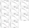Fig. A.1.

Comparison between surface brightness profiles deconvolved using the Burger – van Cittert (red solid line) and Richardson – Lucy (light blue dashed line) deconvolution techniques. Black circles show the original profile in the F814W band. The sampling (black circles) of a light profile does not correspond to the pixel scale of the WFC3 camera, but it is defined by the tool for the isophote analysis. We do not show NGC 1222. In all galaxies, the two deconvolution methods result in very comparable profiles. The differences are only seen at radii smaller than $0 \overset{″}{.} 03 - 0 \overset{″}{.} 04$ $0{{\overset{\prime\prime}{.}}}03{-}0{{\overset{\prime\prime}{.}}}04$ , which correspond to the central pixel.

The deconvolved light profiles are essentially identical on all scales. The only departure is visible in the innermost $0 \overset{″}{.} 03 - 0 \overset{″}{.} 04$ $0{{\overset{\prime\prime}{.}}}03{-}0{{\overset{\prime\prime}{.}}}04$ , which correspond to the central pixel of the WFC3 camera. Similar accuracy is claimed by Lauer et al. (1998), who used Richardson-Lucy deconvolution on WFPC2 images. Profiles deconvolved using the Richardson-Lucy method seem to achieve somewhat higher flux in the centre, but the differences are marginal, and in some cases, the deconvolution results in rougher profiles than the original data. These are dependent on the number of iterations, suggesting that this number needs to be optimised individually for each case. Nevertheless, the overall comparison clearly suggests that the Burger-van Cittert deconvolution method based on high signal-to-noise ratio HST data (and stable HST PSF), while approximate, converges, and provides sufficiently robust profiles comparable to other deconvolution techniques.

We can trust our deconvolved profiles to $\sim 0 \overset{″}{.} 04$ ${\sim}0{{\overset{\prime\prime}{.}}}04$ , therefore the question arises whether we might not also use a smaller radius to determine the slope of the inner profile. As mentioned in the paper, we wish to be consistent with the literature. Nevertheless, we calculated γ′ values for r′ = 0.05″, based on our Nuker profiles fits (Table 2). The changes in γ′ were minimal, except for NGC 0661, where the value changed from 0.96 to 0.33, and NGC 5631 where γ′ changed from 0.70 to 0.42. This means that in both cases, the classification of the light profile changed from a power-law to an intermediate, but it still remains core-less in our definition. When the same analysis is performed on the F475W images, the change for both galaxies is smaller, going to $γ_{0.05}^{'} = 0.52$ $\gamma^\prime_{0.05}=0.52$ and $γ_{0.05}^{'} = 0.59$ $\gamma^\prime_{0.05}=0.59$ for NGC 0661 and NGC 5631, respectively. The deconvolved F814W profile of NGC 5631 is worth an additional note because it seems rather flat within $0 \overset{″}{.} 7$ $0{{\overset{\prime\prime}{.}}}7$ . This is equally reproduced in the two deconvolution methods. When the F475W image is used, this is not that case and the deconvolved profiles are smoother. There is no evidence that the F814W image is saturated because our data reduction method used the shallow F814W image to substitute any saturated pixels. Even though the curvature increases for the F814W deconvolved profile, the Nuker fit returns core-less profiles, consistent with F475W profile.

Appendix B: Stellar population gradients

Table B.1.

Metallicity and age gradients for ATLAS^3D sample.

All Tables

Table 1.

General properties of the observed galaxies.

In the text

Table 2.

Parameters of the Nuker fits and kinematic structure of the analysed galaxies.

In the text

Table 3.

Incidence of kinematic and photometric features among ATLAS^3D slow rotators.

In the text

Table 4.

Median values and scatter of the metallicity gradients for the galaxies in the ATLAS^3D sample.

In the text

Table B.1.

Metallicity and age gradients for ATLAS^3D sample.

In the text

All Figures

Fig. 1.

Surface brightness profiles of the first six low-mass slow rotators from the ATLAS^3D survey (ordered by name). Each galaxy is represented by two panels. The upper panel shows light profiles in F475W (light blue squares) and F814W (red circles) filters, and the smaller lower panel shows residuals from the fit. Open symbols are original (observed) light profiles, and filled symbols are effective (deconvolved) profiles used for the analysis. The sampling does not correspond to the pixels of the WFC3 camera, but it is defined by the tool for the isophote analysis. The Nuker fits to both filters are shown with solid (F475W) and dashed (F814W) lines. Two vertical dotted lines indicate the range used in the fit. The short vertical solid line indicates the location at which the γ′ slope is measured. Our images have a pixel scale of $0 \overset{″}{.} 032$ $0{{\overset{\prime\prime}{.}}}032$ . For a comparison with Richardson-Lucy deconvolution results, see Appendix A.

In the text

Fig. 2.

Surface brightness profiles of the second six low-mass slow rotators from the ATLAS^3D survey (ordered by name). Each galaxy is represented by two panels. The upper panel shows light profiles in F475W (light blue squares) and F814W (red circles) filters, and the smaller lower panel that shows residuals from the fit. Open symbols are original (observed) light profiles, and filled symbols are effective (deconvolved) profiles used for the analysis. The sampling does not correspond to the pixels of the WFC3 camera, but is defined by the tool for the isophote analysis. The Nuker fits to both filters are shown with solid (F475W) and dashed (F814W) lines. Two vertical dotted lines indicate the range used in the fit. The short vertical solid line indicates the location at which the γ′ slope is measured. Our images have a pixel scale of $0 \overset{″}{.} 032$ $0{{\overset{\prime\prime}{.}}}032$ . For a comparison with Richardson-Lucy deconvolution results, see Appendix A.

In the text

Fig. 3.

Distribution of sizes (r_γ) and distances to core ATLAS^3D galaxies (red squares). The blue solid line shows the HST limit of r_γ < 0.1″, assumed for all galaxies that have γ′ > 0.5. Below this line, cores cannot formally be detected. Circles on the line are the upper limits on possible core sizes for galaxies presented here with values from Table 2. The histogram at the top shows the fraction of core-less galaxies in bins of distance. There is no evidence for an increase of the fraction of core-less galaxies as a result of resolution effects.

In the text

Fig. 4.

Specific stellar angular momentum vs. the observed ellipticity of the ATLAS^3D galaxies. Small open circles are galaxies with no available HST observations, and small filled circles are galaxies for which the central surface brightness profile is uncertain, mostly because of a dusty nucleus. Red diamonds are core galaxies (γ′ ≤ 0.3), and blue pentagons are core-less galaxies (γ′ > 0.3). The green solid line separates fast from slow rotators following Emsellem et al. (2011), and the grey solid line is the Cappellari (2016) alternative. The dashed magenta line shows the edge-on view for spheroidal galaxies integrated up to infinity with β = 0.7 × ϵ_intr, as in Cappellari et al. (2007). Other dashed lines show the same relation projected at inclinations of 80°, 70°, 60°, 50°, 40°, 30°, 20°, and 10° (from right to left). The dotted lines show the change in location for galaxies of intrinsic ϵ_intr = 0.85, 0.75, 0.65, 0.55, 0.45, 0.35, and 0.25 (from top to bottom). This plot differs from Fig. 4 (left) of Krajnović et al. (2013b) in that all slow rotator galaxies now have nuclear surface brightness characterisation, but the number of slow rotators with cores did not increase. NGC 1222 is the small black symbol on the grey line.

In the text

Fig. 5.

Specific stellar angular momentum vs. stellar velocity dispersion within the half-light radius for the ATLAS^3D sample. Galaxies are separated into core slow rotators, core fast rotators, core-less slow rotators, and core-less fast rotators, as shown on the legend. Galaxies with uncertain profiles and galaxies with no HST data are shown with small solid and open symbols, respectively. The box delineated by solid black lines is from Fig. 7 of Krajnović et al. (2013b), where mostly cores occur. Data presented here show that outside the box there are no new core galaxies, while the one galaxy that was previously unclassified (NGC 0661, the upper blue symbol within the box) also has a core-less surface brightness profile. The galaxy with an uncertain surface brightness profile in the box is NGC 3607, while NGC 1222 is the small solid circle with σ ∼ 90 km s⁻¹ and λ_R ∼ 0.15.

In the text

Fig. 6.

Local V/σ − h₃ diagram for slow rotators separated into core (dashed red line) and core-less (solid blue line). Contours are based on logarithmic number counts starting from 0.25 and 0.5 and then increase with a step of 0.5 until 2.5 for core slow rotators and 1.5 for core-less slow rotators, respectively. Only bins with an uncertainty δh₃ < 0.05 and σ_e > 120 km s⁻¹ are plotted. Straight lines show the slope of the distributions as measured by the ξ₃ parameter (see text for details). The inset histogram shows the distribution of the ξ₃ obtained using the jackknife method, where from the original distributions for core slow rotators and core-less slow rotators one galaxy (in each sub-sample) was randomly removed, and the ξ₃ remeasured. The histograms are notably different, with core-less slow rotators having steeper slopes (ξ₃ < 1). This confirms the robustness of the weak anti-correlation between the V/σ and h₃ distributions of core-less slow rotators.

In the text

Fig. 7.

Mass – size relations for ATLAS^3D fast (bottom) and slow (top) rotators. In both panels, small open symbols show galaxies with no HST imaging, and small filled symbols represent galaxies with uncertain light profiles. The colour specifies core (red) and core-less galaxies (light blue). Symbols refer to kinematic classes defined in Krajnović et al. (2011, see also Table 3), including KDC, CRC, 2σ, LV, NRR, and RR. Vertical lines are drawn at characteristic masses of 0.8 and 2 × 10¹¹ M_⊙. Constant velocity dispersions are shown by dashed lines. Compared to Fig. 6 of Krajnović et al. (2013b), the new HST data show that core galaxies do not appear in galaxies less massive than 0.8 × 10¹¹ M_⊙, and that all slow rotators more massive than 10¹¹ M_⊙ have cores. The black symbol in the top panel is NGC 1222.

In the text

Fig. 8.

Radial variation of metallicity profiles averaged along isophotes for all ATLAS^3D slow rotators and normalised by the half-light radii. Blue circles show metallicity profiles of slow rotators with core-less surface brightness profiles, and red squares show profiles of slow rotators with cores. Green circles belong to NGC 1222, which was not classified because of the dust. As seen in Fig. 7, core galaxies are more massive slow rotators, and the offset between the metallicity profiles of core and core-less galaxies is explained as the mass trend. Core galaxies are also larger than core-less galaxies, which explains the offsets along the horizontal axis between the two types of galaxies. The profiles differ also in their slopes, however.

In the text

Fig. 9.

Metallicity gradients vs. the stellar mass of the ATLAS^3D galaxies. Left-hand panel: all ATLAS^3D galaxies. Galaxies with cores are shown with red symbols, and core-less galaxies are represented in blue. The shape of the symbols indicates whether the galaxy is a slow (square) or a fast (circle) rotator. Diamonds show galaxies without HST imaging (empty) or with uncertain profiles (filled). NGC 1222 is shown as a green square. Red (dashed) and blue (solid) straight lines indicate the median values for core and core-less galaxies, respectively. The lengths of these lines are arbitrary and separated at mass of 10¹¹ M_⊙. The thick orange line is the running mean of Δ[Z/H]. Right-hand panel: focuses on the ATLAS^3D galaxies with HST imaging only, where coloured symbols are slow rotators, either with cores (red) or core-less (blue). Open symbols are fast rotators. Dashed lines indicate the median values for core and core-less galaxies, respectively. The thick red line is the best-fit relation for core slow rotators (red squares). Galaxies with cores tend to have shallow gradients, which flatten with the increase in mass, while core-less galaxies show a large spread.

In the text

Fig. 10.

Top: luminosity-weighted SSP α-element abundance vs. effective velocity dispersion of the ATLAS^3D galaxies. The dashed black line is the best-fit relation from McDermid et al. (2015, see their Table 5, relation i). Bottom: α-element abundance corrected for the σ_e dependance (by subtracting the values as given by the dashed line in the top panel) vs. the SSP age. Both SSP ages and [α/Fe] values are taken from McDermid et al. (2015), which also show that very old SSP ages are consistent with the fiducial age of the Universe (Planck Collaboration XIII 2016) when measurement errors and SSP mode uncertainties are taken into account. In both panels the symbols are the same and as described in the legend. Core-less slow rotators have a range of SSP ages, while core slow rotators as well as all but one core fast rotators are older than 10 Gyr.

In the text

Fig. 11.

Age gradients vs. metallicity gradient. Galaxies with cores are shown with red symbols, and core-less galaxies are represented in blue. The shape of the symbols indicates whether the galaxy is a slow (square) or a fast (circle) rotator. All galaxies follow an anti-correlation trend between the metallicity and age gradients. Core slow rotators are, however, found to have close to zero age gradients, while core-less slow rotators can have extreme positive and negative age gradients. Similar behaviour is observed for core fast rotator galaxies.

In the text

Fig. 12.

Examples of four categories of galaxies with varied stellar kinematics and nuclear surface brightness profiles. In each panel, circular symbols show the nuclear surface brightness obtained in the same way as those in Figs. 1 and 2. The solid lines represent the Nuker fits with the gradient γ′ as given in the legend. Profiles and the Nuker fits for NGC 3379, NGC 3377, and NGC 4406 (data for this galaxy are from Ferrarese et al. 2006) are taken from Krajnović et al. (2013b), while data for NGC 3522 are from the present paper. The insets show respective velocity maps, demonstrating the level of regularity and some specific kinematic structures. The colour bars show the range of velocities, which are kept the same for all galaxies for comparison. Legends also provide details on the projected ellipticity and λ_Re, taken from Emsellem et al. (2011). The two fast rotators (left column) are characterised with regular rotation. The two slow rotators (right column) exhibit a KDC (top) and a CRC (bottom). The CRC in NGC 3522 has a peak rotation of only about 20 km s⁻¹ and is located within the central 5″ (Krajnović et al. 2011).

In the text

Fig. A.1.

Comparison between surface brightness profiles deconvolved using the Burger – van Cittert (red solid line) and Richardson – Lucy (light blue dashed line) deconvolution techniques. Black circles show the original profile in the F814W band. The sampling (black circles) of a light profile does not correspond to the pixel scale of the WFC3 camera, but it is defined by the tool for the isophote analysis. We do not show NGC 1222. In all galaxies, the two deconvolution methods result in very comparable profiles. The differences are only seen at radii smaller than $0 \overset{″}{.} 03 - 0 \overset{″}{.} 04$ $0{{\overset{\prime\prime}{.}}}03{-}0{{\overset{\prime\prime}{.}}}04$ , which correspond to the central pixel.

In the text

Current usage metrics show cumulative count of Article Views (full-text article views including HTML views, PDF and ePub downloads, according to the available data) and Abstracts Views on Vision4Press platform.

Data correspond to usage on the plateform after 2015. The current usage metrics is available 48-96 hours after online publication and is updated daily on week days.

Initial download of the metrics may take a while.

[1] Algorry, D. G., Navarro, J. F., Abadi, M. G., et al. 2014, MNRAS, 437, 3596 [NASA ADS] [CrossRef] [Google Scholar]

[2] Arnold, J. A., Romanowsky, A. J., Brodie, J. P., et al. 2014, ApJ, 791, 80 [NASA ADS] [CrossRef] [Google Scholar]

[3] Bacon, R., Copin, Y., Monnet, G., et al. 2001, MNRAS, 326, 23 [NASA ADS] [CrossRef] [Google Scholar]

[4] Barnes, J. E., & Hernquist, L. E. 1991, ApJ, 370, L65 [NASA ADS] [CrossRef] [Google Scholar]

[5] Barnes, J. E., & Hernquist, L. 1996, ApJ, 471, 115 [NASA ADS] [CrossRef] [Google Scholar]

[6] Begelman, M. C., Blandford, R. D., & Rees, M. J. 1980, Nature, 287, 307 [NASA ADS] [CrossRef] [Google Scholar]

[7] Behroozi, P. S., Wechsler, R. H., & Conroy, C. 2013, ApJ, 770, 57 [NASA ADS] [CrossRef] [Google Scholar]

[8] Bellstedt, S., Forbes, D. A., Foster, C., et al. 2017, MNRAS, 467, 4540 [NASA ADS] [CrossRef] [Google Scholar]

[9] Bender, R., & Nieto, J. 1990, A&A, 239, 97 [NASA ADS] [Google Scholar]

[10] Bender, R., Saglia, R. P., & Gerhard, O. E. 1994, MNRAS, 269, 785 [NASA ADS] [CrossRef] [Google Scholar]

[11] Bendo, G. J., & Barnes, J. E. 2000, MNRAS, 316, 315 [NASA ADS] [CrossRef] [Google Scholar]

[12] Bertin, E., & Arnouts, S. 1996, A&AS, 117, 393 [NASA ADS] [CrossRef] [EDP Sciences] [Google Scholar]

[13] Bertola, F., & Capaccioli, M. 1975, ApJ, 200, 439 [NASA ADS] [CrossRef] [Google Scholar]

[14] Bezanson, R., van Dokkum, P. G., Tal, T., et al. 2009, ApJ, 697, 1290 [NASA ADS] [CrossRef] [Google Scholar]

[15] Binney, J. 1978, MNRAS, 183, 501 [NASA ADS] [Google Scholar]

[16] Binney, J. 2005, MNRAS, 363, 937 [NASA ADS] [CrossRef] [Google Scholar]

[17] Binney, J., & Tremaine, S. 2008, Galactic Dynamics, 2nd edn. (Princeton, NJ: Princeton University Press) [Google Scholar]

[18] Bois, M., Emsellem, E., Bournaud, F., et al. 2011, MNRAS, 416, 1654 (Paper VI) [NASA ADS] [CrossRef] [Google Scholar]

[19] Bonfini, P., & Graham, A. W. 2016, ApJ, 829, 81 [NASA ADS] [CrossRef] [Google Scholar]

[20] Bournaud, F., Jog, C. J., & Combes, F. 2005, A&A, 437, 69 [NASA ADS] [CrossRef] [EDP Sciences] [Google Scholar]

[21] Boylan-Kolchin, M., Ma, C.-P., & Quataert, E. 2004, ApJ, 613, L37 [NASA ADS] [CrossRef] [Google Scholar]

[22] Boylan-Kolchin, M., Ma, C.-P., & Quataert, E. 2006, MNRAS, 369, 1081 [NASA ADS] [CrossRef] [Google Scholar]

[23] Bracewell, R. N., & Roberts, J. A. 1954, Aust. J. Phys., 7, 615 [NASA ADS] [CrossRef] [Google Scholar]

[24] Brough, S., Tran, K.-V., Sharp, R. G., von der Linden, A., & Couch, W. J. 2011, MNRAS, 414, L80 [NASA ADS] [CrossRef] [Google Scholar]

[25] Brough, S., van de Sande, J., Owers, M. S., et al. 2017, ApJ, 844, 59 [NASA ADS] [CrossRef] [Google Scholar]

[26] Burger, H. C., & van Cittert, P. H. 1932, Z. Phys., 79, 722 [NASA ADS] [CrossRef] [Google Scholar]

[27] Byun, Y.-I., Grillmair, C. J., Faber, S. M., et al. 1996, AJ, 111, 1889 [NASA ADS] [CrossRef] [Google Scholar]

[28] Caon, N., Capaccioli, M., & D’Onofrio, M. 1993, MNRAS, 265, 1013 [NASA ADS] [CrossRef] [Google Scholar]

[29] Cappellari, M. 2013, ApJ, 778, L2 [NASA ADS] [CrossRef] [Google Scholar]

[30] Cappellari, M. 2016, ARA&A, 54, 597 [NASA ADS] [CrossRef] [Google Scholar]

[31] Cappellari, M., Emsellem, E., Bacon, R., et al. 2007, MNRAS, 379, 418 [NASA ADS] [CrossRef] [Google Scholar]

[32] Cappellari, M., Emsellem, E., Krajnović, D., et al. 2011a, MNRAS, 413, 813 (Paper I) [NASA ADS] [CrossRef] [Google Scholar]

[33] Cappellari, M., Emsellem, E., Krajnović, D., et al. 2011b, MNRAS, 416, 1680 (Paper VII) [NASA ADS] [CrossRef] [Google Scholar]

[34] Cappellari, M., Scott, N., Alatalo, K., et al. 2013a, MNRAS, 432, 1709 [NASA ADS] [CrossRef] [Google Scholar]

[35] Cappellari, M., McDermid, R. M., Alatalo, K., et al. 2013b, MNRAS, 432, 1862 [NASA ADS] [CrossRef] [Google Scholar]

[36] Carollo, C. M., Franx, M., Illingworth, G. D., & Forbes, D. A. 1997, ApJ, 481, 710 [NASA ADS] [CrossRef] [Google Scholar]

[37] Coccato, L., Fabricius, M., Morelli, L., et al. 2015, A&A, 581, A65 [NASA ADS] [CrossRef] [EDP Sciences] [Google Scholar]

[38] Cook, B. A., Conroy, C., Pillepich, A., Rodriguez-Gomez, V., & Hernquist, L. 2016, ApJ, 833, 158 [NASA ADS] [CrossRef] [Google Scholar]

[39] Crane, P., Stiavelli, M., King, I. R., et al. 1993, AJ, 106, 1371 [NASA ADS] [CrossRef] [Google Scholar]

[40] Crocker, A. F., Jeong, H., Komugi, S., et al. 2009, MNRAS, 393, 1255 [NASA ADS] [CrossRef] [Google Scholar]

[41] Davies, R. L., & Illingworth, G. 1983, ApJ, 266, 516 [NASA ADS] [CrossRef] [Google Scholar]

[42] Davies, R. L., Efstathiou, G., Fall, S. M., Illingworth, G., & Schechter, P. L. 1983, ApJ, 266, 41 [NASA ADS] [CrossRef] [Google Scholar]

[43] De Lucia, G., & Blaizot, J. 2007, MNRAS, 375, 2 [NASA ADS] [CrossRef] [Google Scholar]

[44] de Zeeuw, T., & Franx, M. 1991, ARA&A, 29, 239 [NASA ADS] [CrossRef] [Google Scholar]

[45] de Zeeuw, P. T., Bureau, M., Emsellem, E., et al. 2002, MNRAS, 329, 513 [NASA ADS] [CrossRef] [Google Scholar]

[46] Di Matteo, P., Pipino, A., Lehnert, M. D., Combes, F., & Semelin, B. 2009, A&A, 499, 427 [NASA ADS] [CrossRef] [EDP Sciences] [Google Scholar]

[47] D’Onofrio, M., Capaccioli, M., & Caon, N. 1994, MNRAS, 271, 523 [NASA ADS] [CrossRef] [Google Scholar]

[48] Dressler, A., & Sandage, A. 1983, ApJ, 265, 664 [NASA ADS] [CrossRef] [Google Scholar]

[49] Dubois, Y., Pichon, C., Devriendt, J., et al. 2013, MNRAS, 428, 2885 [NASA ADS] [CrossRef] [Google Scholar]

[50] Dubois, Y., Peirani, S., Pichon, C., et al. 2016, MNRAS, 463, 3948 [NASA ADS] [CrossRef] [Google Scholar]

[51] Duc, P. A., Cuillandre, J. C., Serra, P., et al. 2011, MNRAS, 417, 863 (Paper IX) [NASA ADS] [CrossRef] [Google Scholar]

[52] Dullo, B. T., & Graham, A. W. 2012, ApJ, 755, 163 [NASA ADS] [CrossRef] [Google Scholar]

[53] Dullo, B. T., & Graham, A. W. 2013, ApJ, 768, 36 [NASA ADS] [CrossRef] [Google Scholar]

[54] Dullo, B. T., & Graham, A. W. 2014, MNRAS, 444, 2700 [NASA ADS] [CrossRef] [Google Scholar]

[55] Dullo, B. T., Graham, A. W., & Knapen, J. H. 2017, MNRAS, 471, 2321 [NASA ADS] [CrossRef] [Google Scholar]

[56] Ebisuzaki, T., Makino, J., & Okumura, S. K. 1991, Nature, 354, 212 [NASA ADS] [CrossRef] [Google Scholar]

[57] Ebrová, I., & Łokas, E. L. 2017, ApJ, 850, 144 [NASA ADS] [CrossRef] [Google Scholar]

[58] Efstathiou, G., Ellis, R. S., & Carter, D. 1980, MNRAS, 193, 931 [NASA ADS] [CrossRef] [Google Scholar]

[59] Efstathiou, G., Ellis, R. S., & Carter, D. 1982, MNRAS, 201, 975 [NASA ADS] [Google Scholar]

[60] El-Zant, A. A., Freundlich, J., & Combes, F. 2016, MNRAS, 461, 1745 [NASA ADS] [CrossRef] [Google Scholar]

[61] Emsellem, E., Cappellari, M., Krajnović, D., et al. 2007, MNRAS, 379, 401 [NASA ADS] [CrossRef] [Google Scholar]

[62] Emsellem, E., Cappellari, M., Krajnović, D., et al. 2011, MNRAS, 414, 888 (Paper III) [NASA ADS] [CrossRef] [Google Scholar]

[63] Faber, S. M., Tremaine, S., Ajhar, E. A., et al. 1997, AJ, 114, 1771 [NASA ADS] [CrossRef] [Google Scholar]

[64] Fensch, J., Renaud, F., Bournaud, F., et al. 2017, MNRAS, 465, 1934 [NASA ADS] [CrossRef] [Google Scholar]

[65] Ferrarese, L., van den Bosch, F. C., Ford, H. C., Jaffe, W., & O’Connell, R. W. 1994, AJ, 108, 1598 [NASA ADS] [CrossRef] [Google Scholar]

[66] Ferrarese, L., Côté, P., Jordán, A., et al. 2006, ApJS, 164, 334 [NASA ADS] [CrossRef] [Google Scholar]

[67] Ford, H. C., Bartko, F., Bely, P. Y., et al. 1998, in Society of Photo-Optical Instrumentation Engineers (SPIE) Conference Series, eds. P. Y. Bely, & J. B. Breckinridge, 3356, 234 [NASA ADS] [Google Scholar]

[68] Foster, C., Pastorello, N., Roediger, J., et al. 2016, MNRAS, 457, 147 [NASA ADS] [CrossRef] [Google Scholar]

[69] Franx, M., Illingworth, G., & Heckman, T. 1989, ApJ, 344, 613 [NASA ADS] [CrossRef] [Google Scholar]

[70] Franx, M., Illingworth, G., & de Zeeuw, P. T. 1991, ApJ, 383, 112 [NASA ADS] [CrossRef] [Google Scholar]

[71] Frigo, M., Naab, T., Hirschmann, M., et al. 2019, MNRAS, 489, 2702 [NASA ADS] [CrossRef] [Google Scholar]

[72] Glass, L., Ferrarese, L., Côté, P., et al. 2011, ApJ, 726, 31 [NASA ADS] [CrossRef] [Google Scholar]

[73] Goddard, D., Thomas, D., Maraston, C., et al. 2017, MNRAS, 466, 4731 [NASA ADS] [Google Scholar]

[74] Goerdt, T., Moore, B., Read, J. I., & Stadel, J. 2010, ApJ, 725, 1707 [NASA ADS] [CrossRef] [Google Scholar]

[75] González Delgado, R. M., García-Benito, R., Pérez, E., et al. 2015, A&A, 581, A103 [NASA ADS] [CrossRef] [EDP Sciences] [Google Scholar]

[76] González-García, A. C., Balcells, M., & Olshevsky, V. S. 2006, MNRAS, 372, L78 [NASA ADS] [CrossRef] [Google Scholar]

[77] Graham, A. W. 2001, AJ, 121, 820 [NASA ADS] [CrossRef] [Google Scholar]

[78] Graham, A. W. 2004, ApJ, 613, L33 [NASA ADS] [CrossRef] [Google Scholar]

[79] Graham, A., Lauer, T. R., Colless, M., & Postman, M. 1996, ApJ, 465, 534 [NASA ADS] [CrossRef] [Google Scholar]

[80] Graham, A. W., Erwin, P., Trujillo, I., & Asensio Ramos, A. 2003, AJ, 125, 2951 [NASA ADS] [CrossRef] [Google Scholar]

[81] Graham, A. W., Janz, J., Penny, S. J., et al. 2017, ApJ, 840, 68 [NASA ADS] [CrossRef] [Google Scholar]

[82] Graham, M. T., Cappellari, M., Li, H., et al. 2018, MNRAS, 477, 4711 [NASA ADS] [CrossRef] [Google Scholar]

[83] Graham, M. T., Cappellari, M., Bershady, M. A., & Drory, N. 2019, A&A, submitted [arXiv:1910.05139] [Google Scholar]

[84] Greene, J. E., Leauthaud, A., Emsellem, E., et al. 2017, ApJ, 851, L33 [NASA ADS] [CrossRef] [Google Scholar]

[85] Gualandris, A., & Merritt, D. 2008, ApJ, 678, 780 [NASA ADS] [CrossRef] [Google Scholar]

[86] Gualandris, A., & Merritt, D. 2012, ApJ, 744, 74 [NASA ADS] [CrossRef] [Google Scholar]

[87] Hernquist, L. 1993, ApJ, 409, 548 [NASA ADS] [CrossRef] [Google Scholar]

[88] Hilz, M., Naab, T., Ostriker, J. P., et al. 2012, MNRAS, 425, 3119 [NASA ADS] [CrossRef] [Google Scholar]

[89] Hilz, M., Naab, T., & Ostriker, J. P. 2013, MNRAS, 429, 2924 [NASA ADS] [CrossRef] [Google Scholar]

[90] Hirschmann, M., Naab, T., Ostriker, J. P., et al. 2015, MNRAS, 449, 528 [NASA ADS] [CrossRef] [Google Scholar]

[91] Hoffman, L., Cox, T. J., Dutta, S., & Hernquist, L. 2009, ApJ, 705, 920 [NASA ADS] [CrossRef] [Google Scholar]

[92] Hoffman, L., Cox, T. J., Dutta, S., & Hernquist, L. 2010, ApJ, 723, 818 [NASA ADS] [CrossRef] [Google Scholar]

[93] Holley-Bockelmann, K., & Richstone, D. 1999, ApJ, 517, 92 [NASA ADS] [CrossRef] [Google Scholar]

[94] Hopkins, P. F., Cox, T. J., Dutta, S. N., et al. 2009a, ApJS, 181, 135 [NASA ADS] [CrossRef] [Google Scholar]

[95] Hopkins, P. F., Lauer, T. R., Cox, T. J., Hernquist, L., & Kormendy, J. 2009b, ApJS, 181, 486 [NASA ADS] [CrossRef] [Google Scholar]

[96] Hopkins, P. F., Hernquist, L., Cox, T. J., Keres, D., & Wuyts, S. 2009c, ApJ, 691, 1424 [NASA ADS] [CrossRef] [Google Scholar]

[97] Hyde, J. B., Bernardi, M., Sheth, R. K., & Nichol, R. C. 2008, MNRAS, 391, 1559 [NASA ADS] [CrossRef] [Google Scholar]

[98] Illingworth, G. 1977, ApJ, 218, L43 [NASA ADS] [CrossRef] [Google Scholar]

[99] Jedrzejewski, R. I. 1987, MNRAS, 226, 747 [Google Scholar]

[100] Jedrzejewski, R., & Schechter, P. L. 1988, ApJ, 330, L87 [NASA ADS] [CrossRef] [Google Scholar]

[101] Jedrzejewski, R., & Schechter, P. L. 1989, AJ, 98, 147 [NASA ADS] [CrossRef] [Google Scholar]

[102] Jesseit, R., Naab, T., & Burkert, A. 2005, MNRAS, 360, 1185 [NASA ADS] [CrossRef] [Google Scholar]

[103] Jesseit, R., Naab, T., Peletier, R. F., & Burkert, A. 2007, MNRAS, 376, 997 [NASA ADS] [CrossRef] [Google Scholar]

[104] Jimmy, Tran, K. V., Brough, S., et al. 2013, ApJ, 778, 171 [NASA ADS] [CrossRef] [Google Scholar]

[105] King, I. R., & Minkowski, R. 1966, ApJ, 143, 1002 [NASA ADS] [CrossRef] [Google Scholar]

[106] Kobayashi, C. 2004, MNRAS, 347, 740 [NASA ADS] [CrossRef] [Google Scholar]

[107] Koleva, M., Prugniel, P., De Rijcke, S., & Zeilinger, W. W. 2011, MNRAS, 417, 1643 [NASA ADS] [CrossRef] [Google Scholar]

[108] Kormendy, J. 1985, ApJ, 292, L9 [NASA ADS] [CrossRef] [Google Scholar]

[109] Kormendy, J., & Bender, R. 2009, ApJ, 691, L142 [NASA ADS] [CrossRef] [Google Scholar]

[110] Kormendy, J., Fisher, D. B., Cornell, M. E., & Bender, R. 2009, ApJS, 182, 216 [NASA ADS] [CrossRef] [Google Scholar]

[111] Krajnović, D., Bacon, R., Cappellari, M., et al. 2008, MNRAS, 390, 93 [NASA ADS] [CrossRef] [Google Scholar]

[112] Krajnović, D., Emsellem, E., Cappellari, M., et al. 2011, MNRAS, 414, 2923 (Paper II) [NASA ADS] [CrossRef] [Google Scholar]

[113] Krajnović, D., Alatalo, K., Blitz, L., et al. 2013a, MNRAS, 432, 1768 [NASA ADS] [CrossRef] [Google Scholar]

[114] Krajnović, D., Karick, A. M., Davies, R. L., et al. 2013b, MNRAS, 433, 2812 [NASA ADS] [CrossRef] [Google Scholar]

[115] Krajnović, D., Weilbacher, P. M., Urrutia, T., et al. 2015, MNRAS, 452, 2 [NASA ADS] [CrossRef] [Google Scholar]

[116] Krajnović, D., Emsellem, E., den Brok, M., et al. 2018a, MNRAS, 477, 5327 [NASA ADS] [CrossRef] [Google Scholar]

[117] Krajnović, D., Cappellari, M., & McDermid, R. M. 2018b, MNRAS, 473, 5237 [NASA ADS] [CrossRef] [Google Scholar]

[118] Krist, J. E., Hook, R. N., & Stoehr, F. 2011, Society of Photo-Optical Instrumentation Engineers (SPIE) Conference Series, 8127 [Google Scholar]

[119] Kulkarni, G., & Loeb, A. 2012, MNRAS, 422, 1306 [NASA ADS] [CrossRef] [Google Scholar]

[120] Kuntschner, H. 2015, in Galaxy Masses as Constraints of Formation Models, eds. M. Cappellari, & S. Courteau, IAU Symp., 311, 53 [NASA ADS] [Google Scholar]

[121] Kuntschner, H., Emsellem, E., Bacon, R., et al. 2010, MNRAS, 408, 97 [NASA ADS] [CrossRef] [Google Scholar]

[122] La Barbera, F., Ferreras, I., de Carvalho, R. R., et al. 2012, MNRAS, 426, 2300 [NASA ADS] [CrossRef] [Google Scholar]

[123] Lagos, C. D. P., Stevens, A. R. H., Bower, R. G., et al. 2018, MNRAS, 473, 4956 [NASA ADS] [CrossRef] [Google Scholar]

[124] Laine, S., van der Marel, R. P., Rossa, J., et al. 2003, AJ, 126, 2717 [NASA ADS] [CrossRef] [Google Scholar]

[125] Laporte, C. F. P., White, S. D. M., Naab, T., Ruszkowski, M., & Springel, V. 2012, MNRAS, 424, 747 [NASA ADS] [CrossRef] [Google Scholar]

[126] Lauer, T. R. 1985, ApJ, 292, 104 [NASA ADS] [CrossRef] [Google Scholar]

[127] Lauer, T. R. 2012, ApJ, 759, 64 [NASA ADS] [CrossRef] [Google Scholar]

[128] Lauer, T. R., Faber, S. M., Currie, D. G., et al. 1992, AJ, 104, 552 [NASA ADS] [CrossRef] [Google Scholar]

[129] Lauer, T. R., Ajhar, E. A., Byun, Y.-I., et al. 1995, AJ, 110, 2622 [NASA ADS] [CrossRef] [EDP Sciences] [Google Scholar]

[130] Lauer, T. R., Faber, S. M., Ajhar, E. A., Grillmair, C. J., & Scowen, P. A. 1998, AJ, 116, 2263 [NASA ADS] [CrossRef] [Google Scholar]

[131] Lauer, T. R., Faber, S. M., Gebhardt, K., et al. 2005, AJ, 129, 2138 [NASA ADS] [CrossRef] [Google Scholar]

[132] Lauer, T. R., Faber, S. M., Richstone, D., et al. 2007, ApJ, 662, 808 [NASA ADS] [CrossRef] [Google Scholar]

[133] Laurikainen, E., Salo, H., Buta, R., Knapen, J. H., & Comerón, S. 2010, MNRAS, 405, 1089 [NASA ADS] [Google Scholar]

[134] Li, H., Mao, S., Cappellari, M., et al. 2018a, MNRAS, 476, 1765 [NASA ADS] [Google Scholar]

[135] Li, H., Mao, S., Emsellem, E., et al. 2018b, MNRAS, 473, 1489 [NASA ADS] [CrossRef] [Google Scholar]

[136] Li, H., Mao, S., Cappellari, M., et al. 2018c, ApJ, 863, L19 [NASA ADS] [CrossRef] [Google Scholar]

[137] López-Cruz, O., Añorve, C., Birkinshaw, M., et al. 2014, ApJ, 795, L31 [NASA ADS] [CrossRef] [Google Scholar]

[138] Lucy, L. B. 1974, AJ, 79, 745 [NASA ADS] [CrossRef] [Google Scholar]

[139] Lynden-Bell, D. 1967, MNRAS, 136, 101 [NASA ADS] [CrossRef] [Google Scholar]

[140] Makino, J., & Ebisuzaki, T. 1996, ApJ, 465, 527 [NASA ADS] [CrossRef] [Google Scholar]

[141] Makino, J., & Funato, Y. 2004, ApJ, 602, 93 [NASA ADS] [CrossRef] [Google Scholar]

[142] Markwardt, C. B. 2009, in Astronomical Data Analysis Software and Systems XVIII, eds. D. A. Bohlender, D. Durand, & P. Dowler, ASP Conf. Ser., 411, 251 [NASA ADS] [Google Scholar]

[143] Martizzi, D., Teyssier, R., & Moore, B. 2012, MNRAS, 420, 2859 [NASA ADS] [CrossRef] [Google Scholar]

[144] Martizzi, D., Teyssier, R., & Moore, B. 2013, MNRAS, 432, 1947 [NASA ADS] [CrossRef] [Google Scholar]

[145] McDermid, R. M., Emsellem, E., Shapiro, K. L., et al. 2006, MNRAS, 373, 906 [Google Scholar]

[146] McDermid, R. M., Alatalo, K., Blitz, L., et al. 2015, MNRAS, 448, 3484 [NASA ADS] [CrossRef] [Google Scholar]

[147] Merritt, D. 2006, Rep. Prog. Phys., 69, 2513 [NASA ADS] [CrossRef] [Google Scholar]

[148] Merritt, D., & Milosavljević, M. 2005, Liv. Rev. Relativ., 8, 8 [Google Scholar]

[149] Merritt, D., Milosavljević, M., Favata, M., Hughes, S. A., & Holz, D. E. 2004, ApJ, 607, L9 [NASA ADS] [CrossRef] [Google Scholar]

[150] Merritt, D., Mikkola, S., & Szell, A. 2007, ApJ, 671, 53 [NASA ADS] [CrossRef] [Google Scholar]

[151] Mihos, J. C., & Hernquist, L. 1994, ApJ, 437, L47 [NASA ADS] [CrossRef] [Google Scholar]

[152] Milosavljević, M., & Merritt, D. 2001, ApJ, 563, 34 [NASA ADS] [CrossRef] [Google Scholar]

[153] Milosavljević, M., & Merritt, D. 2003, ApJ, 596, 860 [NASA ADS] [CrossRef] [Google Scholar]

[154] Milosavljević, M., Merritt, D., Rest, A., & van den Bosch, F. C. 2002, MNRAS, 331, L51 [NASA ADS] [CrossRef] [Google Scholar]

[155] Moody, C. E., Romanowsky, A. J., Cox, T. J., Novak, G. S., & Primack, J. R. 2014, MNRAS, 444, 1475 [NASA ADS] [CrossRef] [Google Scholar]

[156] Moré, J. J., Garbow, B. S., & Hillstrom, K. E. 1980, User Guide for MINPACK-1, Argonne National Laboratory Report ANL-80-74, 74 [Google Scholar]

[157] Moster, B. P., Naab, T., & White, S. D. M. 2013, MNRAS, 428, 3121 [NASA ADS] [CrossRef] [Google Scholar]

[158] Moster, B. P., Naab, T., & White, S. D. M. 2018, MNRAS, 477, 1822 [NASA ADS] [CrossRef] [Google Scholar]

[159] Naab, T., & Ostriker, J. P. 2017, ARA&A, 55, 59 [Google Scholar]

[160] Naab, T., Jesseit, R., & Burkert, A. 2006a, MNRAS, 372, 839 [NASA ADS] [CrossRef] [Google Scholar]

[161] Naab, T., Khochfar, S., & Burkert, A. 2006b, ApJ, 636, L81 [NASA ADS] [CrossRef] [Google Scholar]

[162] Naab, T., Johansson, P. H., Ostriker, J. P., & Efstathiou, G. 2007, ApJ, 658, 710 [NASA ADS] [CrossRef] [Google Scholar]

[163] Naab, T., Johansson, P. H., & Ostriker, J. P. 2009, ApJ, 699, L178 [NASA ADS] [CrossRef] [Google Scholar]

[164] Naab, T., Oser, L., Emsellem, E., et al. 2014, MNRAS, 444, 3357 [NASA ADS] [CrossRef] [Google Scholar]

[165] Navarro-González, J., Ricciardelli, E., Quilis, V., & Vazdekis, A. 2013, MNRAS, 436, 3507 [NASA ADS] [CrossRef] [Google Scholar]

[166] Nieto, J.-L., Bender, R., & Surma, P. 1991, A&A, 244, L37 [NASA ADS] [Google Scholar]

[167] Nipoti, C., & Binney, J. 2015, MNRAS, 446, 1820 [NASA ADS] [CrossRef] [Google Scholar]

[168] Oliva-Altamirano, P., Brough, S., Tran, K.-V., et al. 2017, AJ, 153, 89 [NASA ADS] [CrossRef] [Google Scholar]

[169] Oser, L., Ostriker, J. P., Naab, T., Johansson, P. H., & Burkert, A. 2010, ApJ, 725, 2312 [NASA ADS] [CrossRef] [Google Scholar]

[170] Pipino, A., D’Ercole, A., & Matteucci, F. 2008, A&A, 484, 679 [NASA ADS] [CrossRef] [EDP Sciences] [Google Scholar]

[171] Pipino, A., D’Ercole, A., Chiappini, C., & Matteucci, F. 2010, MNRAS, 407, 1347 [NASA ADS] [CrossRef] [Google Scholar]

[172] Planck Collaboration XIII. 2016, A&A, 594, A13 [NASA ADS] [CrossRef] [EDP Sciences] [Google Scholar]

[173] Postman, M., Lauer, T. R., Donahue, M., et al. 2012, ApJ, 756, 159 [Google Scholar]

[174] Qu, Y., Helly, J. C., Bower, R. G., et al. 2017, MNRAS, 464, 1659 [NASA ADS] [CrossRef] [Google Scholar]

[175] Quinlan, G. D. 1996, NewA, 1, 35 [NASA ADS] [CrossRef] [Google Scholar]

[176] Quinlan, G. D., & Hernquist, L. 1997, New Astron., 2, 533 [NASA ADS] [CrossRef] [Google Scholar]

[177] Quinlan, G. D., Hernquist, L., & Sigurdsson, S. 1995, ApJ, 440, 554 [NASA ADS] [CrossRef] [Google Scholar]

[178] Rantala, A., Johansson, P. H., Naab, T., Thomas, J., & Frigo, M. 2018, ApJ, 864, 113 [NASA ADS] [CrossRef] [Google Scholar]

[179] Rantala, A., Johansson, P. H., Naab, T., Thomas, J., & Frigo, M. 2019, ApJ, 872, L17 [NASA ADS] [CrossRef] [Google Scholar]

[180] Ravindranath, S., Ho, L. C., Peng, C. Y., Filippenko, A. V., & Sargent, W. L. W. 2001, AJ, 122, 653 [NASA ADS] [CrossRef] [Google Scholar]

[181] Rawle, T. D., Smith, R. J., & Lucey, J. R. 2010, MNRAS, 401, 852 [NASA ADS] [CrossRef] [Google Scholar]

[182] Renaud, F., Bournaud, F., Kraljic, K., & Duc, P. A. 2014, MNRAS, 442, L33 [NASA ADS] [CrossRef] [Google Scholar]

[183] Rest, A., van den Bosch, F. C., Jaffe, W., et al. 2001, AJ, 121, 2431 [NASA ADS] [CrossRef] [Google Scholar]

[184] Richardson, W. H. 1972, J. Opt. Soc. Am. (1917–1983), 62, 55 [Google Scholar]

[185] Richings, A. J., Uttley, P., & Körding, E. 2011, MNRAS, 415, 2158 [NASA ADS] [CrossRef] [Google Scholar]

[186] Rodriguez-Gomez, V., Pillepich, A., Sales, L. V., et al. 2016, MNRAS, 458, 2371 [NASA ADS] [CrossRef] [Google Scholar]

[187] Rothberg, B., & Joseph, R. D. 2004, AJ, 128, 2098 [Google Scholar]

[188] Rothberg, B., & Joseph, R. D. 2006, AJ, 131, 185 [NASA ADS] [CrossRef] [Google Scholar]

[189] Röttgers, B., Naab, T., & Oser, L. 2014, MNRAS, 445, 1065 [NASA ADS] [CrossRef] [Google Scholar]

[190] Rupke, D. S. N., Kewley, L. J., & Barnes, J. E. 2010, ApJ, 710, L156 [NASA ADS] [CrossRef] [Google Scholar]

[191] Rusli, S. P., Erwin, P., Saglia, R. P., et al. 2013, AJ, 146, 160 [NASA ADS] [CrossRef] [Google Scholar]

[192] Schechter, P. L., & Gunn, J. E. 1979, ApJ, 229, 472 [NASA ADS] [CrossRef] [Google Scholar]

[193] Schiavon, R. P. 2007, ApJS, 171, 146 [NASA ADS] [CrossRef] [Google Scholar]

[194] Serra, P., & Trager, S. C. 2007, MNRAS, 374, 769 [NASA ADS] [CrossRef] [Google Scholar]

[195] Serra, P., Oser, L., Krajnović, D., et al. 2014, MNRAS, 444, 3388 [NASA ADS] [CrossRef] [Google Scholar]

[196] Sérsic, J. L. 1968, Atlas de Galaxias Australes (Cordoba, Argentina: Observatorio Astronomico) [Google Scholar]

[197] Sparke, L. S., & Gallagher, III, J. S. 2000, Galaxies in the Universe: An Introduction (Cambridge, UK: Cambridge University Press) [Google Scholar]

[198] Spergel, D. N., & Hernquist, L. 1992, ApJ, 397, L75 [NASA ADS] [CrossRef] [Google Scholar]

[199] Spolaor, M., Proctor, R. N., Forbes, D. A., & Couch, W. J. 2009, ApJ, 691, L138 [NASA ADS] [CrossRef] [Google Scholar]

[200] Spolaor, M., Kobayashi, C., Forbes, D. A., Couch, W. J., & Hau, G. K. T. 2010, MNRAS, 408, 272 [NASA ADS] [CrossRef] [Google Scholar]

[201] Starkenburg, T. K., Sales, L. V., Genel, S., et al. 2019, ApJ, 878, 143 [NASA ADS] [CrossRef] [Google Scholar]

[202] Statler, T. S. 1994a, ApJ, 425, 458 [NASA ADS] [CrossRef] [Google Scholar]

[203] Statler, T. S. 1994b, ApJ, 425, 500 [NASA ADS] [CrossRef] [Google Scholar]

[204] Statler, T. S., & Fry, A. M. 1994, ApJ, 425, 481 [NASA ADS] [CrossRef] [Google Scholar]

[205] Teyssier, R., Pontzen, A., Dubois, Y., & Read, J. I. 2013, MNRAS, 429, 3068 [NASA ADS] [CrossRef] [Google Scholar]

[206] Thomas, D., Maraston, C., Bender, R., & Mendes de Oliveira, C. 2005, ApJ, 621, 673 [NASA ADS] [CrossRef] [Google Scholar]

[207] Thomas, J., Saglia, R. P., Bender, R., Erwin, P., & Fabricius, M. 2014, ApJ, 782, 39 [NASA ADS] [CrossRef] [Google Scholar]

[208] Thomas, J., Ma, C.-P., McConnell, N. J., et al. 2016, Nature, 532, 340 [NASA ADS] [CrossRef] [Google Scholar]

[209] Trujillo, I., Graham, A. W., & Caon, N. 2001, MNRAS, 326, 869 [NASA ADS] [CrossRef] [Google Scholar]

[210] Trujillo, I., Erwin, P., Asensio Ramos, A., & Graham, A. W. 2004, AJ, 127, 1917 [NASA ADS] [CrossRef] [Google Scholar]

[211] Tsatsi, A., Lyubenova, M., van de Ven, G., et al. 2017, A&A, 606, A62 [NASA ADS] [CrossRef] [EDP Sciences] [Google Scholar]

[212] van Cittert, P. H. 1931, Z. Phys., 69, 298 [NASA ADS] [CrossRef] [Google Scholar]

[213] van de Sande, J., Bland-Hawthorn, J., Fogarty, L. M. R., et al. 2017, ApJ, 835, 104 [NASA ADS] [CrossRef] [Google Scholar]

[214] van den Bosch, R. C. E. 2016, ApJ, 831, 134 [NASA ADS] [CrossRef] [Google Scholar]

[215] van der Marel, R. P., & Franx, M. 1993, ApJ, 407, 525 [NASA ADS] [CrossRef] [Google Scholar]

[216] Veale, M., Ma, C.-P., Thomas, J., et al. 2017, MNRAS, 464, 356 [NASA ADS] [CrossRef] [Google Scholar]

[217] Wellons, S., Torrey, P., Ma, C.-P., et al. 2015, MNRAS, 449, 361 [NASA ADS] [CrossRef] [Google Scholar]

[218] White, S. D. M. 1980, MNRAS, 191, 1P [NASA ADS] [CrossRef] [Google Scholar]

[219] Young, L. M., Bureau, M., Davis, T. A., et al. 2011, MNRAS, 414, 940 [NASA ADS] [CrossRef] [Google Scholar]

[220] Young, L. M., Serra, P., Krajnović, D., & Duc, P.-A. 2018, MNRAS, 477, 2741 [NASA ADS] [CrossRef] [Google Scholar]

[221] Yu, Q., & Tremaine, S. 2002, MNRAS, 335, 965 [NASA ADS] [CrossRef] [Google Scholar]

Formation channels of slowly rotating early-type galaxies⋆⋆⋆

1. Introduction

2. Data analysis

2.1. Observations

2.2. SAURON stellar populations

2.3. HST image combination

2.4. Extraction of surface brightness profiles.

3. Nuclear surface brightness profiles

3.1. Nuker profiles

3.2. Are cores of our galaxies beyond the HST resolution limit?

4. Results: not all slow rotators have cores

4.1. Cores versus rotation

4.1.1. Global kinematic parameters

4.1.2. Local kinematic parameters

4.2. Cores in the (M, Re) diagram

4.3. Metallicity gradients: evidence for different assembly processes of core and core-less galaxies

4.4. Stellar age, age gradients, and star formation histories

5. Discussion

5.1. Formation of stellar cores

5.2. Formation of flat metallicity gradients

5.3. Formation of slow rotators with and without cores

5.4. Formation of fast rotators with cores

6. Conclusions

Acknowledgments

References

Appendix A: Comparison between deconvolution methods

Appendix B: Stellar population gradients

All Tables

All Figures

Formation channels of slowly rotating early-type galaxies^⋆^⋆⋆

4.2. Cores in the (M, R_e) diagram