| Issue |
A&A
Volume 635, March 2020
|
|
|---|---|---|
| Article Number | A95 | |
| Number of page(s) | 20 | |
| Section | The Sun and the Heliosphere | |
| DOI | https://doi.org/10.1051/0004-6361/201936675 | |
| Published online | 13 March 2020 | |
Spatial scales and locality of magnetic helicity
1
Department of Mathematical Sciences, Durham University, Lower Mountjoy, Stockton Rd, Durham DH1 3LE, UK
e-mail: This email address is being protected from spambots. You need JavaScript enabled to view it.
2
Department of Mathematics, University of Exeter, N Park Rd, Exeter EX4 4QF, UK
Received:
11
September
2019
Accepted:
8
December
2019
Abstract
Context. Magnetic helicity is approximately conserved in resistive magnetohydrodynamic models. It quantifies the entanglement of the magnetic field within the plasma. The transport and removal of helicity is crucial in both dynamo development in the solar interior and active region evolution in the solar corona. This transport typically leads to highly inhomogeneous distributions of entanglement.
Aims. There exists no consistent systematic means of decomposing helicity over varying spatial scales and in localised regions. Spectral helicity decompositions can be used in periodic domains and is fruitful for the analysis of homogeneous phenomena. This paper aims to develop methods for analysing the evolution of magnetic field topology in non-homogeneous systems.
Methods. The method of multi-resolution wavelet decomposition is applied to the magnetic field. It is demonstrated how this decomposition can further be applied to various quantities associated with magnetic helicity, including the field line helicity. We use a geometrical definition of helicity, which allows these quantities to be calculated for fields with arbitrary boundary conditions.
Results. It is shown that the multi-resolution decomposition of helicity has the crucial property of local additivity. We demonstrate a general linear energy-topology conservation law, which significantly generalises the two-point correlation decomposition used in the analysis of homogeneous turbulence and periodic fields. The localisation property of the wavelet representation is shown to characterise inhomogeneous distributions, which a Fourier representation cannot. Using an analytic representation of a resistive braided field relaxation, we demonstrate a clear correlation between the variations in energy at various length scales and the variations in helicity at the same spatial scales. Its application to helicity flows in a surface flux transport model show how various contributions to the global helicity input from active region field evolution and polar field development are naturally separated by this representation.
Conclusions. The multi-resolution wavelet decomposition can be used to analyse the evolution of helicity in magnetic fields in a manner which is consistently additive. This method has the advantage over more established spectral methods in that it clearly characterises the inhomogeneous nature of helicity flows where spectral methods cannot. Further, its applicability in aperiodic models significantly increases the range of potential applications.
Key words: magnetic fields / magnetic reconnection / magnetohydrodynamics (MHD) / Sun: magnetic fields
© ESO 2020
1. Introduction
The concept of magnetic helicity for a divergence free field B is most commonly introduced as the following scalar integral quantity
 (1)
(1)
where A is the vector potential of B (B = ∇ × A). This measure was originally introduced by Woltjer (1958), and given a topological definition by Moffatt (1969) as the linking of magnetic field lines (see also Arnol’d & Khesin 1998 when field lines do not form closed curves). If we decompose a magnetic field into distinct magnetic regions (by distinct, we mean that fieldlines do not cross the boundaries of the regions within the volume V), then helicity can be decomposed into the sum of self helicities of each region, and mutual helicities between regions (Berger 1999). For example, if the regions are flux ropes, then the self helicity can be described as the twist and writhe of individual ropes, while the mutual helicity arises from the linking or braiding of distinct ropes. This decomposition has also been applied to the studies of coronal loops: see Aschwanden (2019), where the authors investigate how the stability of coronal loops is associated with the braided linking number. Other shapes are possible: for example an arcade in the solar corona can be sheared (self helicity), and it can also envelop a flux rope (mutual helicity).
Magnetic helicity is a well conserved quantity in low resistivity magnetohydrodynamics (Taylor 1974; Moffatt 2018). The conservation is maintained in less ideal conditions, albeit to a weaker degree (Berger 1984), making it an ideal approximate invariant for investigation into complex magnetic field systems (Ji et al. 1995; Brandenburg 2009; Contopoulos et al. 2009; Russell et al. 2015; Zuccarello et al. 2018).
Magnetic helicity plays an important role in studies of magnetohydrodynamic (MHD) turbulence in general, and dynamo theories of magnetic energy generation in particular (e.g. Vishniac & Cho 2001; Blackman & Brandenburg 2003; Sur et al. 2007; Brandenburg et al. 2016). In a two scale kinematic dynamo, the large scale energy can increase exponentially. This poses a problem for magnetic helicity conservation. If the large scale magnetic helicity increases exponentially, then the small scale field must have an equal and opposite helicity which also blows up. Dissipation of the small scale helicity may not be physically feasible.
A solution to this problem lies in making the dynamo inhomogeneous – the dynamo operates in one region of space (e.g. the base of the convection zone) and excess magnetic helicity is carried away (Brandenburg 2009; Vishniac & Shapovalov 2013). However, to model this process properly, we need to be able to specify how helicity is spatially distributed. In other words we need to be able to locate where helicity resides more precisely than simply using complete flux ropes.
Another area where helicity localisation could be useful is in the study of solar activity. Many studies show how magnetic helicity can flow from the interior into active regions (e.g. Berger & Ruzmaikin 2000; Kusano et al. 2002; Pevtsov 2003; Park et al. 2008; Dalmasse et al. 2014; Prior & MacTaggart 2019). A knowledge of how this helicity is distributed within the active region may aid the understanding and prediction of flares and coronal mass ejections. Scale dependence of magnetic helicity can also help in understanding the evolution of turbulence in the solar wind (Brandenburg et al. 2011).
Localising helicity is difficult for a number of reasons. First, while one can attempt to define helicity density as the quantity
 (2)
(2)
this is in no sense gauge invariant as gradient fields can be added to A without changing the magnetic field. Second, it does not represent spatially localised information, in a particular gauge such as Coulomb gauge, A is an integral over the magnetic field, and is thus non-local. This has mathematical grounding – helicity is associated with the Gauss linking number, for which we must take a double integral across all space. If we only have information about a small patch of field, there is no way of knowing how a field line goes on to twist and writhe around the rest of the field.
What about integrals of helicity as in Eq. (1)? For the expression (1) to be physically meaningful, V must either be unbounded space, or if V is finite with boundary S then S must be a either a magnetic surface  ), or the field must have periodic boundary conditions on S. If, for example, there is net flux perpendicular to two periodic directions this can lead to unphysical effects involving magnetic helicity (Berger 1997; Watson & Craig 2001; Brandenburg & Subramanian 2004).
In Sect. 2 we formally introduce the gauge problem associated with magnetic helicity, and briefly describe relative helicity, which gives a gauge-invariant measure when the volume is not bounded by a magnetic surface. In general this measure is not additive in the sense that the helicity of all space may not equal the sum of helicities of subvolumes. We then discuss Fourier decompositions of helicity, which help to provide information on how helicity behaves on various scales. Under certain circumstances (isotropic turbulence) this approach can overcome both the gauge and localisation problems; but not in the inhomogeneous aperiodic cases we would like to generalise to. This includes a discussion on the transformed two-point correlation tensor which decomposes into helicity and energy. Finally we discuss field line helicities which measure how one chosen field line interlinks with all other lines. This quantity can be used to accurately quantify reconnection activity in magnetic fields (Prior & Yeates 2018), however, the decomposition of helicity into contributions from individual fieldlines is still not localised.
In Sect. 3 we present helicity densities expressed as two-point correlation functions which are the building blocks of linking and winding. This final measure is gauge invariant, even for fields with non-trivial boundary distributions, as it does not depend on the vector potential for its definition. We select this measure as our base definition and in subsequent sections show it can be used to overcome the spatial localisation problem.
Section 4 provides a background to wavelet transforms and multi-resolution analysis as a solution to the localisation problem, and how these can be applied to helicity integrals. In Sect. 5 we give a formal introduction of the full 3D wavelet transform and its application to the helicity integral. Section 6 provides examples of how the wavelet multi-resolution helicity formulation can be applied in practice. This includes a pair of twisted flux ropes which present a trivial (null) spectral decomposition; the multi-resolution helicity decomposition is shown to resolve the spatial separation of the system’s entanglement. A second example of a pair of interlinked twisted flux ropes demonstrates how the decomposition can separate out the contributions from large scale linking and smaller scale twisting, as well as correctly assess the localisation of the helicity in this system. In Sect. 7 we consider the application of the multi-resolution wavelet decomposition to our geometric two-point correlation definition of helicity. This is used to derive linear helicity-energy decompositions for both the helicity and the field line helicity. Section 8 considers an example of a reconnecting magnetic braid, based on the numerical experiments in Wilmot-Smith et al. (2009, 2011) and Russell et al. (2015). The field line helicity multi-resolution analysis is utilised here. In particular we show that the field’s twisted structure and its field line entanglement balance their helicity fluxes at differing spatial scales. Further we show that the growth and then decay in magnetic energy of this system highly correlated with the field line helicity relaxation at that the dominant spatial scales. In Sect. 9 we apply the multi-resolution decomposition to a flux transport model and finally conclude in Sect. 10.
2. Existing helicity decompositions
2.1. The gauge problem
Suppose the volume of interest V is neither bounded by a magnetic surface or of infinite extent. This introduces a gauge dependence to the helicity integral: given some function Φ we can let AG = A + ∇Φ, which induces a change in helicity corresponding to
 (3)
(3)
To overcome this problem, Berger & Field (1984) introduced a gauge invariant measure of helicity known as “relative helicity”, which measures the magnetic helicity of the magnetic field B relative to some secondary field B0 by taking the difference between their helicities across all space. However, this quantity does not have the property of additivity; if V is decomposed into subvolumes, the relative helicity from each subvolume may not equal the total in V. Further, the reference field may not be smooth across boundaries of sub-domains.
2.2. Fourier spectra
The splitting of magnetic fields into different scales is already core to the study of many magnetohydrodynamical systems: Verma (2004) provides an in-depth review of turbulent magnetohydrodynamic fields, which have energy interchanges occurring across a spectrum of spatial scales. Following Blackman (2004, 2015), and Subramanian & Brandenburg (2005), we can write the magnetic energy spectrum as
 (4)
(4)
where k = ||k||, and a tilde represents the Fourier transform. Ωk then represents a spherical shell in wave space, given by all wavenumbers k− ≤ k ≤ k+, for which k± = ||k|| ± 0.5. In Fourier space, we have the direct relation  . Thus we can write
 (5)
(5)
and as such we have a gauge invariant measure of magnetic helicity at scale L = 2π/k which has the property of additivity (see for example Moffatt 1978; Blackman & Brandenburg 2003; Démoulin 2007; Brandenburg et al. 2016). The gauge invariance follows from the fact that the surface integral of (3) vanishes for the periodic boundary conditions required for a Fourier representation of B.
It is important to note that the Fourier decomposition can produce spurious results: if we imagine an infinite system of alternately twisted flux tubes, the Fourier transform of magnetic helicity would be zero at all scales (Asgari-Targhi & Berger 2009). To see this, suppose that Bz is constant so only has power at k = 0, but Bx and By vary in x and y to make the oppositely twisted tubes. Then at any k > 0, both k and  will be in the x − y plane. Thus the triple product must involve Bz; but Bz will be zero for k > 0.
Also the Fourier spectrum does not give information on spatial locality. The windowed Fourier transform can help. An envelope function with compact support is convolved on top of the infinite sinusoidal functions. Taking the Fourier transform using such a reduced analytic form gives an idea of the variations corresponding to scales at a given locality, but has two downsides (aside from the requirement of periodicity): firstly, the transformation does not provide an orthogonal basis, which is required to maintain additivity. Secondly, the window size is fixed, meaning we cannot separate intense fluctuations which are on smaller scales than the window size from weak contributions on the same scale as the window size.
2.3. Two-point correlation functions
An important consequence of a Fourier decomposition of a magnetic field is that the helicity Hk can be related to the magnetic energy Ek via the transform of the two-point correlation tensor Mij:
 (6)
(6)
In a periodic domain one can transform this function over the displacement x to obtain a skew-symmetric tensor function M̃ij(X,k) of both position and scale, and further, for isotropic turbulence, this can be decomposed (in three dimensions) as
![Mathematical equation: $$ \begin{aligned} \tilde{M}_{ij} = \left[ (\delta _{ij} - k^u_i k^u_j)2 E_k -\mathrm{i} k^u_l\epsilon _{ijl} k H_k \right]/8k^2 \pi , \end{aligned} $$](/articles/aa/full_html/2020/03/aa36675-19/aa36675-19-eq10.gif) (7)
(7)
where  is the ith component of the unit vector of k and ϵijl the alternating tensor (Roberts & Soward 1975; Brandenburg et al. 2016). So the energy is the trace of the tensor M̃ij and the helicity represented by the off-diagonal components. This is a potentially powerful relation between the magnetic helicity and energy on a given Fourier shell at each point of space.
In this article, we intend to provide a similar decomposition of magnetic helicity which preserves additivity and scale dependence, whilst also providing information about the spatial locality of terms contributing to the power at each scale. Key to our study is the lack of any assumptions about the boundary conditions of the magnetic fields or any isotropic assumptions. One result is a variant of (7) which can retain information on the spatial distribution of the magnetic energy and helicity, even in highly inhomogeneous systems.
2.4. Fieldline helicity
Field line helicity is another tool that has become more popular in recent years. For a given field line γ we have (Berger 1988; Yeates & Hornig 2013; Prior & Yeates 2014; Yeates & Page 2018; Moraitis et al. 2019)
 (8)
(8)
where T = B/||B|| is the unit tangent vector along the fieldline, and s is the arclength parameter of its curve. The fieldline helicity measures the average winding of all field lines around the field line under analysis (Prior & Yeates 2014). Field line helicity can be seen as the limit of the methodology of Pevtsov (2003), where each magnetic surface encloses exactly one field line. If we imagine tracing the field lines between two planes, the field line helicity associated with a field line starting at each point (xl, yl) on some initial plane (typically taken as the lower boundary of a system) gives a two-dimensional density.
The fieldline helicity is linear in A so has the property of additivity. It is not, however, gauge invariant, nor does it have the property locality as the expression for A involves an integration over at least one spatial dimension (see Prior & Yeates 2014). There is a relative field line helicity version of this quantity, whose definition comes attached with various technical complexities (Yeates & Page 2018; Moraitis et al. 2019), but is an invariant for each individual field line. Further, there is some remaining gauge dependence.
2.5. The need for a different baseline definition of helicity
These decompositions of helicity so far all have drawbacks; none combine the properties of gauge independence, spatial locality, and additivity we seek. To overcome this we begin by adopting a purely geometrical definition of helicity. We first show this has no gauge dependence, then in the following sections we show how it can be used to overcome the additivity and locality problems.
3. Magnetic winding and gauge independence
3.1. Helicity is winding
Given any integral representation for A, the helicity integral becomes a double integral involving B evaluated at two different points. For example, in Coulomb gauge with A expressed via the Biot-Savart law,
 (9)
(9)
The integrand can be regarded as a two-point correlation function for the magnetic field (Subramanian & Brandenburg 2005).
A particular topologically meaningful choice for A is the winding gauge. Prior & Yeates (2014) considered the winding gauge Aw,
 (10)
(10)
where Sz is a plane of constant z value. With this choice the helicity can be written as
 (11)
(11)
for a two-point correlation within the plane Sz of constant z. Here the set of planes Sz, z ∈ [z0, z1] cover the whole domain V. Prior & Yeates (2014) showed that (11) is just the flux-weighted average winding of all pairs of field line of B with each other, that is
 (12)
(12)
In any planar slices Sz,  , Θ(x, x′) defines the “angle” between the two fieldlines centred at x and x′,
 (13)
(13)
We demonstrate this pictorially in Fig. 1 for two curves γ and γ′. Similarly a visualisation of the topological nature of the integrand of (11), a two-point correlation function which measures the net winding, is shown in Fig. 2.
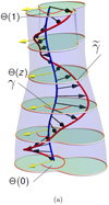 |
Fig. 1. Winding number interpretation of helicity. The winding is defined by the mutual angle Θ between two curves γ and |

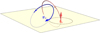 |
Fig. 2. Two point correlation interpretation of helicity. Given two field lines, the product of Bz for the first field line, and |

We remark that this requires that the field can be composed of a set of planar surfaces 𝒱 = {Sz|z ∈ [z0,z1]} and that, if the volume is finite in x or y, then the field B be tangent on the side surfaces. Berger & Hornig (2018) showed that this relation can be obtained from a poloidal-toroidal decomposition, and extended it to more general domains which can be constructed from sets of simply connected surfaces. Further it was shown in Prior & Yeates (2014) that this choice is preferable in that any other choice of gauge or reference field gives a helicity measure which is equivalent to choosing to measure the angle Θ with respect to a varying direction, whose rotation is non physical in that it does not relate to the entanglement of the field itself.
Prior & Yeates (2014) also showed that the field line helicity can be written as
 (14)
(14)
if the winding gauge is chosen. This represents the entanglement of the field line γ with the rest of the field. In Sect. 7.1 we show that, using a wavelet decomposition of B, it can be represented as a spatial sum of skew symmetric tensors whose trace give the magnetic energy and off-diagonal elements give the helicity, similar to the two-point correlation Fourier transform relationship (7).
3.2. A gauge independent measure of magnetic helicity
The crucial point about (11) is that it gives a definition of a quantity which measures the field-weighted entanglement of the magnetic field, and depends only on the field B (as does (14) for the fieldline helicity). To be sure, we can relate it to the classical magnetic helicity definition (H = ∫VA ⋅ B) via a vector potential, but the following properties can be ascribed to the quantity purely on the basis of its topological definition in terms of winding rate dΘ/dz. Firstly, it is invariant under ideal evolutions which vanish on the domain boundaries (Prior & Yeates 2014). Secondly, it is approximately conserved for low plasma β relaxations (Russell et al. 2015). Thirdly, the field line helicity density can be used to directly quantify magnetic reconnection (Prior & Yeates 2018), even for fields with normal boundary components.
These are all the properties that mark the magnetic helicity as a fundamental quantity in solar physics applications. None of them rely on a vector potential definition to be applicable (as demonstrated in the indicated references). In what follows we assert the two-point correlation function as our fundamental definition of the magnetic helicity. For the sake of clarity we formally define the following two-point correlation integral
 (15)
(15)
The product B ⋅ C represents the total winding and field weighted correlation of the field at a point (x, y) in the plane Sz with the whole field in that plane (via Eq. (11)). If the field is tangent on the boundaries of the plane Sz then C = Aw, but as we have discussed above C is a meaningful topological quantity even if this is not so.
We then have the following gauge free definitions of the helicity and field line helicity which place no requirements on the system’s boundary conditions
 (16)
(16)
 (17)
(17)
where z ∈ [0, h] is the z-coordinate which labels the set of planes Sz of the Cartesian domain on which the field is defined.
What remains is to decompose these quantities such that we have additivity and spatial locality.
4. Spatial localisation and additivity of the helicity
4.1. Localised field decompostion
Here we very briefly introduce the ideas underpinning our spatial localisation technique to give some geometrical intuition as to its interpretation. In order to spatially decompose the helicity we need a representation of the field B in terms of functions with compact support. For example the box function
 (18)
(18)
whose 3D composite
 (19)
(19)
gives a box of compact support which is translated in space. By discretizing the domain as x0 = iΔx, i ∈ 1, …N, and suitably scaling (18), a set of box functions Φlmn is created to cover the domain in a non overlapping fashion (e.g. Fig. 3a). We can then approximate the mean field B as
 (20)
(20)
 (21)
(21)
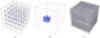 |
Fig. 3. Localised field decompositions. Panel a: a cuboid domain is split into smaller sub-boxes, which each contain a contribution to the total field, as shown in panel b. By making the discretisation even more dense, as shown in panel c, we make our approximation more accurate. |
Each coefficient Blmn is representative of the average behaviour of the field in the box (l, m, n) (Fig. 3b).
We can do something similar for the correlation integral C. Using the fact that the function Φlmn has compact support, an approximation to magnetic helicity is then given by the sum
 (22)
(22)
(think of this as a spatial decomposition of the constant part of the Fourier series). Each triplet (lmn) gives the average of the density C ⋅ B in a particular cube of the domain. To capture the local variations, we can use a function such as
 (23)
(23)
defined for all real x (such that it has compact support). The coefficients of B with respect to this function can then be added to (20) to give a more accurate approximation of the field (this is a little like breaking the sinusoid of the Fourier transform into sub components). The smaller the discretisation size (the spatial scale) N the more accurate the approximation (the discretisation in Fig. 3c would be more accurate than that in a).
Of course there are multiple issues with such a decomposition. For example how do we choose the scale of decomposition? In fact (with regards to the varying component) we might want to choose multiple scales for fields which have both large and small scale variation. How might we then add up these scales whilst avoiding redundancy? A branch of wavelet analysis called Multi-resolution Analysis tells us exactly how to perform such a decomposition orthogonally, and combine it across multiple scales. We shall introduce it formally in Sect. 5: the localised functions used above are the so-called Haar Scaling Function (18) and Haar Wavelet (23), and the sum (20) forms one part of the decomposition; the method for combining the varying field components is a little more complex. We will see in Sect. 6 that this spatial scale decomposition (multi-resolution analysis) of the helicity for the two example fields discussed above show a non trivial (absolute) variation across spatial scales which naturally identifies to “size” and position of the helicity producing components of the field.
4.2. Two-point winding correlation localisation
A decomposition such as (22) is still not fully localised, since the correlation integral C at a point (x, y, z) involves integration across planes of constant z of the domain. Thus the coefficient
 (24)
(24)
will include integration across all planes Sz containing the points (x, y, z) which have compact support from the function Φlmn. As such the quantity Clmn ⋅ Blmn represents the winding correlation of the field in the box of compact support of Φlmn with the rest of the field in the planes containing that box, as indicated in Fig. 4a.
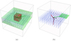 |
Fig. 4. Geometric interpretations of spatially decomposed helicity contributions. Panel a: geometrical interpretation of the spatial contribution Clmn ⋅ Blmn of a spatial (wavelet) decomposition of the helicity. The red box represents the spatial sub-domain given by the triplet lmn. Each point in this red domain contributes a winding with the rest of the field in the plane in which it is contained. Because Clmn ⋅ Blmn is a sum over the whole red domain, the set of planes containing the red domain provide winding contributions to the sum, as indicated in the figure. Panel b: winding contribution obtained by spatially decomposing the field B inside the two-point correlation function. It represents the winding of the red curve γ (localised in the plane as represented by the vector B at that point) and the field lines in the sub-plane indicated in green. |
A finer localisation can found be inserting the decomposition of the field B directly into the function C. For example, since the integral C is defined in the plane Sz we could use a two dimensional decomposition, that is use functions Φlm which approximate the field B as
 (25)
(25)
Inserting this into the field line winding integrand density (17) would yield terms in the form
 (26)
(26)
This represents the winding of the curve at the point (x, y) (represented by the vector T) with a localised sub domain of curves corresponding to the compact support of Φlm, as indicated Fig. 4b. We use this decomposition to develop a spatial helicity energy decomposition for both the helicity and field line helicity in Sect. 7. We stress that this finer decomposition requires an explicit representation of the helicity in terms of B, which our gauge free, physically, and topologically meaningful definition fulfils. This will be our ultimate solution to both the additivity and localisation problems.
5. Helicity, wavelets and multi-resolution analysis
We first consider dimensional scalar functions f(x) as 3D wavelet representations are composed of combinations of one dimensional wavelet decompositions. We will focus on the set of wavelets known as discrete wavelets which form the discrete wavelet transform, in particular the multi-resolution representation of this transform (for details on the continuous wavelet transform see e.g. Grossmann et al. 1990). What follows is far from a comprehensive overview of the mathematics the multi-resolution analysis which is beyond the scope of this study, for a more detailed introduction see, for example Farge (1992) for a practical introduction in a fluid dynamic context and Jawerth & Sweldens (1994) for more details on the underlying mathematics.
5.1. The basic idea for Haar wavelets
In the previous section we introduced the Haar Scaling function (18) and varying Haar Wavelet (23) used to characterise the mean and varying behaviour of a function f(x) respectively, over a given subset of the domain. As discussed a systematic means of choosing the and combining the domains (boxes) of compact support is required. The basic idea of a multi-resolution analysis for some function defined on a domain [0, 1] (one can always scale this to any finite domain) is to choose the domain spatial scales as factors of two 2s, …s ∈ 1, 2, …, as indicated in Table 1. Then, for a given choice of scale s the functions (23) and (18) are mutually orthogonal and orthonormal with each other if suitably dilated and translated, that is,
 (27)
(27)
 (28)
(28)
Illustrative examples of scales and locality.
A common notation for these dilation/translation combinations is to write
 (29)
(29)
so that
 (30)
(30)
One can also see some of these conditions can be extended for comparisons between scales,
 (31)
(31)
as well as
 (32)
(32)
Thus if we pick some base scale sb the orthogonality conditions (30), (31), and (32) ensure it is possible to write
 (33)
(33)
where
 (34)
(34)
for square integrable functions on [0, 1] (Jawerth & Sweldens 1994). It is a celebrated result of Ingrid Daubechies (Daubechies et al. 1993) to demonstrate that there are various classes of functions ϕ and ψ with compact support which satisfy the conditions (30), (31), (32), such that (33) can be used to represent square integrable functions. The specific choice of ϕ and ψ can often be quite important (for discussions on the matter see e.g. Farge et al. 1996; Zhang et al. 2004). The example calculations detailed in this study were performed with various wavelet choices, but no significant differences were observed, so these comparative calculations were omitted for brevity. In what follows all example calculations use the Haar basis.
In practice the series (33) will be truncated at some maximum scale sm and the most common choice is to have sb = 0, which prioritises the number of spatial scales used in the expansion, so that we have the following multi-resolution approximation:
 (35)
(35)
In what follows we use the equality sign for series such as (35) on the assumption it is understood this is actually an approximation.
The approximation (35) implies the varying behaviour of the function f on scales 2t with t > sm cannot be properly represented. More formally it can be shown that each sm yields a set of representable functions which are a subset of the square integrable functions, and further that as sm is increased each previous set of representable functions is a subset of the current set of representable functions obtained by increasing sm (Jawerth & Sweldens 1994). That is to say increasing sm will always increase the set of functions representable.
There is an analogy with the truncation of Fourier series which means one cannot represent frequencies below a given scale. This is particularly clear for the Haar wavelet. As with Fourier series truncation, the quality of representation is dependent on the degree of small scale behaviour in the function f. In practice, the target applications in solar physics would involve simulations on a numerical grid. Thus the minimum scale 2sm would be determined by the size of the grid on which the magnetic field is resolved, so the approximation would be able to resolve the same scale of function variation as the numerical grid used to resolve the field.
5.2. Three dimensional multi-resolution analysis
In a three-dimensional Cartesian domain V, we expand the function’s behaviour along each direction via a one dimensional multi-resolution expansion. We assume a 3D function H(x) can be written as Hx(x)Hy(y)Hz(z) (Jawerth & Sweldens 1994). By writing each function as a multi-resolution expansion one obtains encounter eight types of combinations (four in 2D) for each scale s:
 (36)
(36)
Writing the respective coefficients as
 (37)
(37)
the ensuing multi-resolution decomposition will be
 (38)
(38)
see for instance Farge et al. (1996).
5.2.1. Compacted notation
Throughout this study no particular attention was paid to the contributions of individual μ terms, thus for each l, m, n we shall assume the μ summation has been performed. Further, for brevity we define an index k which, when summed over will be assumed to indicate a sum over l, m and n (or just l and n in 2D). Thus we write (38) as
 (39)
(39)
5.2.2. Relative scale contributions
For a function H one can define the total (relative) contribution Qs(H) to the multi-resolution decomposition at a scale s as
 (40)
(40)
Similarly we define the relative power Ps(H) at scale s as:
 (41)
(41)
For comparison, if the function has the required periodicity we can calculate the power contained at each Fourier scale k through the quantity
 (42)
(42)
where the Hk are the coefficients of the appropriate Fourier series of H.
5.3. Helicity formulae
We consider multi-resolution expansions (39) for B (one per component) and the multi-resolution expansion of C,
 (43)
(43)
and substitute them into the helicity integral ∫V C·B dV. Using the orthogonality relationships (30), (31), and (32) we obtain a summation over the coefficients of the two series
 (44)
(44)
So Hsk is the helicity contribution at scale s at position k = lmn (summing over all directions μ). As indicated in Fig. 4a the geometrical interpretation of this coefficient corresponds to the winding of the compact domain of scale s, centred at the coordinates indicated by the triplet k, with the field in the z-slice of the volume containing this domain.
5.4. Decompositions of classical magnetic helicity
We wish to stress that the above expression (44) is equally valid for the classical definition of magnetic helicity:
 (45)
(45)
for a well-defined magnetic vector potential A. Similarly, we can define (following Finn & Antonsen 1985) a spatial decomposition of gauge-invariant relative helicity:
 (46)
(46)
where A0 and B0 are the so-called references fields, whose normal boundary components are the same as those of B and A. The physical intuition of local winding is, however, only retained when using the winding gauge Aw.
6. Multi-resolution analysis of magnetic helicity: illustrative examples
In this section we present two examples which illustrate the benefits of the spatial decomposition offered by a multi-resolution analysis of magnetic helicity. Unless otherwise stated, all quantities in this section have arbitrary units. Both examples are equally valid in either the winding correlation regime introduced here, or by using the classical definition of helicity (with the winding gauge), as the magnetic field B is tangent at the side boundaries.
6.1. Oppositely twisted flux tubes
The first of our illustrative examples is that of a pair of oppositely twisted flux tubes whose vector field takes the form
 \nonumber \\&\quad -\frac{100}{a}\exp \bigg [\frac{ -((x- 0.55)^2 + y^2)}{a^2}\bigg ](-y,x,0) + (0,0,10), \end{aligned} $$](/articles/aa/full_html/2020/03/aa36675-19/aa36675-19-eq68.gif) (47)
(47)
where we have taken a = 0.2. This field (independent of z) is visualised for the domain [−1, 1] × [−1, 1], in Fig. 5. Making an assumption of periodicity (which can be interpreted as an infinite repeating pattern of the form shown here), Fourier analysis indicates that that this magnetic field has zero overall helicity at every scale, even when the sum over k = k is taken with absolute values, as shown in Fig. 6.
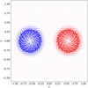 |
Fig. 5. Magnetic field vector plot of Eq. (47) at z = 0, red indicates positive twist, and blue indicates negative twist. |
By contrast, in Fig. 7, we plot the Hsk for the wavelet multi-resolution analysis of the magnetic helicity at spatial scales r = 0 → 6 (along with the associated power Ps(H)). The plotting style is that of a “bubblegram”: each sub-domain of helicity given by the multi-resolution analysis is allocated a three-dimensional sphere at its centre. The radius of this sphere is dependent upon the absolute magnitude of the helicity of the sub-domain, and its colour, red or blue, indicating a positive/negative sign respectively. In this case the magnetic field, and thus the magnetic helicity, is independent of z, but we provide the full z range as a visual indicator of the three–dimensional localising nature of wavelets.
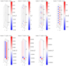 |
Fig. 7. Hsk for s = 0 → 6 applied to (47). The largest scale is a measure of the numerical round-off. At the two smallest scales 2−5, 6, the visual appearance of the bubblegram is distorted by the frequency of data points. The magnetic field and its associated helicity is independent of z. |
The bubblegrams indicate that the helicity is well localised in space in accordance with Fig. 5, presenting with the correct sign of twist. It can be seen that the total helicity Qs(H) at each scale is zero. The absolute magnetic helicity power Ps(H) is well localised in scale, as indicated in Fig. 8. Peak magnetic helicity occurs at half the spatial scale of the domain, which is in good agreement with the distribution of the twist in the magnetic field itself.
6.2. Linked rings
The magnetic helicity associated with two flux tubes, with linking number ℒ, identical individual internal twists 𝒯 and magnetic fluxes Φ is
 (48)
(48)
following Berger (1999). A simple example of such linked rings, R1 and R2 can be parametrised as
 (49)
(49)
and
 (50)
(50)
for major radius R, minor radius r ∈ [0, rm], toroidal angle θ and poloidal angle ϕ. The set Cx, Cy, Cz denote the centre of R2. An example with rm = 0.3 and R = 1 is shown in Fig. 9. We define the magnetic fields BRi of each ring as the sum of toroidal BRit and poloidal BRip components, with
 (51)
(51)
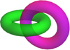 |
Fig. 9. Linked flux tubes R1 (red) and R2 (green). |
where q1 = (x2 + y2) and q2 = ((x + 1)2 + z2).
We choose R = 1 and Cx = 1, Cy = Cz = 0. Such an arrangement has an associated linking number of ℒ = 1, and we assign 𝒯 = −5, B0 = 7 and rm = 0.3, giving total magnetic helicity
 (52)
(52)
where Φ = 1.98. In Fig. 10, we plot the magnetic helicity coefficients H4k. The bubblegram indicates a distribution of magnetic helicity in correspondence to the distribution of the magnetic fields themselves, which we can attribute to the magnetic twist.
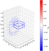 |
Fig. 10. H4k for linked tubes with 𝒯 = −5. |
In Fig. 11, we calculate the ratio of the multi-resolution expansion of helicity with that of the analytical result (from Eq. (48)) as a function of scales included, which we define by the measure
 (53)
(53)
(with and without internal magnetic twist). Naturally Ns → 1 in the limit s → ∞ as the multi-resolution analysis would be exactly the magnetic helicity. Here we see the scales at which Ns gets significantly close to 1 differ in the two cases. This is as we would expect due to the differing spatial scales between twist (small scale) and linking (large scale). We see in Fig. 12 the regions of compact support for the Haar wavelet’s at scales s = 1, 2. The s = 1 and s = 2 scales tend to cover both tubes to some degree whilst the scales s = 3 and higher generally only cover one tube. This is reflected in Fig. 11 where we see the 𝒯 = 0 field is dominated by scales s = 1, 2, as scales s = 3 and higher will reflect that on the single tube interior scale there is no complex topology. By contrast the 𝒯 = −5 case has a more balanced distribution across the scales.
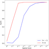 |
Fig. 11. Geometrical extent of Hsk at various scales (Haar wavelet). Panels a: s = 1 and b: s = 2 indicate the overlap of the two tubes is contained within the region of compact support. Panel c: (s = 3) the region of compact support will generally only cover one tube. |
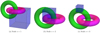 |
Fig. 12. Ns(H) calculated for two linked flux tubes. Calculations are shown with either 𝒯 = −5 (blue) or without (𝒯 = 0) internal twist (red). |
7. Helicity, energy and topology
We insert the full three-dimensional multi-resolution decomposition of the field B into the correlation function C (15) to obtain,
 (54)
(54)
where the parameter dependence of the wavelet function ψ indicates the integration is over only the in-plane functions of the 3D wavelets. In order to directly compare the helicity to the energy (helicity has an extra dimension of length) we note that if the planes Sz have x and y widths L and aL, respectively then we can write x = uL and y = avL (0 ≤ u, v ≤ 1) so that rL = L(u − u′,a(v − v′), 0), then
 (55)
(55)
where Uz is the unit square in the x–y plane. Inserting this into (16) we obtain the helicity in terms of the multi-resolution expansion of the field B alone. This calculation is most parsimoniously represented as a quadratic form, so we introduce some notation. We assume a Cartesian domain Uz × [0, h], with Uz a unit plane at height z, then the following quantities are dependent only upon the chosen wavelet, not the magnetic field itself.
 (56)
(56)
The cross-product in (54) can be represented using a skew-symmetric matrix  which takes the form
 (57)
(57)
Then, using the Einstein summation convention we have
 (58)
(58)
We note that in general the wavelet orthogonality relationships cannot be applied to (56) as the in-plane integrals are over different copies of Uz. However, the z integration is over the same domain so  will vanish if n′≠n (from the vectors k = l′m′n′ and k = lmn).
7.1. Helicity as a skew symmetric operator
We note that the helicity is being represented as a product of the field at differing positions and scales through a skew-symmetric operator M. This is analogous to the result that the helicity in periodic domains can be represented as the skew symmetric part of the Fourier transform, as discussed in Sect. 2.3. In this case we use the decomposition  , where
  (the superscript labelling is for notational convenience) is the identity matrix (one such matrix for each ss′kk′) and
 (59)
(59)
so that
 (60)
(60)
The sum of contributions to the first term for which (s′,k′) = (s, k) give the energy of the field (the multi-resolution approximation of the energy to be precise), and we can thus decompose the sum as follows
 (61)
(61)
 (62)
(62)
where δs′s is the Kronecker delta function. The operator N contains additional topological information which constitutes the helicity. In the limit which the maximum scale parameter sm (i.e. the smallest spatial scale) tends to ∞ this relationship is exact so there is a linear sum
 (63)
(63)
where N is the multi-resolution representation of a functional of the field which contains the topological information through the quantities  . A field evolution for which H is conserved requires that
 (64)
(64)
which would (approximately) apply in significantly low plasma β resistive MHD simulations.
7.2. Field line helicity
Using (16) and (55) the fieldline helicity of a field line γ at scale s and position k = lm can be written as
 (65)
(65)
where the summation over k implies a 2D multi-resolution decomposition, which is why the coefficient Bsk(z) of the multi-resolution expansion has z dependence. The contribution to 𝒜(γ) from one individual scale is then denoted 𝒜s(γ), which is then further decomposed to individual localities by 𝒜sk(γ).
Under ideal evolutions 𝒜(γ) is preserved so the sum of 𝒜s(γ) must be preserved and changes in 𝒜s(γ) must be balanced across the scales.
7.3. Helicity preserving field evolution
A particular class of fields of significant interest in the solar physics community are braided fields for which Bz > 0, ∀x ∈ V, and hence all field lines pass through the domain from the bottom to top boundary. In such cases each field lines γ can represented by the points x0 ∈ S0 where they are rooted, such that 𝒜sk(γ)≡𝒜sk(x0) and
 (66)
(66)
If the evolution is not ideal but such that the helicity is conserved (low plasma β resistive relaxations) the distribution 𝒜(γ) changes but the summation (66) must be preserved. In particular we have an alternative means of calculating the value of the operator N(B),
 (67)
(67)
The advantage is that the field line helicity representation of N is linear in both s and k so, for example, we can decompose the contributions to N as the difference H − LE at each scale s, and this decomposition is orthogonal. It is this form which we choose to utilise in this study.
8. Fieldline helicity example: analytical magnetic reconnection (the Dundee braid)
Following the resistive MHD based braiding experiments in Wilmot-Smith et al. (2009, 2011) and Russell et al. (2015) we define a field composed of exponential twist units Bt(b0, k, a, l, xc, yc, zc) given by
 (68)
(68)
where
 (69)
(69)
The parameter b0 determines the strength of the field, a the horizontal width of the twist zones, l their vertical extent, and k the handedness of the twist (k = 1 is right handed). The centre of rotation is (xc, yc, zc). The braided field is then defined as a superposition of n pairs of positive and negative twists and a uniform vertical background field
![Mathematical equation: $$ \begin{aligned} \boldsymbol{B}_{b}(1,a,l,d,z_0,s_d,n)&= \sum _{i=1}^{n}\bigg [ \boldsymbol{B}_t(1,1,a,l,-d,0,z_0+s_d(i-1)) \nonumber \\&\quad + \boldsymbol{B}_t(1,-1,a,l,0,d,0,z_0+s_d(i-1))\bigg ] + \hat{z}, \end{aligned} $$](/articles/aa/full_html/2020/03/aa36675-19/aa36675-19-eq96.gif) (70)
(70)
where d is the offset from the central axis, and sd is the vertical spacing between consecutive twists (of the same sign) and z0 the height of the first twist unit. In the literature, this is sometimes referred to as a “Dundee Braid”. By altering the extent of the twist units (the parameters a and l) one can control the overlap. The field lines in the region of overlap show significant entanglement (Fig. 13a) a property very well captured by the field line helicity distribution 𝒜(γ) (Fig. 13b). The helicity of this field is (with a suitable choice of parameters) essentially zero owing to the balance of positive and negative twisting. It was found that under a high magnetic Reynold’s number resistive MHD relaxation, under which the helicity is approximately conserved (Wilmot-Smith et al. 2011; Russell et al. 2015), that the field was able to simplify via localised reconnection into (roughly) a pair of oppositely twisted flux ropes.
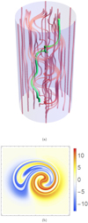 |
Fig. 13. Topological measures of (70). Panel a: subset of the field lines in the region where the fields opposing twist units overlap. The field line helicity of the green field line indicated would have contributions due to its own complex geometry as well as its entanglement with the field. Panel b: field line helicity distribution (calculated using the code used in Prior & Yeates 2018) of (71) with t = 0, there is significant small scale structure indicating the field’s complex entanglement. |
To keep matters simple in this first application of the multi-resolution decomposition 𝒜sk, we define a rough analytic approximation of this relaxation process with the following parameterised magnetic field:
 (71)
(71)
where
This field is considered in a domain x, y ∈ [−4, 4], z ∈ [−24, 24], which are the dimensions (and parameters for t = 0) used in Wilmot-Smith et al. (2009, 2011) and Russell et al. (2015). As t increases the twisted units become more and more separated in the horizontal direction, as shown in Fig. 14. The twist units (with the same sign) also merge vertically to form two non overlapping twisted flux tubes at t = 1. The decrease in overlap between the oppositely twisted units also tends to reduce the complex field entanglement (as we shall shortly see this is not true for low t). It was checked numerically that the total helicity H(B, x, y, z, t) (essentially) remains zero for all t, a property designed to approximate the numerically observed conservation of helicity in the low plasma β MHD simulations. The Fourier expansion of the magnetic helicity of this field is zero throughout (even when an absolute magnitude sum is used). In Fig. 15, we present the field line distribution of the scale decomposed field line helicity decomposition 𝒜s(x0), which involves a summation over the spatial parameter k. We remind the reader that for the field line helicity there is one such summation for each point x0 (i.e. each field line) – hence this is still a spatial distribution. The evolution of these distributions is shown at times t = 0, 0.2, 0.4, 0.6, 0.8, 0.95.
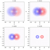 |
Fig. 14. Vector plots of (71). From top left: four time steps t = 0, 0.3, 0.6, 0.9 at z = 0. Red (blue) denotes the positively (negatively) twisted regions. |
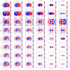 |
Fig. 15. Field line helicity distributions 𝒜s(x0) of (71). The columns from left to right represent time steps t = 0, 0.2, 0.4, 0.6, 0.8, 0.95 integrated on a domain [−4, 4]2 in x, y and [−24, 24] in z, with 400 × 400 field lines. The vertical direction indicates increasing scale s (except for the top line which is the total sum over s (it is the actual distribution 𝒜)). |
A couple of observations are worth making. Firstly, at t = 0 all scales 𝒜s(x0) show (to varying degrees) the complex mixing pattern present in the full distribution. This is a result of the field line geometry (i.e. the geometry of the green curve in Fig. 13a). Eventually this pattern disappears as the field lines reconnect and disentangle, again this is true of all scales. Secondly, there is a surrounding distribution which is most clear at the scales s = 1, 2; this persists throughout the relaxation. This is the twisted field structure of the field itself; as indicated in the twisted tube example of Sect. 6.1 twisted tube structures (which always compose the field in some manner) are dominated by contributions at these scales. Over the whole sum (over s at each t) these contributions cancel.
To quantify the entanglement variation highlighted in the first point we define a mixing parameter M as
 (72)
(72)
which will highlight the regions in which we see a rapid change in sign between positive and negative field line helicity 𝒜s(x0). Admittedly this will also capture simpler radial decay, but such contributions should be sufficiently weaker. The mixing associated with each scale, in the style of Fig. 15, is shown in Fig. 16. There are two observations. First that the mixing actually increases at first up to t = 0.4 then it decays. Second that the decay is more pronounced at larger length scales (smaller s).
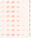 |
Fig. 16. Mixing distributions M corresponding to Fig. 15. The distributions are shown at time steps t = 0, 0.2, 0.4, 0.6, 0.8, 0.95 on a domain [−4, 4]2 in x, y and [−24, 24] in z, with 400 × 400 field lines. The vertical direction indicates increasing scale s (except for the top line which is the total sum over s (it is the actual distribution 𝒜)). |
In Fig. 17 we plot the total signed contribution per scale
 (73)
(73)
spatial integrals over the distributions shown in Fig. 14. Note that we use the Qs notation used to indicate spatial summation earlier, here it includes the spatial integration over all fieldlines, that is all x0. There is always (approximately) as much negative as positive contribution, reflecting the total helicity conservation of the field. These values are dominated by the lower scale. Their relative magnitudes increase up to about t = 0.4 then decrease over time. It is interesting that the balance of positive and negative values is always maintained by the same scales (albeit with decreasing magnitudes).
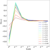 |
Fig. 17. Total fieldline helicity power QS(𝒜) attributed to each spatial scale. The distribution for s ∈ [0, 6] is shown for time periods t = 0 to t = 0.95 for the Dundee braid relaxation. |
In Fig. 18 we plot the absolute power Ps(𝒜):
 (74)
(74)
associated with each spatial scale for time steps t = 0 to t = 0.95. For early times the values (mostly) decrease with s. However, as the twisting units separate and merge the scale s = 2 becomes more prevalent, reflecting the coherent development of the twisted flux ropes. In Figs. 19 and 20 we see the total power normalised power across all scales of both the field line helicity 𝒜 and the mixing M as a function of time, given by
 (75)
(75)
Qualitatively the plots are very similar, showing a peak around 0.35 and then a relatively large drop as the twist units properly separate.
We can also directly compare the evolution of the scaled-fieldline helicity with that of magnetic energy, as shown in Fig. 21, where we plot the absolute normalised magnetic energy against that of fieldline helicity, normalised within each scale (PT(𝒜) versus PT(E)).
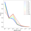 |
Fig. 18. Total fieldline helicity absolute normalised power PS(𝒜) attributed to each spatial scale. The distribution for s ∈ [0, 6] is shown for time periods t = 0 to t = 0.95 for the Dundee braid relaxation. |
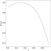 |
Fig. 19. Temporal evolution of PT(𝒜). Calculations are performed from t = 0 to t = 0.95 for the Dundee braid relaxation. |
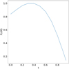 |
Fig. 20. Temporal evolution of PT(M). Calculations are performed from t = 0 to t = 0.95 for the Dundee braid relaxation. |
 |
Fig. 21. Temporal evolution of PT for 𝒜 (field line helicity) and E (magnetic energy). Each panel represents a scale s (except the first with is the total over all scales). The normalisation is scale dependent. |
The correlation between the two time series is seen to decrease as the spatial scale decreases in size. Their relative decay is most strongly aligned at scales 20 − 2−2. Whilst the decay associated with fieldline helicity power is fairly consistent at all scales, the decay of magnetic energy is opposite to that of field line helicity at scales 2−5 and 2−6. It is no surprise that the scales s = 0, 2 are the most aligned. As we see in Fig. 17 these are the dominant contributors to the field line helicity variations in the field. As the magnitude of these peaks rise (up to t = 0.3) and fall t > 0.3 (Fig. 17) so concurrently does the energy. This is a potentially important observation: that the variations in the multi-resolution decomposition of the field line helicity 𝒜sk are intimately correlated with the variations in energy in the field. In future studies it would be interesting to see whether this correlation is maintained in resistive relaxation simulations.
9. Flux of magnetic helicity
The flux of magnetic helicity through a surface is typically defined by
 (76)
(76)
for a reference field A0 (as in relative helicity) uniquely defined by the appropriate boundary conditions of magnetic field B, and velocity field v. The first term refers to dissipation within the volume, which has been shown to have an effective time scale less than energy dissipation, and we thus disregard it. The second expression can be interpreted as the sum of two individual fluxes: the effect of twisting motions on the boundary, and secondly the movement of magnetic field through the boundary.
Wavelet analysis allows us to define a fourth measure of helicity flux, giving an indication of how helicity moves spatially within the volume. An intuitive example of this could be a study of a coronal loop expanding through a simulated region, for which the twist associated with the flux rope would be seen to move spatially. multi-resolution analysis measures helicity as a set of coefficients Hsk attributed to a given scale and spatial domain (with compact support). We can then simply define
 (77)
(77)
in the form of a finite difference approximation, for the multi-resolution analyses of two adjacent time snapshots.
Further, we can perform a direct (2D) multi-resolution analysis on each term of the analytical measure of flux. For instance,
 (78)
(78)
where we note that the z-spatial co-ordinate has been dropped again (k = lm). This is a multi-resolution form of the helicity flux used in studies of the solar helicity flux through the photosphere (Hawkes & Berger 2018). Using the surface flux transport model simulations of Jiang et al. (2011), we calculate the helicity flux associated with seven spatial scales in Fig. 22 (the non-integer powers of two for the spatial scales is dependent on the resolution of the data). This data covers their simulations for Solar Cycles 21 and 22, where time is counted from the beginning of Cycle 21. As each cycle develops, the helicity flux associated with the largest scale (2−1, −2 in (cos(θ),ϕ), which equates to a hemispherical split), drops in line with an increase in helicity flux associated with Br of a smaller scale. This can be interpreted as the decreasing relative importance of polar (large scale) field relative to small-scale emerging active regions. This behaviour is seen to repeat over the course of two solar cycles (the end of the figure corresponds to the end of Cycle 22).
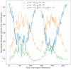 |
Fig. 22. Example Helicity flux dH/dtsk multi-resolution calculations. Equation (78) is applied to a portion of the simulations of Jiang et al. (2011). The scale 2−a, b refers to spatial scale 2−a2 in cos(θ) and 2−b2π in ϕ. Carrington rotations are counted from the beginning of Solar Cycle 21. |
10. Conclusions and future directions
10.1. Conclusions
We have demonstrated how a multi-resolution decomposition can be applied to the magnetic helicity and field line helicity, crucial topological quantities in astrophysical applications of the MHD equations. This approach is compared to spectral helicity decompositions, which require periodic domains. The method of multi-resolution analysis has some significant advantages over this purely spectral approach:
Firstly, it requires no periodicity conditions on the domain thus has a far wider range of potential applications. Secondly, it yields information on the spatial decomposition of helicity in the field. This is particularly useful for fields with significant heterogeneity of their entanglement.
On the first point the we have circumvented any issues regarding gauge choice by instead using a concrete geometrical definition of helicity. This definition combines the results of Prior & Yeates (2014) and Berger & Hornig (2018) to give a topologically meaningful definition of the helicity in terms of two–point correlation functions of B only (we need not calculate a vector potential). It has no requirements on the boundary conditions of the field to be valid. The second point is a direct consequence of decomposing the magnetic field B using a wavelet (multi-resolution) expansion, rather than a Fourier series expansion. The following explicit theoretical results were obtained.
Firstly that the helicity can be written as a sum of the components of the multi-resolution expansions of the field B and the correlation integral C, given by Eq. (44). There is an explicit geometrical interpretation of the coefficients Hsk (at scale s and position vector k) as indicated visually in Fig. 4a. We demonstrate the efficacy of this method with the multi-resolution analysis correctly identifying the opposing twisting two flux tubes in Sect. 6.1 (where the Fourier decomposition does not). In Sect. 6.2 we show there is a clear scale separation of twisting and writhing components of helicity of a pair of linked flux ropes.
Secondly, we showed it is possible to express the helicity as a linear sum:
 (79)
(79)
where the operator N is a sum over various contributions to the total winding (entanglement) of the field from the various scale and spatial components of the multi-resolution expansion of the field B, and L is the characteristic horizontal length scale of the domain. This can be seen as a significant extension of the two-point field correlation Fourier energy/helicity decomposition applicable for fields in periodic domains (see e.g. Brandenburg et al. 2016). This decomposition not only places no requirement on the boundary conditions of the field but also gives information about the spatial distribution of contributions to this sum.
Thirdly it was shown that the field line helicity 𝒜(γ), the average entanglement of the field line γ with the rest of the field, can be composed into both spatial and scale components using a multi-resolution analysis (see Eq. (65)). Under an ideal evolution, when the distribution of field line helicity is conserved, this decomposition could be used to provide insight as to how the field’s topology redistributes both spatially and across scales (e.g. flux ropes kinking/expanding or buoyantly rising through the convection zone of the sun). In this initial study we applied the field line helicity decomposition to an analytic representation of a resistively relaxing magnetic braid whose total helicity is conserved (mimicking well known numerical experiments of low plasma β resistive MHD relaxation of the same magnetic braid configuration Russell et al. 2015). In this case the spatially integrated sum of the field line helicity at each scale, which is equal to the helicity and hence conserved, indicated that the conservation was maintained by a varying balance of entanglement on scales which reflected the varying field line entanglement and the twisted structure of the underlying magnetic field. It was also seen that the variance in these contributions strongly correlated with the variations in energy of the field during its relaxation.
Finally, we demonstrated how to apply this multi-resolution decomposition to helicity fluxes through a planar boundary. An example application of this to a surface flux transport model over two solar cycles is used to indicate the varying contributions from the large-scale polar field and the smaller scale active regions.
In addition to these results and findings we have developed a number of simple methods/quantities which can be used to draw conclusions from the expansions, such as the scale total and power coefficients Qs and Ps, and the mixing measure M used to interpret the varying degree of complexity of the field line helicity decompositions in Sect. 8.
10.2. Future directions
The next step of this study would be to apply these techniques to Resistive MHD simulations. Based on the results of this study, we propose that the following lines of inquiry should be a priority.
Firstly, it is known that there is a clear relationship between the Fourier energy and helicity spectrum in homogeneously driven turbulence (e.g. Brandenburg et al. 2016). The question to answer is whether there is a similar relationship in highly heterogeneous systems for a multi-resolution decomposition of the energy and helicity. The energy scale/field line helicity scale correlation, found in the analytically driven braid relaxation of Sect. 8 offers some promise, but it should be investigated as to whether this same behaviour manifests in the resistive MHD relaxations of Wilmot-Smith et al. (2009, 2011) and Russell et al. (2015).
Secondly, what information can be obtained from the helicity energy decomposition? In particular, under a field evolution which preserves helicity, the product represented by the operator N must oppose that of the energy. Further, N contains the topological information of the field. Since this decomposition applies at each spatial point of a discretised field an in-depth analysis of the transfer between these two quantities may be able to yield information as to how reconnection activity can lead to a field relaxing to force free equilibrium. Of particular interest will be simulations which do not follow the Taylor relaxation hypothesis (those which relax to a non-linear force free equilibrium), as they imply the assumption that the helicity is the only topological quantity not destroyed during relaxation is not true in general.
Thirdly, can the decomposition be used to identify relatively large spatial scale substructure in heterogeneous turbulence? For example partial flux rope type structures. Finally, does the decomposition, applied to flux transport type simulations or magnetogram data indicate anything about the variations in behaviour of solar cycles?
Acknowledgments
We thank the UK STFC for their funding under grants ST/N504063/1 (GH) and ST/R000891/1 (MAB). This collaboration was facilitated through the NORDITA programme on Solar Helicities in Theory and Observations. The authors would also like to thank the anonymous referee for their helpful comments which greatly improved both the quality and clarity of this work.
References
- Arnol’d, V., & Khesin, B. 1998, Topological Magnetohydrodynamics (Berlin: Springer) [CrossRef] [Google Scholar]
- Aschwanden, M. J. 2019, ApJ, 874, 131 [NASA ADS] [CrossRef] [Google Scholar]
- Asgari-Targhi, M., & Berger, M. A. 2009, Geophys. Astrophys. Fluid Dyn., 103, 69 [NASA ADS] [CrossRef] [Google Scholar]
- Berger, M. A. 1984, Geophys. Astrophys. Fluid Dyn., 30, 79 [NASA ADS] [CrossRef] [Google Scholar]
- Berger, M. 1988, A&A, 201, 355 [NASA ADS] [Google Scholar]
- Berger, M. A. 1997, J. Geophys. Res., 102, 2637 [NASA ADS] [CrossRef] [Google Scholar]
- Berger, M. A. 1999, Plasma Phys., 41, 167 [Google Scholar]
- Berger, M. A., & Field, G. B. 1984, J. Fluid Mech., 147, 133 [NASA ADS] [CrossRef] [Google Scholar]
- Berger, M. A., & Hornig, G. 2018, J. Phys. A: Math. Theoret., 51, 495501 [Google Scholar]
- Berger, M. A., & Ruzmaikin, A. 2000, J. Geophys. Res.: Space Phys., 105, 10481 [NASA ADS] [CrossRef] [Google Scholar]
- Blackman, E. G. 2004, Plasma Phys. Control. Fusion, 46, 423 [NASA ADS] [CrossRef] [Google Scholar]
- Blackman, E. G. 2015, Magnetic Helicity and Large Scale Magnetic Fields: A Primer (Dordrecht: Springer Science+Business Media), 188, 59 [Google Scholar]
- Blackman, E. G., & Brandenburg, A. 2003, ApJ, 584, L99 [NASA ADS] [CrossRef] [Google Scholar]
- Brandenburg, A. 2009, Plasma Phys. Control. Fusion, 51, 124043 [NASA ADS] [CrossRef] [Google Scholar]
- Brandenburg, A., & Subramanian, K. 2004, Phys. Rep., 141, 1502 [Google Scholar]
- Brandenburg, A., Subramanian, K., Balogh, A., & Goldstein, M. 2011, ApJ, 734, 9 [NASA ADS] [CrossRef] [Google Scholar]
- Brandenburg, A., Petrie, G. J. D., & Singh, N. K. 2016, ApJ, 836, 21 [Google Scholar]
- Contopoulos, I., Christodoulou, D. M., Kazanas, D., & Gabuzda, D. C. 2009, ApJ, 702, L148 [NASA ADS] [CrossRef] [Google Scholar]
- Dalmasse, K., Pariat, E., Démoulin, P., & Aulanier, G. 2014, Sol. Phys., 289, 107 [NASA ADS] [CrossRef] [Google Scholar]
- Daubechies, I., Meyer, Y., Lemerie-Rieusset, P. G., et al. 1993, Different Perspectives on Wavelets, 47, 1 [CrossRef] [Google Scholar]
- Démoulin, P. 2007, AdSpR, 39, 1674 [NASA ADS] [CrossRef] [Google Scholar]
- Farge, M. 1992, Ann. Rev. Fluid Mech., 24, 395 [NASA ADS] [CrossRef] [Google Scholar]
- Farge, M., Kevlahan, N., Perrier, V., & Goirand, E. 1996, Proc. IEEE, 84, 639 [CrossRef] [Google Scholar]
- Finn, J., & Antonsen, T. M. 1985, Plasma Phys. Control. Fusion., 111, 111 [Google Scholar]
- Grossmann, A., Kronland-Martinet, R., & Morlet, J. 1990, Wavelets (Berlin: Springer), 2 [CrossRef] [Google Scholar]
- Hawkes, G., & Berger, M. A. 2018, Sol. Phys., 293, 109 [Google Scholar]
- Jawerth, B., & Sweldens, W. 1994, SIAM Rev., 36, 377 [CrossRef] [Google Scholar]
- Ji, H., Prager, S. C., & Sarff, J. 1995, Phys. Rev. Lett., 74, 2945 [NASA ADS] [CrossRef] [Google Scholar]
- Jiang, J., Cameron, R. H., Schmitt, D., & Schüssler, M. 2011, A&A, 528, A82 [NASA ADS] [CrossRef] [EDP Sciences] [Google Scholar]
- Kusano, K., Maeshiro, T., Yokoyama, T., & Sakurai, T. 2002, ApJ, 577, 501 [NASA ADS] [CrossRef] [Google Scholar]
- Moffatt, H. K. 1969, J. Fluid. Mech., 35, 117 [Google Scholar]
- Moffatt, H. 1978, Magnetic Field Generation in Electrically Conducting Fluids (Cambridge: Cambridge University Press) [Google Scholar]
- Moffatt, H. K. 2018, Comptes Rendus - Mecanique, 346, 165 [NASA ADS] [CrossRef] [Google Scholar]
- Moraitis, K., Pariat, E., Valori, G., & Dalmasse, K. 2019, A&A, 624, A51 [NASA ADS] [CrossRef] [EDP Sciences] [Google Scholar]
- Park, S.-H., Lee, J., Choe, G.-S., et al. 2008, ApJ, 686, 1397 [NASA ADS] [CrossRef] [Google Scholar]
- Pevtsov, A. A. 2003, ApJ, 593, 1217 [NASA ADS] [CrossRef] [Google Scholar]
- Prior, C., & MacTaggart, D. 2019, J. Plasma Phys., 85, 775850201 [CrossRef] [Google Scholar]
- Prior, C., & Yeates, A. 2014, ApJ, 787, 100 [Google Scholar]
- Prior, C., & Yeates, A. R. 2018, Phys. Rev. E, 98, 013204 [NASA ADS] [CrossRef] [Google Scholar]
- Roberts, P., & Soward, A. 1975, Astron. Nachr., 296, 49 [NASA ADS] [CrossRef] [Google Scholar]
- Russell, A. J., Yeates, A. R., Hornig, G., & Wilmot-Smith, A. L. 2015, Phys. Plasmas, 22, 032106 [NASA ADS] [CrossRef] [Google Scholar]
- Subramanian, K., & Brandenburg, A. 2005, ApJ, 648, L71 [NASA ADS] [CrossRef] [Google Scholar]
- Sur, S., Shukurov, A., & Subramanian, K. 2007, MNRAS, 377, 874 [NASA ADS] [CrossRef] [Google Scholar]
- Taylor, J. B. 1974, Phys. Rev. Lett., 33, 1139 [NASA ADS] [CrossRef] [Google Scholar]
- Verma, M. K. 2004, Phys. Rep., 401, 229 [NASA ADS] [CrossRef] [Google Scholar]
- Vishniac, E. T., & Cho, J. 2001, ApJ, 550, 752 [NASA ADS] [CrossRef] [Google Scholar]
- Vishniac, E. T., & Shapovalov, D. 2013, ApJ, 780, 144 [NASA ADS] [CrossRef] [Google Scholar]
- Watson, P., & Craig, I. 2001, J. Geophys. Res. Space Phys., 106, 15735 [NASA ADS] [CrossRef] [Google Scholar]
- Wilmot-Smith, A., Hornig, G., & Pontin, D. 2009, ApJ, 704, 1288 [NASA ADS] [CrossRef] [Google Scholar]
- Wilmot-Smith, A., Pontin, D., Yeates, A., & Hornig, G. 2011, A&A, 536, A67 [NASA ADS] [CrossRef] [EDP Sciences] [Google Scholar]
- Woltjer, L. 1958, Proc. Natl. Acad. Sci., 44, 489 [NASA ADS] [CrossRef] [Google Scholar]
- Yeates, A., & Hornig, G. 2013, Phys. Plasmas, 20, 012102 [NASA ADS] [CrossRef] [Google Scholar]
- Yeates, A. R., & Page, M. H. 2018, J. Plasma Phys., 84, 775840602 [CrossRef] [Google Scholar]
- Zhang, T., Sun, H., & Wu, P. 2004, Flow Measurement Instrum., 15, 325 [CrossRef] [Google Scholar]
- Zuccarello, F. P., Pariat, E., Valori, G., & Linan, L. 2018, ApJ, 863, 41 [Google Scholar]
All Tables
All Figures
|
Fig. 1. Winding number interpretation of helicity. The winding is defined by the mutual angle Θ between two curves γ and |
| In the text | |
|
Fig. 2. Two point correlation interpretation of helicity. Given two field lines, the product of Bz for the first field line, and |
| In the text | |
|
Fig. 3. Localised field decompositions. Panel a: a cuboid domain is split into smaller sub-boxes, which each contain a contribution to the total field, as shown in panel b. By making the discretisation even more dense, as shown in panel c, we make our approximation more accurate. |
| In the text | |
|
Fig. 4. Geometric interpretations of spatially decomposed helicity contributions. Panel a: geometrical interpretation of the spatial contribution Clmn ⋅ Blmn of a spatial (wavelet) decomposition of the helicity. The red box represents the spatial sub-domain given by the triplet lmn. Each point in this red domain contributes a winding with the rest of the field in the plane in which it is contained. Because Clmn ⋅ Blmn is a sum over the whole red domain, the set of planes containing the red domain provide winding contributions to the sum, as indicated in the figure. Panel b: winding contribution obtained by spatially decomposing the field B inside the two-point correlation function. It represents the winding of the red curve γ (localised in the plane as represented by the vector B at that point) and the field lines in the sub-plane indicated in green. |
| In the text | |
|
Fig. 5. Magnetic field vector plot of Eq. (47) at z = 0, red indicates positive twist, and blue indicates negative twist. |
| In the text | |
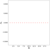 |
Fig. 6. Fourier decomposition Hk of magnetic helicity for the field (47). |
| In the text | |
|
Fig. 7. Hsk for s = 0 → 6 applied to (47). The largest scale is a measure of the numerical round-off. At the two smallest scales 2−5, 6, the visual appearance of the bubblegram is distorted by the frequency of data points. The magnetic field and its associated helicity is independent of z. |
| In the text | |
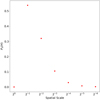 |
Fig. 8. Ps(H) for s = 0 → 6 applied to (47). |
| In the text | |
|
Fig. 9. Linked flux tubes R1 (red) and R2 (green). |
| In the text | |
|
Fig. 10. H4k for linked tubes with 𝒯 = −5. |
| In the text | |
|
Fig. 11. Geometrical extent of Hsk at various scales (Haar wavelet). Panels a: s = 1 and b: s = 2 indicate the overlap of the two tubes is contained within the region of compact support. Panel c: (s = 3) the region of compact support will generally only cover one tube. |
| In the text | |
|
Fig. 12. Ns(H) calculated for two linked flux tubes. Calculations are shown with either 𝒯 = −5 (blue) or without (𝒯 = 0) internal twist (red). |
| In the text | |
|
Fig. 13. Topological measures of (70). Panel a: subset of the field lines in the region where the fields opposing twist units overlap. The field line helicity of the green field line indicated would have contributions due to its own complex geometry as well as its entanglement with the field. Panel b: field line helicity distribution (calculated using the code used in Prior & Yeates 2018) of (71) with t = 0, there is significant small scale structure indicating the field’s complex entanglement. |
| In the text | |
|
Fig. 14. Vector plots of (71). From top left: four time steps t = 0, 0.3, 0.6, 0.9 at z = 0. Red (blue) denotes the positively (negatively) twisted regions. |
| In the text | |
|
Fig. 15. Field line helicity distributions 𝒜s(x0) of (71). The columns from left to right represent time steps t = 0, 0.2, 0.4, 0.6, 0.8, 0.95 integrated on a domain [−4, 4]2 in x, y and [−24, 24] in z, with 400 × 400 field lines. The vertical direction indicates increasing scale s (except for the top line which is the total sum over s (it is the actual distribution 𝒜)). |
| In the text | |
|
Fig. 16. Mixing distributions M corresponding to Fig. 15. The distributions are shown at time steps t = 0, 0.2, 0.4, 0.6, 0.8, 0.95 on a domain [−4, 4]2 in x, y and [−24, 24] in z, with 400 × 400 field lines. The vertical direction indicates increasing scale s (except for the top line which is the total sum over s (it is the actual distribution 𝒜)). |
| In the text | |
|
Fig. 17. Total fieldline helicity power QS(𝒜) attributed to each spatial scale. The distribution for s ∈ [0, 6] is shown for time periods t = 0 to t = 0.95 for the Dundee braid relaxation. |
| In the text | |
|
Fig. 18. Total fieldline helicity absolute normalised power PS(𝒜) attributed to each spatial scale. The distribution for s ∈ [0, 6] is shown for time periods t = 0 to t = 0.95 for the Dundee braid relaxation. |
| In the text | |
|
Fig. 19. Temporal evolution of PT(𝒜). Calculations are performed from t = 0 to t = 0.95 for the Dundee braid relaxation. |
| In the text | |
|
Fig. 20. Temporal evolution of PT(M). Calculations are performed from t = 0 to t = 0.95 for the Dundee braid relaxation. |
| In the text | |
|
Fig. 21. Temporal evolution of PT for 𝒜 (field line helicity) and E (magnetic energy). Each panel represents a scale s (except the first with is the total over all scales). The normalisation is scale dependent. |
| In the text | |
|
Fig. 22. Example Helicity flux dH/dtsk multi-resolution calculations. Equation (78) is applied to a portion of the simulations of Jiang et al. (2011). The scale 2−a, b refers to spatial scale 2−a2 in cos(θ) and 2−b2π in ϕ. Carrington rotations are counted from the beginning of Solar Cycle 21. |
| In the text | |
Current usage metrics show cumulative count of Article Views (full-text article views including HTML views, PDF and ePub downloads, according to the available data) and Abstracts Views on Vision4Press platform.
Data correspond to usage on the plateform after 2015. The current usage metrics is available 48-96 hours after online publication and is updated daily on week days.
Initial download of the metrics may take a while.