| Issue |
A&A
Volume 635, March 2020
|
|
|---|---|---|
| Article Number | A39 | |
| Number of page(s) | 22 | |
| Section | Interstellar and circumstellar matter | |
| DOI | https://doi.org/10.1051/0004-6361/201936553 | |
| Published online | 04 March 2020 | |
The long-lived Type IIn SN 2015da: Infrared echoes and strong interaction within an extended massive shell★,★★
1
Department of Astronomy and the Oskar Klein Centre, Stockholm University,
AlbaNova, Roslagstullsbacken 21,
114 21
Stockholm,
Sweden
e-mail: This email address is being protected from spambots. You need JavaScript enabled to view it.
2
INAF – Osservatorio Astronomico di Padova,
Vicolo dell’Osservatorio 5,
35122
Padova,
Italy
3
Tuorla Observatory, Department of Physics and Astronomy, 20014, University of Turku,
Turku,
Finland
4
School of Physics, O’Brien Centre for Science North, University College Dublin,
Belfield Dublin 4,
Ireland
5
Department of Applied Physics, Universidad de Cádiz,
campus of Puerto Real,
11510
Cádiz,
Spain
6
Institute of Space Sciences (ICE, CSIC), Campus UAB,
Camí de Can Magrans s/n,
08193,
Cerdanyola del Vallès,
Barcelona,
Spain
7
Institut d’Estudis Espacials de Catalunya (IEEC),
c/Gran Capità 2–4, Edif. Nexus 201,
08034
Barcelona,
Spain
8
Benoziyo Center for Astrophysics and the Helen Kimmel center for planetary science, Weizmann Institute of Science,
76100
Rehovot,
Israel
9
Xinjiang Astronomical Observatory,
150 Science 1–Street,
Urumqi,
Xinjiang
830011,
PR China
10
Xingming Observatory,
Mountain Nanshan, Urumqi,
Xinjiang 830011,
PR China
11
Graduate Institute of Astronomy, National Central University,
300 Zhongda Rd., Zhongli District, Taoyuan City
32001,
Taiwan,
PR China
12
Department of Astronomy/Steward Observatory,
933 North Cherry Avenue, Rm. N204,
Tucson,
AZ 85721-0065,
USA
13
Osservatorio Astronomico di Monte Agliale,
Via Cune Motrone,
55023
Borgo a Mozzano,
Lucca,
Italy
14
Physics Department and Tsinghua Center for Astrophysics, Tsinghua University,
Beijing
100084,
PR China
15
Yunnan Observatories, Chinese Academy of Sciences,
Kunming
650216,
PR China
16
Key Laboratory for the Structure and Evolution of Celestial Objects, Chinese Academy of Sciences,
Kunming
650216,
PR China
17
Department of Astronomy, School of Physics and Astronomy, Shanghai Jiaotong Univeristy,
Shanghai
200240,
PR China
18
Key Laboratory of Optical Astronomy, National Astronomical Observatories, Chinese Academy of Sciences,
10101
Beijing,
PR China
19
School of Astronomy and Space Science, University of Chinese Academy of Sciences,
101408
Beijing,
PR China
20
Center for Astrophysics | Harvard & Smithsonian,
60 Garden Street,
Cambridge,
MA
02138-1516,
USA
21
Las Cumbres Observatory,
6740 Cortona Drive, Suite 102,
Goleta,
CA
93117-5575,
USA
22
Department of Physics, University of California,
Santa Barbara,
CA
93106-9530,
USA
23
Department of Physics, University of California,
Davis,
CA
95616,
USA
24
The Oskar Klein Centre, Physics Department, Stockholm University,
AlbaNova, Roslagstullsbacken 21,
21 Stockholm,
Sweden
25
Division of Physics, Mathematics and Astronomy, California Institute of Technology,
Pasadena,
CA
91125,
USA
26
Space Telescope Science Institute,
3700 San Martin Drive,
Baltimore,
MD
21218,
USA
27
European Southern Observatory Karl – Schwarzschild – Str 2 85748,
Garching bei München,
Germany
28
Center for Interdisciplinary Exploration and Research in Astrophysics (CIERA) and Department of Physics and Astronomy, Northwestern University,
Evanston,
IL
60208,
USA
Received:
22
August
2019
Accepted:
29
December
2019
Abstract
In this paper we report the results of the first ~four years of spectroscopic and photometric monitoring of the Type IIn supernova SN 2015da (also known as PSN J13522411+3941286, or iPTF16tu). The supernova exploded in the nearby spiral galaxy NGC 5337 in a relatively highly extinguished environment. The transient showed prominent narrow Balmer lines in emission at all times and a slow rise to maximum in all bands. In addition, early observations performed by amateur astronomers give a very well-constrained explosion epoch. The observables are consistent with continuous interaction between the supernova ejecta and a dense and extended H-rich circumstellar medium. The presence of such an extended and dense medium is difficult to reconcile with standard stellar evolution models, since the metallicity at the position of SN 2015da seems to be slightly subsolar. Interaction is likely the mechanism powering the light curve, as confirmed by the analysis of the pseudo bolometric light curve, which gives a total radiated energy ≳ 1051 erg. Modeling the light curve in the context of a supernova shock breakout through a dense circumstellar medium allowed us to infer the mass of the prexisting gas to be ≃ 8 M⊙, with an extreme mass-loss rate for the progenitor star ≃0.6 M⊙ yr−1, suggesting that most of the circumstellar gas was produced during multiple eruptive events. Near- and mid-infrared observations reveal a fluxexcess in these domains, similar to those observed in SN 2010jl and other interacting transients, likely due to preexisting radiatively heated dust surrounding the supernova. By modeling the infrared excess, we infer a mass ≳ 0.4 × 10⁻³ M⊙ for the dust.
Key words: supernovae: general / galaxies: individual: NGC 5337 / supernovae: individual: PSN J13522411+3941286 / supernovae: individual: iPTF16tu / supernovae: individual: SN 2015da
Tables A.1–A.4 are only available at the CDS via anonymous ftp to cdsarc.u-strasbg.fr (130.79.128.5) or via http://cdsarc.u-strasbg.fr/viz-bin/cat/J/A+A/635/A39.
Spectroscopic data and photometric tables are available through the Weizmann Interactive Supernova Data Repository (WISeREP) at the following address: https://wiserep.weizmann.ac.il/object/13868.
© ESO 2020
1 Introduction
Supernovae (SNe) interacting with a preexisting dense circumstellar medium (CSM) belong to an intriguing and not fully understood class of transients, including the Ibn (Pastorello et al. 2008) and IIn (Schlegel 1990) classes. Early optical spectra of Type IIn SNe show a blue continuum with narrow (from a few tens to ≃103 km s−1) Balmer lines in emission, and broad wings resulting from electron scattering in an ionized, unshocked, H-rich CSM (see, e.g., Chugai 2001). These lines, visible at all phases of the spectroscopic evolution, are the signature of underlying interaction between SN ejecta and slow moving CSM, as they are the result of recombination in the outer unshocked layers, ionized by photons emitted in the shocked regions. When the fast-moving ejecta hit the preexisting CSM, forward/reverse shocks form at the interface between the two media (also producing a contact discontinuity and a “cool dense shell” – CDS; Fransson 1984; Chevalier & Fransson 1994), and high energy photons propagate in both directions, either ionizing the freely expanding SN ejecta or the slow-moving CSM.
Under specific conditions (e.g., particular geometrical configurations), the resulting emission lines can be characterized by structured, asymmetric, and multicomponent profiles, produced by recombining gas shells moving at different velocities (see, e.g., the case of the prototypical SNe 1987F; Wegner & Swanson 1996 and 1988Z; Stathakis & Sadler 1991; Turatto et al. 1993), although in other cases, the overall profiles are characterized by pure Lorentzian profiles at all epochs (see, e.g., the case of SN 2010jl; Fransson et al. 2014). Depending on the density of the CSM, the early light curve of IIn SNe might be dominated by photon diffusion rather than 56Ni decay (e.g., Balberg & Loeb 2011), possibly extending the “shock breakout” signal (e.g., Ofek et al. 2010; Chevalier & Irwin 2011). Modeling the bolometric light curves of SNe exploding in a dense wind allows us to infer crucial information about the nature of the exploding star and its environment (such as the mass-loss rate and the mass of the surrounding CSM; e.g., Balberg & Loeb 2011; Svirski et al. 2012). Narrow lines, if resolved, may also be used to infer wind speeds directly from their P Cygni absorption features.
Type IIn SNe are relatively rare (~9% of all Type II, H-rich core-collapse SNe – CC SNe; Li et al. 2011), although they are more common than Ibn SNe. They show a remarkable heterogeneity, with absolute peak magnitudes ranging from Mr = −17 to − 22 mag (Kiewe et al. 2012; Taddia et al. 2013b), with a mean rise time of ≃17 d (based on the sample of 15 objects published in Ofek et al. 2014a). On the other hand, this value might be strongly affected by the limited number of SNe IIn discovered soon after explosion and/or well-studied transients, whose publication is likely biased towards the most peculiar or luminous objects (see, e.g., SN 2006gy; Ofek et al. 2007; Smith et al. 2007, and the “super-luminous” Type II SNe – SLSN II; Gal-Yam 2019). A recent analysis on a greater sample of 42 SNe IIn discovered by the Palomar Transient Factory (PTF) reveals an average peak luminosity of Mr = −19.18 ± 1.32 mag and a bimodal distribution of rise times, with trise = 19 ± 8 d and 50 ± 15 d (Nyholm et al. 2020). A wide range of photometric properties is also observed after peak, with a fraction of IIn SNe (e.g., SNe 1988Z; Stathakis & Sadler 1991; Turatto et al. 1993, 2005ip and 2006jd; Stritzinger et al. 2012) showing a very slow evolution, with the transient still visible several years after explosion (see, e.g., SN 1995N; Fransson et al. 2002; Pastorello et al. 2005). In other cases, light curves exhibit a plateau-like shape with steep post-plateau declines (IIn-P; Kankare et al. 2012; Mauerhan et al. 2013) or otherwise almost “linear” declines (see, e.g., the case of SN 1999el; Di Carlo et al. 2002). Long-lasting Type IIn SNe are generally brighter than IIn-P, although not as bright as SLSNe.
The controversy surrounding the nature of the progenitors of SNe IIn is still not completely solved. The presence of an extended and dense CSM at the time of the explosion requires strong long-term winds, binary interactions, or giant eruptive events similar to those occasionally experienced by luminous blue variables (LBVs; Vink 2012, and references therein). Some observational evidence points to LBVs as progenitors of at least some Type IIn SNe. The direct observation of the likely quiescent progenitors of SNe 2005gl (Gal-Yam & Leonard 2009) and 2009ip (Smith et al. 2010) in deep archival Hubble Space Telescope (HST) images strongly supports this scenario, as well as the disappearance of the LBV candidate progenitor of SN 2005gl in a post-explosion HST image obtained when the SN had faded (Gal-Yam & Leonard 2009). Nevertheless, pre-SN super-winds might not be rare in red supergiant (RSG) stars (see, e.g., the case of the Galactic RSG VY Canis Majoris; Smith et al. 2009a) suggesting that they are viable progenitors for at least a fraction of SNe IIn (as proposed for SN 1995N; Fransson et al. 2002; Pozzo et al. 2004). In addition, Tartaglia et al. (2016) showed that also stars less massive than LBVs can experience major eruptive events. Some observational evidences seem to suggest thermonuclear explosions of stars embedded in a dense and extended CSM as viable mechanisms to produce some Type IIn SNe. These Ia-CSM SNe (see, e.g., Silverman et al. 2013; Fox et al. 2015a) show optical spectra dominated by prominent narrow Balmer lines in emission and luminosities usually exceeding those typically observed in normal SNe Ia. A number of transients have been proposed to belong to this class (see, e.g., Silverman et al. 2013), although their real nature is still a matter of discussion (see, e.g., Benetti et al. 2006; Trundle et al. 2008; Inserra et al. 2016). On the other hand, the analysis performed on high-resolution optical spectra of PTF11kx (Dilday et al. 2012) revealed features first resembling those of the overluminous Type Ia SN 1999aa (see, e.g., Garavini et al. 2004, and references therein), but soon developing strong narrow Hα features, therefore suggesting that a fraction of SNe showing narrow emission features arise from thermonuclear explosions.
More than 50% of SNe showing late (or very late, see, e.g., SNe 1999el; Di Carlo et al. 2002 and 2005ip; Fox et al. 2009, 2010, among others) infrared (IR) excess belong to the IIn class (see Gerardy et al. 2002; Fox et al. 2011), although this percentage might be biased by the still limited number of well studied SNe IIn in the IR domain. This suggests the presence of either preexisting or newly formed dust. Dust can, in fact, form in the rapidly cooling post-shock layers (e.g., Pozzo et al. 2004; Mattila et al. 2008) or be located in the dense preexisting CSM, becoming visible after being shock- or radiatively heated, or because echoing and reprocessing some of the SN light into IR radiation (e.g., Fox et al. 2010; Stritzinger et al. 2012; Fransson et al. 2014). Modeling the IR emission of SNe IIn showing late-time excesses can independently infer crucial information on the environments of progenitor stars as well as their mass-loss rates (e.g., Fox et al. 2010).
In this context, we report the results of our study of the long-lasting Type IIn SN 2015da. The SN was discovered on 2015 January 9.90 UT in the nearby spiral galaxy NGC 5337 by Z. Jin and X. Gao1, with an apparent magnitude ≃18 mag, and was later classified as a Type IIn SN (Zhang & Wang 2015). No source was detected at the position of the transient in an unfiltered image obtained on 2015 January 7 to a limiting magnitude 19.5 mag, or in previous frames of the field. SN 2015da is located at RA = 13:52:24.11, Dec = +39:41:28.2 [J2000], 12.′′ 54 E, 14.′′ 04 N from the center of NGC 5337 (assuming RA = 13:52:23.024, Dec = + 39:41:14.16 – J2000 – for the center of the host; Skrutskie et al. 2006, see also Fig. 1). The SN was extensively imaged by amateur astronomers, who provided very good sampling of the rise to the maximum through unfiltered images, later calibrated to the R-band. SN 2015da was also followed by a number of facilities and collaborations, such as the Nordic Optical Telescope Un-biased Transient Survey (NUTS2) and its extension NUTS2, and the intermediate Palomar Transient Facility3 (iPTF) under the designation of iPTF16tu. The discovery of SN 2015da was also reported by Petropoulou et al. (2017), who estimated a distance of 32.1 Mpc based on the redshift derived from the heliocentric recessional velocity of NGC 5337 (2165 ± 17 km s−1; van Driel et al. 2001), and a cosmology with ΩM = 0.31, ΩΛ = 0.69, and H0 = 69.9 km s−1 Mpc−1.
The paper is organized as follows: Sect. 2 describes the host galaxy, metallicity, and star formation rate at the location of SN 2015da, including a discussion on the local reddening. In Sect. 3, we report our analysis on data collected during the photometric (Sect. 3.1) and spectroscopic (Sect. 3.2) follow-up campaigns, and give a qualitative interpretation of the observed quantities. A summary of the main results of the paper is reported in Sect. 4, while in the appendix, we detail the observations and data-reduction techniques, provide the magnitude tables, and main information on the spectra.
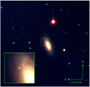 |
Fig. 1 Combined gri images of the field of NGC 5337 obtained on 2019 January 23 with the Nordic Optical Telescope with ALFOSC. The position of SN 2015da, still clearly visible, is highlighted within a green box. The insert shows SN 2015da, which is the bright source within the zoomed-in region. |
2 The host galaxy and local extinction
NGC 5337 is a SBab galaxy, with a total corrected4 apparent B-band magnitude of 12.94 ± 0.29 mag and mean heliocentric radial velocity (cz) Vr = 2127 ± 2 km s−1 (as reported in the HyperLeda database5). In the following, we assume a luminosity distance of 53.2 ± 13.2 Mpc (corresponding to a distance modulus of 33.63 ± 0.54 mag), which is the most recent redshift–independent distance estimate for NGC 5337 (Tully et al. 2016). We note, however, a large discrepancy among different distances reported in the literature for NGC 5337 (in particular among redshift-dependent distances reported in the NASA/IPAC Extragalactic Database – NED6). Assuming a distance modulus μ = 33.63 ± 0.54 mag implies a total absolute magnitude of B = −20.69 ± 0.61 mag. The main properties inferred for SN 2015da and its environment described in this section are reported in Table 1.
An estimate of the local metallicity in the environment of SN 2015da can be inferred through the analysis of the spectral emission lines of a relatively nearby H II region, SDSS J135223.63+394136.2, located at RA = 13:52:23.63, Dec = +39:41:36.21 [J2000] (i.e., 5.′′ 54 W, 8.′′ 01 N from the position of SN 2015da, corresponding to a projected distance of 2.51 kpc at 53.2 Mpc). The spectrum of the H II region, available through the Sloan Digital Sky Survey Data Release 14 (SDSS DR14; Adelman-McCarthy et al. 2006) was obtained through the SDSS Catalog Archive Server (CAS7). After correcting the spectrum for the foreground Galactic extinction, we estimated the internal reddening through the observed Balmer decrement, assuming an intrinsic ratio of 2.86 (case B recombination scenario, see Osterbrock & Ferland 2006) and a standard extinction law with RV = 3.1 (Cardelli et al. 1989). Following Botticella et al. (2012), we therefore corrected the spectrum of the H II region by including an additional contributionof E(B−V) = 0.47 mag to the total color excess.
The local metallicity in the environment of the H II region was inferred from the integrated flux ratios of the diagnostic lines Hα and [N II]λ6583. Following Pettini & Pagel (2004) and using their recalibration of the N2 ≡ log([N II]λ6583∕Hα) index (Denicoló et al. 2002), we get 12 + log[O/H] = 8.45 dex from their linear relation, and 8.39 dex using their third-order polynomial fit (their Eqs. (1) and (2), respectively). We could not use other emission line diagnostics (such as O3N2; Alloin et al. 1979) since we did not detect the required lines for these methods (i.e., [O III] λ4363 or λ5007). Since it is well established that peripheral H II regions have lower metallicities than those closer to the galactic centers, we then used metallicity gradients available in the literature to infer an estimate of the local oxygen abundance at the position of SN 2015da with respect to the value inferred at the position of the H II region. We computed the de-projected normalized distances (rSN ∕R25 and rHII ∕R25) from the center of NGC 5337 following Hakobyan et al. (2009, their Eqs. (1) and (2); see also Taddia et al. 2013a). Using the coordinates of the SN and the host center, the inclination and major axis position angle (PA) reported in the HyperLeda database, we inferred de-projected distances rSN∕R25 = 0.35 and rHII∕R25 = 0.47 (17.′′ 38 and 23.′′ 65 offset from the center of NGC 5337) for the SN and the H II region, respectively. Assuming a metallicity gradient of − 0.47 R∕R25 (i.e., the average of the metallicity gradients reported in Pilyugin et al. 2004, for a sample of galaxies), we extrapolated the oxygen abundance at the galactocentric distance of SN 2015da, obtaining an averaged nearly solar value of 12 + log[O/H] = 8.48 dex (assuming a solar metallicity of 12 + log[O/H] = 8.69 dex; Asplund et al. 2009). Although affected by the assumption on the metallicity gradient and by the fact that line diagnostic methods are generally believed to underestimate local abundances (see, e.g., López-Sánchez et al. 2012), this result is in agreement with the one reported by Taddia et al. (2015) on a sample of interacting SNe, showing that long-lasting SNe IIn, like SN 2015da, seem to occur in marginally subsolar metallicity environments.
The host galaxy extinction was estimated as detailed below. From the DEIMOS spectrum, we inferred an equivalent width (EW) of 1.3 and 1.2 Å for the D2 and D1 lines of the Na ID doublet, respectively, which are both above the linearity range of the relation between the Na I D EW and E(B−V) (≃ 0.6Å; see Poznanski et al. 2012). This suggests a highly extinguished environment. We therefore used different methods to estimate the local extinction. Although Type IIn SNe show a remarkable heterogeneity, we notice a strong similarity between the spectroscopic and photometric evolutions of SN 2015da and SN 2010jl (e.g., Stoll et al. 2011; Zhang et al. 2012; Fransson et al. 2014; Borish et al. 2015, see Sect. 3). On the basis of this similarity, we used the available data to infer an estimate of the extinction, fitting the evolution of the spectral continuum of SN 2015da to that of SN 2010jl. Since Type IIn SNe typically show prominent Balmer lines in emission, we compared the evolution of the temperature of the pseudo photosphere estimated fitting black-body (BB) functions to selected regions of the spectral continuum (i.e., those not affected by the presence of strong emission lines, like Hα or Hβ). We therefore fitted the temperatures using a standard extinction law (assuming RV = 3.1; Cardelli et al. 1989) within the first ≃200 d from the R-band maximum (in this context, we refer to the R-band maximum, since the explosion epoch of SN 2010jl is not well constrained). For each epoch, we let the V -band extinction vary within the AV = 0−4 mag range with steps of 0.08 mag, considering the one minimizing the χ2 distributions derived at each epoch as the best fit model. With this method, we obtain E(B−V) ≃ 0.97 ± 0.10 mag for RV = 3.1 (assuming a conservative 10% error due to the uncertainty in the flux calibration of the spectra), whereas we do not notice a significant improvement (although we get a slightly higher extinction) when allowing RV to vary within the 2−4 range (see Fig. 2). A similar approach is to consider the evolution of the spectral energy distribution (SED) computed using those bands typically unaffected by the presence of strong emission lines, which, therefore, map the shape of the spectral continuum (BV IHK) more closely. Following the prescriptions of Tartaglia et al. (2018) (see also Elias-Rosa et al. 2006, for an equivalent approach), we fitted the evolution of the SED of SN 2015da to that of SN 2010jl (computed using the same bands), finding a good agreement with the previous result, obtaining E(B−V) ≃ 0.92 ± 0.10 mag.
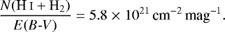
In order to test the robustness of these estimates, we compared this value with that obtained using an alternative method, based on the presence of particular features in sufficiently high-resolution spectra of highly extinguished SNe. While we do not notice any strong evidence of diffuse interstellar bands (DIBs; see, e.g., Herbig 1995; Sollerman et al. 2005) in the DEIMOS spectrum, we inferred an independent estimate of the local extinction by fitting the strong Na ID features using the Voigt profile fitting VPFIT8 code (and RV = 3.1), convolving theoretical Voigt line profiles with the spectral resolution to fit the observed features, therefore obtaining an Na I column density of logNNa = 13.53 ± 0.08 dex. Following Ferlet et al. (1985) we used the relation:
![Mathematical equation: \begin{equation*} \log{N(\textrm{Na\,I})=1.04[\log{N(\textrm{H\,I}+\textrm{H}_2)}]-9.09}, \end{equation*}](/articles/aa/full_html/2020/03/aa36553-19/aa36553-19-eq1.png) (1)
(1)
(with N(Na I) and N(H) in cm−2) to infer the neutral hydrogen column density and thus compute an estimate of the color excess through the relation given by Bohlin et al. (1978):
 (2)
(2)
Using these prescriptions, we get an additional color excess due to the extinction in the SN environment of E(B−V) = 0.96 ± 0.27 mag, which is in agreement with the estimates reported above. Therefore, in the following, we use E(B−V) ≃ 0.97 mag (assuming a standard extinction law with RV = 3.1) as the host galaxy reddening, implying a total color excess of E(B−V) = 0.98 ± 0.30 mag (accounting for the uncertainties of the different methods used above) in the direction of SN 2015da.
Summary of the main properties of SN 2015da and its environment.
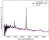 |
Fig. 2 Fit to the continuum of the optical spectrum obtained at + 56 d after R-band maximumcompared to a spectrum of the Type IIn SN 2010jl at a similar phase. The fit wasobtained by varying the amount of the extinction for SN 2015da in order to have aBB temperature comparable with that computed for SN 2010jl. We first fixed RV = 3.1 and then let it vary within the RV = 2−4 range. |
3 Analysis and discussion
In the following, we qualitatively discuss the main results of the analysis on the available photometric and spectroscopic data. In-depth modeling and focused analysis are to be the subject of a forthcoming paper.
3.1 Photometry
Optical, near- and mid-IR (NIR and MIR, respectively) light curves of SN 2015da are shown in Figs. 3 and 4, respectively, and the apparent magnitudes are reported in Tables A.1–A.4 (available through the CDS), along with apparent magnitudes of the local standard stars used for the photometric calibration (Table A.5). Optical and NIR photometric data were mainly obtained using the telescopes of the Las Cumbres Observatory9 network (Brown et al. 2013) within the Supernova Key Project and by the NUTS collaboration10.
To estimate the explosion epoch, we first fitted a power law to the early R-band light curve (the one with the best coverage of the rise time including the latest nondetection limit) at tMJD ≤ 57122 (i.e. ≃ 90 d after the discovery). This choice is based on the shape of the R-band light curve during the rise, which is well-reproduced by a power law at early phases only. Performing 104 Monte Carlo (MC) simulations randomly shifting the data points within their errors, we find that the early R-band light curve of SN 2015da evolves as  , suggesting an explosion epoch roughly coincident with the discovery. On the other hand, given the large uncertainties surrounding the early points, we prefer to take the midpoint between the discovery and the lastnondetection as a more conservative estimate, therefore assuming 2015 January 8.45 UT (JD=2457030.945, ≃ 1.45 d before the first detection) as the explosion epoch of SN 2015da. Rise times in different bands were computed in the same way, fitting high-order polynomials to the light curves through MC simulations. We find slow rise times in all bands, increasing from the blue (trise,U = 35 ± 10 d) to the red bands (trise,R,I = 100 ± 5 d), with the longest period found in the NIR bands (106 ± 10, 110 ± 10, and 126 ± 10 d in J, H, and K-band, respectively), resulting in bright absolute magnitudes at peak (e.g., MR = −20.45 ± 0.55 and MI = −20.39 ± 0.55 mag; see Table 2). Errors on the absolute magnitudes are dominated by the large uncertainty in the distance to NGC 5337. In Fig. 5, we show that the resulting R-band peak magnitude is consistent with that of SN 2010jl (Fransson et al. 2014), also showing many other features comparable to those observed in SN 2015da (see below and Sect. 3.2).
The R-band light curve is the one with the best coverage thanks to the well-cadenced early observations provided by the amateurs. During the first ~ 26 d, it shows a relatively fast rise at a rate of 0.2 mag d−1, followed by a flattening in the light curve with a rate decreasing to ≃0.06 mag d−1 in the remaining 74 d before maximum. Only a handful of Type IIn SNe have rises with such good coverage and well-estimated explosion epochs (see, e.g., the samples discussed in Ofek et al. 2014a and Nyholm et al. 2020). A good sampling of the peak was also obtained in V and I, where we notice similar slow rises (0.005 mag d−1 and 0.009 mag d−1) at + 21 ≲ t ≲ +100 d. After peak, the R-band light curve shows a first rapid decline, withthe luminosity getting ≃0.5 mag fainter in ~65 d, and then it flattens at a rate of 0.004 mag d−1. At ≃+400 d, the slope slightly increases to 0.005 mag d−1 until ≃ + 700 d, when we note a further flattening, with the exception of the U∕u bands, where the light curves show linear declines after peak (0.003 mag d−1 and 0.008 mag d−1 in u and U, respectively,where the discrepancy can be attributed to the larger scatter in the U-band light curve).We notice a similar behavior in the other optical bands.
The relatively bright peak magnitudes of SN 2015da are comparable to the brighter end of the distribution presented in Nyholm et al. (2020) (see also Silverman et al. 2013, for a preliminary analysis on PTF SNe IIn), extending the range of luminosities inferred by Kiewe et al. (2012) to slightly higher values. The rise times observed in SN 2015da, on the other hand, seem to fall way outside the range found for their sample of 42 Type IIn SNe, although a similar (but still ~ 40 d shorter) rise was also observed in the overluminous Type IIn SN 2006gy (Ofek et al. 2007; Smith et al. 2007; Fox et al. 2015b; Agnoletto et al. 2009, see Fig. 5, right panel). An explanation for the lack of very long-lasting SNe IIn might be the still low number of early discoveries for this type of transient, for which some progress has been made to drastically increase the quality of the data in samples, yet it might still significantly affect statistical studies.
NIR light curves evolve in a similar way up to ≃+400 d, where we notice a rebrightening, more pronounced in the K-band, lasting ≃ 240 d with an increase of ≃1 mag. In order to collect the most complete information possible, we searched for NEOWISE Reactivation Survey detections of SN 2015da in the W1 (3.4 μm) and W2 (4.6 μm) bands. The first detection of a source at the SN position occured during the pass of June 2015 (18–25), 162 d after the explosion (see Table A.4). No detections were recorded during the previous pass occurred a few days before the SN explosion (25–31 Dec. 2014), for which we only obtained upper limits (W1 > 15.7 mag and W2 > 15.3 mag). Since then, the SN was detected at all passings, with a cadence of approximately six months in both bands (Table A.4) showing a similar evolution with respect to the NIR bands (see Fig. 4).
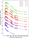 |
Fig. 3 Optical light curves of SN 2015da during the first ≃4 yr after the explosion. Magnitudes are calibrated in the Vega (UBV RI) and AB systems (ugriz) and are not corrected for the MW or host galaxy extinction. |
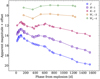 |
Fig. 4 IR light curves of SN 2015da during the first ≃4 yr after the explosion. Magnitudes are calibrated in the Vega system. |
Rise times and absolute peak magnitudes of SN 2015da in optical and NIR bands.
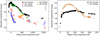 |
Fig. 5 Left: comparison of the R-band light curve of SN 2015da with those of SNe 1988Z (Turatto et al. 1993), 2005ip, 2006jl (Stritzinger et al. 2012) and 2010jl (Fransson et al. 2014). Absolute magnitudes were obtained using Milky Way and host galaxy extinctions and adopting distances reported in the literature. The representative error barcorresponds to the uncertainty on the distance of NGC 5337. Right: comparison of the R-band light curve of SN 2015da with that of the overluminous SN 2006gy up to ≃ 250 d. |
3.1.1 Evolution of the spectral energy distribution and analysis of the near infrared excess
In order to model the excess in the IR luminosity observed at t ≳ 400 d, we analyzed the evolution of the SED of SN 2015da from t = +33 d to + 1233 d with a regular interval of 50 d. This choice is based on the available photometric points (e.g., the first available u-band point is at + 33 d). Apparent magnitudes were interpolated at each epochs, corrected for the total extinction as estimated in Sect. 2, and converted in flux using the appropriate effective wavelengths and zero points available in the literature for each band. Effective wavelengths were corrected for the heliocentric recessional velocity inferred from the narrow Na ID features in absorption (see Sect. 3.2). Figure 6 shows the results of the fit at selected epochs, reported in Table 3.
We used BB functions (using a single, or a combination of two BBs, when appropriate) to fit the SED evolution, excluding u-band fluxes at t ≥ +83 d and bands bluer than R at t ≥ +183 d, since strong blends of Fe II lines start to dominate the blue spectral continuum around this epoch, and the SED can no longer be approximated by a BB at λ ≲ 5500Å. On the other hand, we estimated the contributions of Hα and Pa γ lines in order to remove them from the integrated fluxes in the r, R and J bands. Since the integrated flux of Pa γ could be directly estimated from the spectra only at two epochs (i.e., + 26 d and + 606 d), we linearly interpolated its contributionto the J-band at the desired epochs, while the evolution of Hα was estimated with higher accuracy (see Sect. 3.2.2). Similarly, to avoid extrapolation, we did not include MIR fluxes at t < +183 d.
The SEDs were modeled following Suzuki & Fukugita (2018, see their Eqs. (1) and (2)) through a Markov chain Monte Carlo (MCMC11) routine based on the PYTHON EMCEE package, using the following expression:
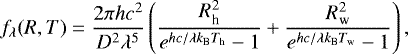 (3)
(3)
where Rh, Th, Rw, and Tw are the radii and temperatures of the hot and warm components, respectively, and D is the distance to SN 2015da. Adopting a luminosity distance of 53.2 ± 13.2 Mpc (see Sects. 1 and 2), we could therefore infer the radii of the two emitting regions, assuming pure thermal emission at the equilibrium temperatures Th and Tw and spherical symmetry. A more detailed analysis, including geometrical considerations (such as the one performed by Andrews et al. 2011, for SN 2010jl), is beyond the scope of this paper and is to be presented in a forthcoming paper. Up to + 433 d, the SED is well-reproduced using a single BB with a temperature decreasing from 12 700 ± 150 K to 5850 ± 90 K. During the same period, the radius of the photospheric component increases from (1.81 ± 0.02) × 1015 to (3.49 ± 0.07) × 1015 cm in the first 150 d, and then decreases during the following 500 d (see Table 3).
From + 433 d, we need a second BB to properly reproduce the SED, showing a slightly decreasing temperature (after an initial increase from 1280 ± 40 K to 1510 ± 20 K, probably due to a residual contamination from the photospheric component) and a BB radius increasing from (2.06 ± 0.10) × 1016 to (2.60 ± 0.05) × 1016 cm. At later times (t ≥ +733 d), the fit to the IR flux is well-reproduced by a single warm component with slightly decreasing temperatures (from 1400 to 1000 K, see Table 3). This suggests a negligible contribution of the photospheric component in the IR domain and the absence of an additional cooler component at these epochs.
IR excesses are more common in long-lasting Type IIn SNe at late times (t ≳100 d) than in other SN types (e.g., Fox et al. 2011) and are generally interpreted as thermal emission from either preexisting or newly formed dust (see, e.g., Gerardy et al. 2002; Mattila et al. 2008). To get a rough estimate of the mass of dust needed to produce the observed excess, we followed the prescriptions of Fox et al. (2010), fitting the following expression to the observed SEDs:
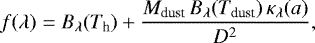 (4)
(4)
where Bλ(Th) is the BB resulting from the hot component (from Eq. (3)), Mdust is the total mass of the dust, Bλ(Tdust) the BB at the temperatureof the dust, Tdust, κλ (a) the mass absorption coefficient for a dust particle of radius a as derived fromMie theory, and D is the distance of the emitting source to the observer. This formalism assumes only thermal emission at the equilibrium temperature Td and dust composed entirely either of carbon- or oxygen-rich grains (graphite and silicates, respectively) of a single size. Following Stritzinger et al. (2012), we fitted the model to the observed SEDs using dust grains of three sizes (0.01, 0.1, and 1 μm, see Table 4), fixing Th, Rh to the values derived from Eq. (3) (Table 3). For s = 0.1 μm, at + 1233 d we get ≃ 5 and 10 × 10−3 M⊙ of preexisting dust in the CSM for graphite and silicates, respectively. As a comparison, for the same size of graphite grains, Fox et al. (2013) found masses in the 2 × 10⁻⁵−3 × 10⁻² M⊙ range for their sample of SNe IIn with available Spitzer data, so the masses inferred using Eq. (4) for SN 2015da are compatible with their derived values. Assuming a standard gas-to-dust ratio of 1 : 100, this indicates a CSM mass of 0.5−1M⊙ for SN 2015da, which is similar to that inferred by Fox et al. (2013) for SN 2010jl (1− 2M⊙ taking the gas-to-dust ratio computed by Mauron & Josselin 2011). On the other hand, in Sect. 3.1.2 we find a much higher value of swept up CSM (≃ 8M⊙). This difference could be due to the assumptions made when estimating the dust mass (such as grain sizes), composition, and geometrical configuration. More accurate models are necessary to infer the physical properties of the dust producing the IR excess observed in SN 2015da.
We note that BB radii inferred for the IR component (Table 3) are similar to those derived for the dust evaporation radius in SN 2010jl by Fransson et al. (2014) for large graphite grains. This would seem to favor large graphite grains as the main components of the preexisting dust. On the other hand, since we do not have access to MIR spectra, we cannot rule out silicates or graphite as the main composition for the dust grains. The highest Td we infer fitting Eq. (3) (≃1510 K at + 533 d, see Table 3) is roughly coincident with the typical evaporation temperature of silicates (1500 K; see, e.g., Draine & Lee 1984), although at those epochs, the photospheric component might still contribute to the IR SED, and, at later times, the temperature decreases well below the evaporation value for both types of grains. In addition, we do not have measurements at λ> 4.6 μm, the region where graphite and silicates show the most divergent behavior in their emission efficiencies (see, e.g., Fig. 4 in Fox et al. 2010).
We therefore derived the dust mass from Eq. (4), using κλ (a) for both graphite and silicates as given in Draine & Lee (1984) and Laor & Draine (1993). From the results reported in Table 4, we note that graphite grains with a radius of 1 μm give the closest Td values with respect to those inferred fitting Eq. (3) to the SED evolution (see Table 3), although comparable values are also obtained for smaller silicate grains (a = 0.01 μm). The discrepancies among the results obtained using the two models might be a result of the assumptions on the geometrical distribution, composition and grain sizes, as well as the dust covering factor (a covering factor f <1 would give larger radii), which do not allow us to favor carbon– or oxygen–rich grains as the main components of the dust shell.
The analysis of the IR luminosity evolution may give additional information about the nature of the dust grains responsible for the excess of radiation observed at t ≥ 433 d. IR bolometric luminosities were computed using the Rw and Tw obtained fitting Eq. (3) to the observed SEDs (Table 3). The resulting light curve shows a slow rise during the first 100 d (after + 433 d, the onset of the IR excess), a peak at ≃ 1.6 × 1042 erg s−1, and subsequently a settling onto a relatively long “plateau”. At + 1233 d, the last epoch at which we could interpolate available NIR and MIR photometry, we inferred a luminosity of ≃ 8.5 × 1041 erg s−1, suggesting avery slow decline after peak (see Table 3).
According to the discussion on SN 2010jl (see, e.g., Andrews et al. 2011; Smith et al. 2012; Fransson et al. 2014; Gall et al. 2014), dust responsible for the IR excess can originate from different mechanisms, including rapid formation of large dust grains in the post-shocked regions at the interface between forward and reverse shock, heating and evaporation of preexisting dust by the SN shock, or an “echo” from a preexisting outer dust shell. While emission from relatively large dust grains (≃ 1 μm) is able to reproduce the temperature of the dust inferred from broad-band photometry (see Tables 3 and 4), in the following, we show that an IR echo is the most plausible interpretation for the observed late excess in the IR luminosity of SN 2015da.
Although the formation and survival of dust grains in post-shocked regions behind a radiative shock proved to be a viable explanation for the IR excess observed in a few Type IIn SNe (see, e.g., the cases of SN 2005ip and 2006jd; Stritzinger et al. 2012), Fransson et al. (2014) showed that emission from newly formed dust would not be sufficient to explain the large IR luminosity observed at late time in SN 2010jl, which is comparable to that observed in SN 2015da. In addition, condensation of dust either within the SN ejecta or in post-shocked regions is expected to scatter and absorb light emitted by the underlying onrushing ejecta, causing the attenuation of the red wings of the most prominent lines (e.g., Hα) and steeper decline rates, in particular in the bluer optical light curves. We do not see such features in SN 2015da: Hα always shows symmetric profiles with respect to its centroid, and the optical light curves do not show steeper declines. We therefore do not consider newly formed dust in the CDS of SN 2015da as a plausible interpretation for the IR excess observed at t ≥ +433 d.
A useful probe to infer the origin of the dust emission is to compare the BB radius of the dust component obtained from Eq. (3) to the radius of the shocked region inferred from the maximum velocity of the shock, as estimated in Sect. 3.1.2 (Rs ≃ Vst, with Vs ≃ 3000 km s−1), that is ≃1.1 × 1015 cm at + 433 d. This value is a factor of two smaller than that inferred for Rw (see Table 3). For the shock to reach the dust shell at + 433 d, we would therefore need significantly higher values for Vs. We stress, however, that the value of the dust shell radius has to be considered a lower limit, since it is computed assuming spherical, symmetric geometrical configurations, and a dust covering factor f = 1.
Another useful quantity is the evaporation radius for a given grain size, composition and bolometric luminosity at peak, namely the radius of the dust-free cavity produced by an SN outburst around the progenitor star. According to Fransson et al. (2014), an SN outburst with a peak luminosity of 1043 erg s−1 produces a dust-free cavity with a radius ≳3.5 × 1016 cm, depending on the dust composition, the grain size, and the effective temperature of the SN, with the lower limit reached for TSN = 6000 K and carbon-rich dust grains with a = 1 μm. The radius of the dust-free cavity is larger than the BB radii inferred from the IR SEDs of SN 2015da at all epochs, although, as discussed above, these have to be considered as lower limits. The evaporation radius, on the other hand, also depends on the assumed evaporation temperature, which may be lower than the typical value for graphite/silicates if a more luminous outburst precedes the SN explosion, leading to a larger radius of the dust-free cavity (Dwek 1983).
These considerations lead us to the conclusion that collisional heating and evaporation of preexisting dust is not likely to be the mechanism responsible for the IR excess in SN 2015da, and that an IR echo from heated dust is a more promising alternative. A simple approach to modeling IR echoes from preexisting radiatively heated dust is to consider a spherically symmetric shell around the SN composed solely of spherical grains of a single size and composition, optically thin (at IR wavelengths) to the SN radiation (see Dwek 1983; Graham & Meikle 1986). The observed IR radiation therefore arises from a paraboloidal surface and is significantly delayed with respect to the SN light due to light-travel time effects. In this context, the observed dust temperature is a function of the angle between the vector radius from the SN to the emitting shell element and the line of sight (i.e., shell elements closer to the SN are observed at higher temperatures) as well as the distance to the SN and the time from explosion.
One piece of evidence favoring this interpretation is the long plateau and very slow decline after peak observed in the IR bolometric luminosity of SN 2015da. The IR light curve of an SN embedded in a dusty circumstellar shell depends on the chemical composition of the dust grains and the size of the dust-free cavity produced by the explosion. Wright (1980) proposed an analytical solution for the bolometric light curve of a IR light echo showing a “flat top” lasting ~ 2 * Rev∕c, where Rev is the radius up to which dust is vaporized by the SN explosion. Assuming a plateau length of 200 d, the dust-free cavity produced bySN 2015da is ≃2.6 × 1014 cm. Following the same prescriptions, Dwek (1985) showed that the IR luminosity produced by a carbon-rich shell is expected to be brighter and shorter in time with respect to an oxygen-rich one (see his Fig. 1). In this context, the IR light curve observed in SN 2015da would be explained by an extended shell of dust, mainly composed of silicates.
Despite the two different methods used to compute luminosities, we compared the total radiated energies obtained integrating the photospheric part of the pseudo-bolometric light curve up to + 433 d (9.1 × 1050 erg) and the IR bolometric light curve up to + 1233 d estimated by the BB fit (8.5 × 1049 erg). While up to + 1233 d, we still do not see a clear fall from the plateau in the IR light curve: the fact that only ~ 10% of the integrated IR luminosity is reprocessed by the dust suggests that it is confined in a preexisting optically thin shell.
As the NIR and MIR follow-up campaigns of SN 2015da are still ongoing, it is likely that further photometric epochs at these wavelengths, as well as additional observations at λ > 4.6 μm, could help to unveil the nature of the IR excess.
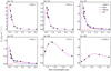 |
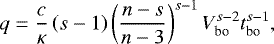
Fig. 6 Fit of a hot and a warm BB component to the evolution of the SED of SN 2015da. A warm component dominating at NIR wavelengths is clearly visible from t ≳ +430 d, increasing its strength with time. At t ≳ +730 d a single BB is sufficient to reproduce the SED at IR wavelengths (λ ≳ 1.2 μm). |
Main parameters of the BB fit to the observed SED evolution of SN 2015da.
Mass and temperature evolution of the dust shell for grains of different composition (graphite/silicates) and sizes.
3.1.2 Evolution of the pseudo-bolometric light curve
The evolution of the bolometric luminosity of SN 2015da was computed from the available photometric data in Tartaglia et al. (2016), integrating the observed SEDs without considering those regions not covered by the observations, hence only from the u to the W2 bands. The resulting “pseudo-bolometric” light curve shows a slow rise (≃ 100 d) with a bright peak luminosity ≃ 3.0 × 1043 erg s−1. However, the early SN bolometric light curves can be significantly underestimated without taking into account the UV contribution (see also the discussion in Tomasella et al. 2018). We therefore took the temperatures obtained fitting Eq. (3) to the observed SEDs to infer the scaling factor to account for the lack of observations at λ < 3500Å, assuming a blackbody form. Due to the strong contamination of Fe II lines at wavelengths bluer than ≃ 5000Å (see Sects. 3.2 and 3.1.1), at t > 400 d we fixed the temperature of the pseudo continuum to 5850 K, although we note that the correction at these epochs is small (less than 10%). We note, however, that this might still underestimate the UV contribution at early epochs, as shown by Dessart et al. (2015, their Fig. 13).
The resulting bolometric light curve, shown in Fig. 7, has a significantly shorter rise of ≃ 30 d, with a much brighter peak, ≃ 6.2 × 1043 erg s−1, more than a factor two brighter than our previous estimate, and more than three times higher than that inferred for SN 2010jl by Fransson et al. (2014). The UV contribution for SN 2010jl was, however, estimated from direct observations and the explosion is uncertain, hence its peak may have been missed, resulting in a possible brighter luminosity. In any case, this would make SN 2015da one of the brightest Type IIn SNe ever observed. The total radiated energy in the first 1233 d, after removing the IR contribution (likely due to a dust echo; see Sect. 3.1.1), is ≃ 1051 erg. This high value and the prominent narrow emission lines suggest that an ejecta-CSM interaction with a highly efficient conversion of kinetic energy into radiation is the main mechanism powering the light curve of SN 2015da (see, e.g., Fransson et al. 2014).
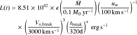
The luminosity evolution of SN 2015da can then be modeled in the context of an SN explosion within an extended and dense CSM (see Chevalier & Irwin 2011; Svirski et al. 2012; Ofek et al. 2014b). After CC, a radiation-mediated shock wave propagates outwards until it breaks through the stellar photosphere. If the progenitor is surrounded by a dense and extended CSM with an optical depth τCSM > c∕Vsh = τsh (where c is the speed of light and Vsh the velocity of the shock), the SN shock propagates into the CSM. As a consequence, the shock breakout signal is delayed, and the reverse-forward shock structure typical of interacting transients forms at the interface between the SN ejecta and the CSM (Chevalier & Fransson 1994). As the photon diffusion time drops below the shock expansion timescale (i.e., when τCSM ≃ τsh ≃ c∕Vs), the thermalized shock radiation escapes the CSM, releasing energy over timescales that may be much longer than those typically observed in windless breakouts (see Ofek et al. 2010; Chevalier & Irwin 2011). If the density of the CSM above the breakout layer is sufficiently high, the shock becomes collisionless, the photons are no longer trapped (Katz et al. 2012), and the kinetic energy of the ejecta is efficiently converted into radiation at a rate of 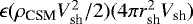 , where ɛ is the conversion efficiency, ρCSM the density of the CSM, and rsh and Vsh the radius and velocity of the shock, respectively (Svirski et al. 2012).
At later times, when the mass of the swept-up CSM is comparable to, or larger than, the ejected mass, the system can either enter a phase of energy (the Sedov–Taylor phase) or momentum conservation (“snowplow” phase; Svirski et al. 2012), which, in both cases, would result in a steeper decay of the observed luminosity. If the shock reaches the outer boundary of the dense CSM before this phase occurs, an even steeper drop in luminosity takes place.
Assuming spherical symmetry, Chevalier (1982b) showed that the density profiles of the SN ejecta and dense CSM can be described by power laws of the form 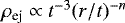 and ρCSM = qr−s, respectively. In a wind profile (s = 2), the density profile of the surrounding material canbe expressed by ρw = Ṁ∕(4πuwr2) (see, e.g., Chevalier & Fransson 2017), and therefore when we know the normalization constant q, it is possible to infer the mass-loss rate of the progenitor star during the last stages of its evolution12.
Assuming that the shock breakout occurs at τ ≈ c∕V, Ofek et al. (2014b) showed that the value of q can be estimated using
 (5)
(5)
where κ is the opacity (κ = 0.34 cm2 g−1 for electron scattering in a H-rich gas), c the speed of light, and Vbo is the shock velocity at the shock breakout Vs(tbo). Therefore, for s = 2, q is only a function of n and tbo. Using 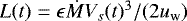 , Vs (tbo) can be expressed as a function of the energy conversion efficiency ɛ
![Mathematical equation: \begin{equation*} V_{\textrm{bo}}=t_{\textrm{bo}}^{(\alpha-1)/3}\left[2\pi\epsilon\frac{n-s}{n-3}\left(s-1\right)\frac{c}{\kappa L_0}\right]^{-1/3},\end{equation*}](/articles/aa/full_html/2020/03/aa36553-19/aa36553-19-eq10.png) (6)
(6)
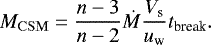
with L0 directly derived by fitting the bolometric light curve before the break with a power law. In a wind profile, q = Ṁ∕4πuw and the mass-loss rate of the progenitor star can be derived directly from the density profile of the CSM as a function of the wind expansion velocity uw, as Eq. (5) loses its dependence on Vbo. The mass of the CSM swept up by the shock at the time t can be expressed as a function of L0, tbo, n and s (see Eq. (21) in Ofek et al. 2014b), which, in a wind profile, can be expressed by:
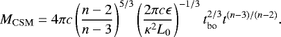 (7)
(7)
The pseudo-bolometric light curve of SN 2015da can be interpreted as the result of a SN shock propagating in a dense wind, with photon diffusion in the dense H-rich CSM being the dominant mechanism until t ≃ +150 d. This epoch corresponds to the onset of the broken power law describing the light curve, when the energy input from the shock directly corresponds to the observed luminosity. The “shock breakout” through the dense wind can then be estimated from the peak of the light curve at ≃ 30 d (see Fig. 7), while the observed break at t ≃ +290 d corresponds to the onset of the snowplow phase. On the other hand, as shown by Moriya (2014), this would result in a modest decay rate, and a more likely interpretation is the propagation of the shock into a CSM with a lower density, as also inferred from the narrow P-Cygni in the Hα profile (see Sect. 3.2.1).
At t ≥ +150 d, the bolometric light curve of SN 2015da is well-reproduced by a broken power law, with an early luminosity evolution described by L = 9.59 × 1049 t−0.92 erg s−1 followed by a much steeper decline with L ∝ t−3.98 erg s−1 until + 1233 d (subtracting the contribution of the IR luminosity at t ≥ +433 d; see Sect. 3.1.1), while the change in the power law index occurs around + 290 d.
Ofek et al. (2014b) showed that the value of n is related to the power law index α through the equation:
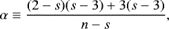 (8)
(8)
which, in a wind profile, gives n = 5.26 for α =−0.92. This value is considerably lower than that inferredfor SN 2010jl (n ≃ 7.6; Fransson et al. 2014). The relative time interval between the diffusion phase and break in the light curve is, however, considerably shorter for SN 2015da, which makes the determination of the power law index more uncertain.
Assuming that the time of the shock breakout coincides with the peak in luminosity in the diffusion dominated phase, tbo ≃ 30 d, and a wind velocity uw ≃ 100 km s−1 (see Sect. 3.2.1), Eq. (5) gives a mass-loss rate Ṁ = 0.66 M⊙ yr−1 for n =5.26. Equation (7) then gives a total mass of  M⊙ for the CSM swept up by the SN shock at t = tbreak = 290 d. Here, we scaled the efficiency to ɛ = 0.25 (Ofek et al. 2014a). Some support for a value of ɛ in this range comes from two-dimensional radiation hydrodynamics simulations of Type IIn SNe (Vlasis et al. 2016), who found an efficiency of ~30% for the conversion of kinetic energy to radiation. We emphasize, however, that this value is uncertain.
Alternatively, after the photon diffusion phase, the bolometric light curve can be expressed (for s = 2) as:
 (9)
(9)
(Fransson et al. 2014). Equation (9) gives the bolometric luminosity at tbreak as a function of the shock velocity at this epoch, Vbreak (or any other epoch). The mass of the swept up CSM can then be obtained from the same relation used to get Eq. (7):
 (10)
(10)
For low mass-loss rates, Vbo can be inferred from line profiles often observed from the shocked gas of interacting transients (see, e.g., the cases of SNe 1988Z, 2005ip and 2006jd; Turatto et al. 1993; Stritzinger et al. 2012, respectively). However, SN 2015da shows symmetric line profiles with broad wings typical of electron scattering from an outer un-shocked CSM at all epochs (see Sect. 3.2). Therefore, we could not estimate the velocity of the shock at the breakout directly from the spectra. Alternatively, the shock velocity at the time of the breakout can be derived using Eq. (6) for given values of ɛ, resulting in  km s−1 at t = tb0 = 30 d, and
  km s−1 at t = tbreak = 290 d.
Assuming a typical velocity Vs ≃ 3000 km s−1 at an age of one year, as inferred for other Type IIn SNe such as SNe 2010jl (Fransson et al. 2014) or 2013L (Taddia et al. in prep.), we can infer independent values for Ṁ and the mass of the swept up CSM, obtaining (adopting ɛ = 0.25)  , in agreement with our former estimate. The agreement between these two estimates gives some extra confidence in the choice of this parameter. The total CSM mass from Eq. (10) is therefore
  M⊙. Again, we point to the considerable uncertainty in this estimate from the assumed values of Vs and ɛ. In addition, we did not take into account possible variations in the kinetic energy conversion efficiency ɛ due to a high density gradient within the shocked regions (see, e.g., Tsuna et al. 2019).
It is of some interest to compare our simplified modeling with the detailed simulations by Dessart et al. (2015), using the Eulerian radiation-hydrodynamics code HERACLES (González et al. 2007). Although these were designed to model SN 2010jl and are one-dimensional simulations, they are of interest for understanding the effects of photon diffusion on the observed light curve through a qualitatively visual comparison.
Figure 8 shows that models X (Ṁ = 0.1 M⊙ yr−1) and Xm3 (Ṁ = 0.3 M⊙ yr−1) are able to roughly reproduce the early evolution of SN 2015da, with comparable rise times, although with lower luminosities. Model Xm6, with a higher mass-loss rate (0.6 M⊙ yr−1), gives roughly the correct luminosity, but with a slower rise time, while Xe3 (Ṁ = 0.1 M⊙ yr−1 and total energy of 3 × 1051 erg) seems to reproduce the rise time and the early (up to ≃150 d after explosion) part of the light curve after maximum well, although with a much higher peak luminosity. However, we note that the early light curve is uncertain due to the large bolometric correction from the assumed spectral shape in the UV. All these models correspond to a 9.8 M⊙ inner ejecta breaking through a dense CSM (with a total mass of 2.89 M⊙) with a wind density profile, uw = 100 km s−1, a constant temperature of 2000 K, and total kinetic energy of 1051 erg. While a more detailed modeling tuned to the observations of SN 2015da would be of obvious interest, a rough comparison between radiative transfer models and our estimates provides a comparable mass loss, although with a higher total CSM mass.
To account for these high values, we have to assume that a large fraction of the surrounding CSM was expelled by the progenitor star throughrepeated massive eruptive events like those occasionally experienced by LBV stars (see the case of the Great Eruption of η Car, e.g., Morris et al. 1999; Smith et al. 2003). On the other hand, the mass-loss rate and CSM mass inferred through Eqs. (5) and (7) are strongly dependent on the assumed value of tbo and s. Ofek et al. (2014a) showed that for s < 2, the shock is expected to break through near the edge of the CSM, and the model would not give a light curve with a power law decay lasting long enough to reproduce the light curve of SN 2010jl. We note, however, that SN 2015da shows a somewhat different behavior at t ≤ tbreak, with a significantly shorter first decline than that observed in SN 2010jl (see Fig. 7).
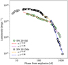 |
Fig. 7 Bolometric light curve of SN 2015da compared to that of SN 2010jl in logarithmic units. The best fit parameters for + 150 ≤ t ≤ +290 d and t >+290 d (+ 30 ≤ t ≤ +320 d and t >+320 d for SN 2010jl following Fransson et al. 2014 and Ofek et al. 2014b) are reported in the legend. |
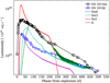 |
Fig. 8 Bolometric light curve of SN 2015da compared to models presented in Dessart et al. (2015) and bolometric light curve of SN 2010jl (computed as in Fransson et al. 2014). Model X has Ṁ = 0.1 M⊙ yr−1, model Xm3 Ṁ = 0.3 M⊙ yr−1, and model Xm6 Ṁ = 0.6 M⊙ yr−1. In all cases, the total energy is 1051 erg. Model Xe3 has Ṁ = 0.1 M⊙ yr−1 and total energy 3 × 1051 erg. |
3.2 Spectroscopy
The optical spectral evolution of SN 2015da is shown in Fig. 9, which includes a selection of spectra with the highest signal-to-noise ratios (S/Ns) and resolutions. The entire set of spectroscopic data is available, along with the photometric tables, through the Weizmann Interactive Supernova data REPository (WISEREP13; Yaron & Gal-Yam 2012). Our 2 NIR spectra are shown in Fig. 10, while a complete log of the spectroscopic observations is reported in Table A.6 and shown in Fig. A.1 in Appendix A.2.
At early phases, the spectra show classical features of Type IIn SNe, such as a blue continuum with prominent narrow H I (Hα to Hɛ); see Fig. 11 showing the early evolution of Hα and He I (λ5875 and λ7065) lines in emission. The strong Na I D doublet (λλ5890, 5896) is clearly visible until + 193 d, suggesting a highly extinguished local environment (see Sect. 2). At later phases, the spectral continuum fades and the He I λ5875 line dominates the spectral flux at these wavelengths. From the positions of the minima of the Na I D features observed in the DEIMOS spectrum we inferred a heliocentric recessional velocity of ≃ 2000 km s−1 that we adopt to set the observed spectra at rest wavelengths.
Early spectra (t≃ + 8 d) also show narrow circumstellar [N II] λ5755, broad O I λ8446 and narrow NIR H I features (Pa 8 to Pa 12), while Fe II lines (multiplets 42, 48 and 49) are visible, although faint, already at + 23 d, becoming more evident at later phases (t ≥ +110 d), where they start to contribute significantly to the shape of the blue pseudo-continuum (at λ ≲ 5800Å). At + 19 d we also identify Mg II λλ7877, 7896, λλ8214, 8235, and λλ9218, 9244. The NIR Ca II triplet starts to dominate the red part of the optical spectra from t ≃ +138 d, becoming most prominent at ≃505 d, when it starts to fade with respect to the spectral continuum.
The NIR H I lines become progressively stronger up to + 590 d whereafter they slowly decrease in strength. At + 35 d, the NIR spectrum is dominated by narrow H I (Paβ to Paζ) and He I (λ10830) lines.
Fitting a BB to the spectral continuum, we inferred the temperature evolution of the pseudo photosphere, slowly declining from ≃ 13 430 ± 355 K to ≃ 7180 ± 510 K during the first ≃240 d after explosion, in agreement with the one inferred from the SEDs (see Sect. 3.1.1). From t ≃ 193 d, the spectra show a blue excess at wavelengths shorter than ≃5500Å, becoming more evident at later epochs, observed throughout the remaining ~ 1300 d of the spectroscopic monitoring. The source of the excess is likely not thermal, since spectra at these wavelengths (λ < 5500−5800Å) are significantly affected by strong Fe II blends. On the other hand, late (t ≳100 d) blue excesses are common in interacting transients (see the cases of SNe 2006jc; Foley et al. 2007; Pastorello et al. 2007 and 2005ip; Smith et al. 2009b) and are likely due to the contribution of fluorescence from a number of blended Fe lines or to a “revitalized” late-time ejecta-CSM interaction with a low energy conversion efficiency (see, e.g., Smith et al. 2009b).
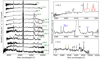 |
Fig. 9 Left:selection of optical spectra of SN 2015da with highest S/N, spectral coverage and resolution. Spectra were not corrected for extinction to facilitate the comparison at wavelengths bluer than ≃ 5000Å. Right: line identification on the + 23 d (first and second panel) and + 19 d (bottom panel) spectra. Phases refer to the estimated epoch of the explosion. |
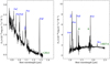 |
Fig. 10 NIR spectra of SN 2015da at + 26 d (left) and + 607 d (right). Phases refer to the estimated epoch of the explosion. |
3.2.1 The DEIMOS spectrum
A moderate-resolution spectrum (R ≃ 3600 from the [O I] sky lines) was obtained on 2015 February 23.66 UT (JD = 2 457 077.16, corresponding to t = +46 d; Program ID U063D, PI Filippenko), with the DEep Imaging Multi-Object Spectrograph (DEIMOS; Faber et al. 2003) mounted at the 10 m Keck II telescope at Mauna Kea. These data are available in the public section of the Keck Observatory Archive (KOA14).
The spectrum shows many marginally resolved Fe II lines with P-Cygni absorption features (multiplets 40, 42, 46, 48, 49, 74) or purely in emission (200, 40 apart from λ6516 and 49, with the possible exception of λ6113). We also identified a number of narrow lines purely in emission corresponding to other transitions, namely [N II] λ5755, He I λ5875 and Si II λλ6347, 6371 as well as a few other unidentified lines at 5568, 5587, 6318, 6332, and 6384/6385 Å. The Fe II λ5169 line, typically used to infer the photospheric expansion velocity in SNe, shows a faint narrow emission with a structured absorption component, a minimum of ≃ 10 km s−1, and a blue wing, possibly contaminated by a second component, extending up to ≃ 110 km s−1. Fe II lines are blueshifted15 by ≃ 40−50 km s−1, from whichwe infer minima of ≃ 50 km s−1 with a terminal velocity of 100−110 km s−1.
In Fig. 12, we zoom in on the DEIMOS spectrum in the region of Hα showing a narrow PCygni feature with a minimum blueshifted by ≃ 55 km s−1, and a terminal velocity of ≃ 110 km s−1 on top of a broader profile, typical of electron scattering, with wings showing a full-width-at-zero-intensity (FWZI) of ≃ 3 × 10³ km s−1.
To illustrate the dominance of electron scattering in the formation of the line profiles, we used the same Monte Carlo code as in Fransson et al. (2014). The input photons from recombination and collisions are emitted from the ionized region of the slowly moving “precursor shock” (Sutherland & Dopita 2017) and then undergo electron scattering in the same region, although most of them are emitted close to the shock. The main parameters of the fit are the optical depth to electron scattering, τe and the electron temperature, Te. Since the change in frequency in each scattering is  , to obtain a given FWHM, we need
  . The two parameters are therefore degenerate. In our calculations, we assumed Te = 104 K, and we did not attempt to model the resonance scattering by the Hα line giving rise to the narrow P Cygni profile.
In Fig. 12, we show the resulting fit, where the broad wings are well-reproduced by an exponential profile typical of electron scattering (Huang & Chevalier 2018). To obtain the observed FWHM at this epoch, we need  . This value is similar to the one obtained for SN 2010jl (Fransson et al. 2014), and it shows that the gas is optically thick to electron scattering. The narrow line in the model is due to un-scattered photons at zero velocity. These photons are scattered by the Hα line itself and form part of the P Cygni profile below ~ 200 km s−1. The fact that this results in a P Cygni profile means that the emission must come from a more extended region, producing both the absorption and emission component.
An immediate conclusion is that the emission from the inner parts of the ejecta (with respect to the forward shock), have an even higher optical depth. Emission lines from this region would therefore be washed out into a continuum, explaining why we do not observe broad lines from the expanding ejecta or post-shock gas.
3.2.2 Evolution of the H lines
Physical quantities inferred from the main Balmer lines (i.e., Hα and Hβ) and described in this section are reported in Table 5, as obtained through the IRAF task SPLOT, including FWHM velocities and equivalent widths (EWs). EWsfor Hα and Hβ show average values of ~880Å and ~ 75Å, respectively, in agreement with the distribution of values inferred for the sample of SNe IIn presented in Silverman et al. (2013), who also proposed weaker Hβ lines (with EW≃ 6Å, as well as the absence of He I λ5876 features) as a hallmark feature of Ia-CSM SNe. The values inferred for SN 2015da argue against a Type Ia-CSM interpretation for this object.
At t < +63 d, Balmer lines show narrow profiles purely in emission, with roughly constant FWHM velocities of ≃ 103 km s−1 and ≃ 1.7 × 10³ km s−1 for Hα and Hβ, respectively.All Balmer lines are well reproduced using a Lorentzian profile, and we do not see any trace of the narrow component observed in the higher resolution DEIMOS spectrum obtained at + 46 d (see Sect. 3.2.1). This is most likely due to an effect of resolution, as suggested by the appearance of the narrow component in the moderate-resolution spectra obtained at + 505 ≤ t ≤ +606 d, all having resolutions ≲10Å in the 6300−6800Å region.
From + 79 d, we note small deviations from a single Lorentzian profile in the blue wing of Hα (see Fig. 11) and a second Gaussian component is required to fit the entire profile. The Hβ line profile, on the other hand, is well-reproduced by a single Lorentzian component at all phases. A second component is required also at later phases, although at + 138 d Hα does not show significant asymmetries, and a single Lorentzian component is again sufficient to fit the entire profile (see Fig. 11). In the early NIR spectrum (+ 26 d), Paschen lines are marginally resolved (FWHM ≃ 600 km s−1) and show symmetric profiles centered at the corresponding rest wavelengths. At later phases (+ 607 d), we notice a broadening (FWHM ≃ 1100−1300 km s−1) in the Paγ and Pa β lines, with slightly blueshifted peaks of ≃ 100 km s−1 (≃40 km s−1 for Pa γ, which is strongly contaminated by the prominent He I λ10830 line), although the overall profiles are still well-reproduced by single symmetric Lorentzian (or Gaussian, for marginally resolved lines) profiles.
We note a similar evolution in Hα, with the centroid of the line progressively shifting toward bluer wavelengths with time, up to 300−500 km s−1 at t ≳ 833 d, where the uncertainty is due to the different S/N and resolutions of the spectra. This is highlighted in Fig. 11 (right panel), showing the evolution of Hα over selected phases. The Hα profile shows a broadening at t ≳ 100 d, which might be due to a gradual emergence of the emission from the shock, while the overall profile remains symmetric (see below).
In SN 2010jl, wavelength-dependent asymmetries and the apparent dimming of the red wings of emission components was used by Smith et al. (2012) and Gall et al. (2014) to suggest rapid dust formation in the SN ejecta as the possible cause of the IR excess. However, Fransson et al. (2014) showed that the profile of Hα remains symmetric with respect to a shifted centroid and attributed this shift to a bulk velocity of the emitting shell or to acceleration of the un-shocked CSM by the radiation field generated in the inner shocked regions. Following Fransson et al. (2014), we therefore mirrored the red wing of Hα with respect to the computed centroid of the line profile at each epoch. The resulting profiles are shown in Fig. 13 for a selection of spectra with high S/N and good resolution. As in SN 2010jl, no sign of asymmetries is seen at any epoch, suggesting that a macroscopic velocity is the most likely reason for the blueshift of the Hα profile of SN 2015da.
The evolution of the Hα and Hβ integrated luminosity is shown in Fig. 14. We note a rapid decline for both lines during the first 63 d, with the luminosity evolving from ≃ 6.58∕3.60 × 1041 erg s−1 to 5.46∕2.94 × 1041 erg s−1 for Hα/Hβ, respectively. The luminosity shows a subsequent re-brightening up to 1.39∕0.29 × 1042 erg s−1 during the following ≃180 d, with an offset of ≃+30 d with respect to the onset of the re-brightening observed in SN 2010jl (assuming JD = 2 455 479 as the explosion epoch for SN 2010jl; Fransson et al. 2014). The integrated luminosities show a further decline at later phases, until + 706 d, when it sets at 1.94∕0.33 × 1041, staying roughly constant for the remaining ≃750 d. In SN 2015da, the Hα/Hβ ratio increases monotonically up to ≃+560 d, when it settles at a roughly constant value of ≃5.7, while at + 1458 d, it drops again to 2.92, showing a quite different evolution with respect to that of SN 2010jl. This different behavior might be attributed to the blue pseudo continuum contamination of the spectra at t ≳ 228 d, which can bias the integrated luminosity inferred for Hβ (see Sect. 3.2 and Fig. 14, upper panel).
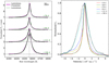 |
Fig. 11 Left: fit to the Hα line profiles on the + 79 d, + 94 d, + 111 d and + 138 d spectra using a combination of Lorentzian and Gaussian functions. Right: evolution of the continuum-subtracted Hα profile over a selection of phases. The line profiles were normalized to their peak values in order to highlight their evolution. Phases referto the estimated epoch of the explosion. |
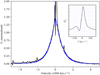 |
Fig. 12 Hα line profile observed in the + 46 d Keck DEIMOS spectrum of SN 2015da along with a fit to the line profile from electron scattering. The line profile below ± 200 km s−1, in the model from un-scattered photons, is affected by the resonance line scattering in the Hα transition and was notmodeled. |
Main parameters of the BB fit to the observed SED evolution of SN 2015da.
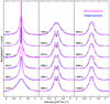 |
Fig. 13 Hα profiles at selected epochs, redshifted to the line rest wavelength (blue) and mirrored with respect to the computed centroids (magenta). Lines show highly symmetric profiles, with blue and red wings overlapping almost perfectly at all phases. Small asymmetries in the top part of the lines are due to the presence of the narrow P Cygni features, more evident in the higher resolution spectra. Phases refer to the estimated epoch of the explosion. |
3.3 The progenitor star
The field ofSN 2015da was monitored by the Palomar Transient Factory (PTF16), which imaged its host galaxy with a roughly constant cadence from 2009 March 17 to 2014 May 28 (see Table A.2). Frames were recovered through the NASA/IPAC Infrared Science Archive17. We could not detect traces of pre-SN variability down to g ≃−16.1 mag or − 15 mag, assuming a distance of 53.2 Mpc and the total extinction reported in Sect. 2. LBVs are among the most luminous stars known, and typically have absolute magnitudes MR ≃−9 mag in quiescence. On the other hand, they occasionally experience nonterminal major eruptive events, like the ones observed in η−Car in the 19th century (e.g., Smith & Frew 2011), producing optical transients that mimic the behavior of SNe IIn (hence dubbed “SN impostors”; Van Dyk et al. 2000; Maund et al. 2006), although with fainter absolute magnitudes (Mpeak ≃−14 mag, e.g., Tartaglia et al. 2015, 2016). In addition, we cannot rule out a larger value of reddening in the environment of the progenitor star before explosion. An SN explosion in a dusty environment is expected to produce a dust-free cavity within a radius directly dependent on the peak luminosity of the transient. Dwek (1983) showed that an SN with Lpeak = 1010 L⊙ can produce a cavity of 5.1 × 1017 cm, depending on the chemical composition, size of the dust gains, density and optical depth of the shell. Therefore, a larger amount of dust could survive less luminous outbursts. It is therefore possible that the local extinction in the environment of SN 2015da was higher during the pre-SN stages than was estimated in Sect. 2, possibly masking multiple LBV–like outbursts. In this scenario, the available observations would not put sensible constraints on the pre-explosion variability of the precursor.
The prominent narrow [N II] line visible in the spectra almost at all phases is indicative of a possible nitrogen enrichment of the narrow-line region of the CSM, which in turn might indicate a large enrichment of CNO processed gas. Significant CNO enrichments have been observed in SN ejecta or CSM for a small number of CC SNe (see, e.g., Fransson et al. 2005, and references therein), as well as evolved massive stars such as LBVs. Unfortunately, most of the diagnostic lines commonly used for CNO analyses are out of the observed spectral range (e.g., C III, C IV, N III], N IV], and O III], all at λ < 2000Å; Fransson et al. 2014), and we therefore did not have the sufficient spectroscopic coverage or resolution to perform a detailed analysis.
On the other hand, from the narrow Hα P Cygni absorption observed in the higher resolution DEIMOS spectrum at + 46 d, we inferred a wind velocity of ≃ 100 km s−1 (similar to that of SN 2010jl), suggesting a very massive star as a viable progenitor for SN 2015da. This corresponds to the lower end of the range of typical velocities inferred for LBVs (102 −103; e.g. Smith et al. 2011), which, on the other hand, is significantly higher than those displayed by red supergiants (RSG, 10− 50 km s−1; e.g. Jura & Kleinmann 1990). In addition, the total mass of the CSM inferred from our analysis of the pseudo-bolometric light curve (≳ 5.5M⊙; see Sect. 3.1.2) is more than a factor of five higher than that expected to be lost by a lower mass star during the RSG phase (< 1M⊙ for a star with an initial mass of 16 M⊙; Beasor & Davies 2018). As a consequence, there are a number of consistent, although not compelling, indications suggesting that the progenitor of SN 2015da was an LBV star.
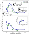 |
Fig. 14 Evolution of the integrated luminosity of the most prominent Balmer lines (Hα and Hβ) compared to those inferred for SN 2010jl. Insets in the upper panel show representative spectra during the different phases of the evolution of SN 2015da. The inset in the bottom panel shows the evolution of the Hα/Hβ ratio compared to that computed for SN 2010jl. |
4 Summary and conclusions
In this paper, we reported the main results of the photometric and spectroscopic follow-up of the Type IIn SN 2015da, exploded in the relatively nearby (D ≃ 53.2 Mpc) host galaxy NGC 5337.
SN 2015da is a long-lasting Type IIn SN discovered soon after explosion and with well-sampled photometric and spectroscopic follow-up from the optical to MIR wavelengths. This makes it one of the best followed SN IIn, with, to date, more than four years of collected data. Follow-up campaigns of this nearby optical transient are still ongoing both in the optical and NIR and MIR domains, and additional data could help us to better constrain the physical properties of the explosion, its dusty environment, and ultimately the nature of its progenitor star.
The transient exploded in a highly obscured environment, contributing a reddening of E(B−V) = 0.97 mag (AV ≃ 3 mag assuming a canonical extinction law with RV = 3.1) in the direction of SN 2015da. The IR excess observed from + 433 d suggests that the IR luminosity is most likely produced by radiatively heated dust. This conclusion is supported by the shape of the Hα line profiles, which show symmetric wings with respect to their centroids at all phases, while alternative explanations, like rapid formation oflarge dust grains at the interface between the forward and reverse shock, would result in strong asymmetries in the line shape. On the other hand, given the simplicity of the models adopted here and the assumptions made, we cannot definitely rule out anyof the possible emission mechanisms.
The analysis of the pseudo-bolometric light curve of SN 2015da revealed an extended CSM with a total mass 5.5−10.3M⊙ (assuming an energy conversion efficiency ɛ = 0.25), while wind velocities suggest a very massive precursor, possibly an LBV, as a viable progenitor for SN 2015da. This conclusion is supported by the very high mass-loss rate inferred from the evolution of the pseudo-bolometric luminosity (Ṁ ≃ 0.6−0.7 M⊙ yr−1), which indicates that multiple outbursts during a long-lasting eruptive phase, similar to those observed in other SN impostors such as SN 2000ch (Wagner et al. 2004; Pastorello et al. 2010) are responsible for the dense CSM surrounding the progenitor star at the time of its explosion. We note, however, that the upper CSM mass limit would require a progenitor that retained a massive envelope until the very last phases of its evolution. According to the Geneva stellar evolutionary models (Hirschi et al. 2004), this is problematic at solar metallicity. For example, a nonrotating 25 M⊙ star has an envelope mass of ≃ 10M⊙ at the point of explosion, while a more massive (or rotating) star would lose even more mass to then explode as a stripped-envelope SN. While this envelope mass is larger than the ejected CSM, it would require that the “entire” envelope was ejected just before explosion. If we assume that only some fraction of the envelope can be ejected immediately prior to CC, we must turn to lower metallicity models, which, on the other hand, have commensurately smaller Ṁ. On the other hand, even at SMC metallicity, it is hard to form a H-rich star that has an envelope mass exceeding 10 M⊙ at the time of CC. At even lower metallicity, for example, Z = 10−5, wind-driven mass loss is much smaller, and it is possible to form a progenitor with a ZAMS mass of 60 M⊙ that will explode as a Type II SN (Meynet & Maeder 2002). However, while this was plausible for SN 2010jl that exploded in a faint irregular galaxy, NGC 5337 is a normal spiral, with a roughly solar metallicity (see Sect. 2). One possibility is that SN 2015da is hosted in a faint dwarf satellite of NGC 5337, which is by chance projected on the sky towards towards the main galaxy. Future spectroscopy at the site of SN 2015da after the SN has faded may allow us to measure the local metallicity, or, alternatively, to identify a kinematically distinct dwarf host. Without this information, the contradiction between the nearly solar metallicity host and the requirement for a low metallicity progenitor remains a puzzle.
Acknowledgements
We thank Marco Berton, Sina Chen, Fabio Briganti, Fabio Martinelli, Emmanuel Conseil, Stan Howerton, Masanori Mizutani and Kunihiro Shima for their help with the observations of SN 2015da. We are also grateful to our late friend Alex Dimai, whose observations have been used in this study. We gratefully acknowledge support from the Knut and Alice WallenbergFoundation. The Oskar Klein Centre is funded by the Swedish Research Council. We acknowledge the support of the staff of the Xinglong 2.16 m telescope. This work was partially supported by the Open Project Program of the Key Laboratory of Optical Astronomy, National Astronomical Observatories, Chinese Academy of Sciences. M.F. is supported by a Royal Society – Science Foundation Ireland University Research Fellowship. J.H. acknowledges financial support from the Finnish Cultural Foundation and the Vilho, Yrjö and Kalle Väisälä Foundation of the Finnish Academy of Science and Letters. Research by D.J.S. is supported by NSF grants AST-1821987, AST-1821967, AST-1813708, AST-1813466 and AST-1908972. S.B., L.T.and M.T. are partially supported by the PRIN-INAF 2016 with the project “Towards the SKA and CTA era: discovery, localisation, and physics of transient sources” (PI: M. Giroletti). N E.-R. acknowledges support from the Spanish MICINN grant ESP2017–82674–R and FEDER funds. D.A.H., C.M., and G.H. were supported by NSF AST-1313484 The work of X.W. is supported by the National Natural Science Foundation of China (NSFC grants 11325313, 11633002, and 11761141001), and the National Program on Key Research and Development Project (grant no. 2016YFA0400803). Research by S.V. is supported by NSF grant AST-1813176. J.Z. is supported by the National Natural Science Foundation of China (NSFC, grants 11773067, 11403096), the Youth Innovation Promotion Association of the CAS (grants 2018081), and the Western Light Youth Project. Based on observations collected at: ESO La Silla Observatory under program “Optical & NIR monitoring of bright supernovae with REM” during AOT30. The Gemini Observatory, under program GN–2016B-Q-57, which is operated by the Association of Universities for Research in Astronomy, Inc., under a cooperative agreement with the NSF on behalf of the Gemini partnership: the National Science Foundation (United States), the National Research Council (Canada), CONICYT (Chile), Ministerio de Ciencia, Tecnología e Innovación Productiva (Argentina), and Ministério da Ciência, Tecnologia e Inovação (Brazil). Tthe Nordic Optical Telescope, operated by the Nordic Optical Telescope Scientific Association and the Gran Telescopio Canarias (GTC), both installed at the Spanish Observatorio del Roque de los Muchachos of the Instituto de Astrofìsica de Canarias, on the island of La Palma (Spain). The Copernico Telescope (Asiago, Italy) operated by INAF – Osservatorio Astronomico di Padova. The 3 m Shane Reflector, located at the Lick Observatory (7281 Mt Hamilton Rd, Mt Hamilton, CA 95140, USA.) owned and operated by the University of California. This work makes use of observations from the Las Cumbres Observatory network of telescopes. We acknowledge the support of the staff of the Li–Jiang 2.4 m telescope (LJT). Funding for the LJT has been provided by the Chinese Academy of Sciences (CAS) and the People’s Government of Yunnan Province. The LJT is jointly operated and administrated by Yunnan Observatories and Center for Astronomical Mega–Science, CAS. This research has made use of the Keck Observatory Archive (KOA), which is operated by the W. M. Keck Observatoryand the NASA Exoplanet Science Institute (NExScI), under contract with the National Aeronautics and Space Administration. Some of the data presented herein were obtained at the W. M. Keck Observatory, which is operated as a scientific partnership among the California Institute of Technology, the University of California and the National Aeronautics and Space Administration. The Observatory was made possible by the generous financial support of the W. M. Keck Foundation. The authors wish to recognize and acknowledge the very significant cultural role and reverence that the summit of Mauna Kea has always had within the indigenous Hawaiian community. We are most fortunate to have the opportunity to conduct observations from this mountain. This publication makes use of data products from NEOWISE, which is a project of the Jet Propulsion Laboratory/California Institute of Technology, founded by the Planetary Science Division of the National Aeronautics and Space Administration. This research has made use of the Keck Observatory Archive (KOA), which is operated by the W. M. Keck Observatory and the NASA Exoplanet Science Institute (NExScI), under contract with the National Aeronautics and Space Administration. This research has made use of the NASA/IPAC Extragalactic Database (NED) which is operated by the Jet Propulsion Laboratory, California Institute of Technology, under contract with the National Aeronautics and Space Administration. This research has made use of the NASA/IPAC Infrared Science Archive, which is operated by the Jet Propulsion Laboratory, California Institute of Technology, under contract with the National Aeronautics and Space Administration. This publication makes use of data products from the Two Micron All Sky Survey, which is a joint project of the University of Massachusetts and the Infrared Processing and Analysis Center/California Institute of Technology, funded by the National Aeronautics and Space Administration and the National Science Foundation. Funding for the Sloan Digital Sky Survey (SDSS) has been provided by the Alfred P. Sloan Foundation, the Participating Institutions, the National Aeronautics and Space Administration, the National Science Foundation, the U.S. Department of Energy, the Japanese Monbukagakusho, and the Max Planck Society. The SDSS Web site is http://www.sdss.org/. This publication makes use of data products from the Wide-field Infrared Survey Explorer, which is a joint project of the University of California, Los Angeles, and the Jet Propulsion Laboratory/California Institute of Technology, funded by the National Aeronautics and Space Administration. The SDSS is managed by the Astrophysical Research Consortium (ARC) for the Participating Institutions. The Participating Institutions are The University of Chicago, Fermilab, the Institute for Advanced Study, the Japan Participation Group, The Johns Hopkins University, Los Alamos National Laboratory, the Max-Planck-Institute for Astronomy (MPIA), the Max-Planck-Institute for Astrophysics (MPA), New Mexico State University, University of Pittsburgh, Princeton University, the United States Naval Observatory, and the University of Washington. The intermediate Palomar Transient Factory project is a scientific collaboration among the California Institute of Technology, Los Alamos National Laboratory, the University of Wisconsin, Milwaukee, the Oskar Klein Center, the Weizmann Institute of Science, the TANGO Program of the University System of Taiwan, and the Kavli Institute for the Physics and Mathematics of the Universe. IRAF is distributed by the National Optical Astronomy Observatory, which is operated by the Association of Universities for Research in Astronomy (AURA) under a cooperative agreement with the National Science Foundation. SNOOPY is a package for SN photometry using PSF fitting and/or template subtraction developed by E. Cappellaro. A package description can be found at http://sngroup.oapd.inaf.it/snoopy.html. FOSCGUI is a graphic user interface aimed at extracting SN spectroscopy and photometry obtained with FOSC-like instruments. It was developed by E. Cappellaro. A package description can be found at http://sngroup.oapd.inaf.it/foscgui.html.
Appendix A Observations and data reduction
The follow-up campaign of SN 2015da spanned a period of more than 1500 d after the SNexplosion and involved a number of collaborations and facilities. The names of the telescopes and instruments used are reportedin Tables A.1–A.4 (available at the CDS), and A.6.
A.1 Photometric data
Optical photometric data were mainly obtained using the telescopes of the Las Cumbres Observatory18 network (Brown et al. 2013) within the Supernova Key Project, while most of the NIR data and additional optical photometry were provided by the NUTS collaboration19, using the 2.56 m Nordic Optical Telescope (NOT, at the Observatorio del Roque de los Muchacos, La Palma, Spain) with NOTCam and ALFOSC. Optical data were also collected using the 1.82 m Copernico Telescope (at the INAF Osservatorio Astronomico di Asiago, Italy) with AFOSC and iPTF, the automated Mount Palomar 60 inch (P60) and the 48 inch Samuel Oschin (P48) telescopes. The iPTF survey did not monitor this part of the sky at all in 2015, so the transient was only detected by iPTF in March 2016, which is the reason why it was internally dubbed iPTF16tu. iPTF then followed the object for a full year until the end of the survey. Early data covering the rise to maximum light and a few additional epochs were provided by amateurs and calibrated to the R band. These data helped constrain the explosion epoch and the rise of SN 2015da (see Sect. 3.1).
NIR photometry was almost entirely provided by NUTS using the NOT with NOTCam, while early data around maximum were provided by the ESO 0.6 m Rapid Eye Mount telescope in La Silla (Chile). One additional NIR epoch was obtained using the Near Infrared Camera Spectrometer (NICS20) mounted at the 3.58 m Telescopio Nazionale Galileo (TNG) located at the Observatorio del Roque de los Muchachos in La Palma (Spain).
Optical and NIR pre-reduction steps were performed using standard IRAF tasks. NOTCam frames pre-reduced using an adapted version of the external IRAF package NOTCAM21, using bad pixel masking, differential flat-fielding method, sky subtraction, distortion correction, and stacking of dithered images. Final magnitudes were mostly obtained using the SuperNOva PhotometrY (SNOOPY22) pipeline and calibrated on a local sequence of stars obtained through the Sloan Digital Sky Survey (SDSS23) (for the optical frames) and the Two Micron All Sky Survey (2MASS24) catalogs. UBV RI magnitudes of the reference stars were obtained transforming the SDSS magnitudes following Chonis & Gaskell (2008). Magnitudes of the local standard stars are provided in Table A.5. P60 data were reduced using the dedicated pipeline described in Fremling et al. (2016).
MIR magnitudes were obtained as detailed below. For every pass, after a quick check to verify that the SN did not show rapid variations, all high-quality images (obtained typically within 3− 5 d) available in the NEOWISE 2019 Data Release have been co-added25 and retrieved. The SN exploded in a region in which the galaxy background was still significant, while the spatial resolution was relatively poor (≥6 arcsec). We therefore decided to apply the galaxy background subtraction method. To this aim, we use the averages of all images acquired during the year 2014, meaning before explosion, as background in both bands. After accurate re-entering, the images were ready to be subtracted, satisfactorily removing the galaxy, and leaving the SN alone. On the subtraction image we performed aperture photometry with aperture of eight and nine pixels. We then applied the aperture correction determined by applying the same aperture on a number of nearby, isolated reference stars of the same magnitude of the SN, present in the AllWISE Source Catalog. Following these prescriptions, the W1 and W2 magnitudes of SN 2015da reported in Table A.4 are on the same scale as the AllWISE catalog.
A.2 Spectroscopic data
The spectroscopic follow-up campaign was carried out mostly using the NOT with ALFOSC and the 1.82 m Copernico Telescope with AFOSC, and the data were reduced using the dedicated pipeline FOSCGUI26. Three additional spectra were obtained using the 2 m Faulkes Telescope North (FTN) telescope with FLOYDS of the Las Cumbres Observatory network. Spectra at different phases were provided by the TNG with DOLORes, the 10.4 m Gran Telescopio Canarias (GTC, located at the Observatorio del Roque de los Muchachos in La Palma) with OSIRIS, the 3 m Donald Shane Telescope (at the Lick Observatory in San Jose, California, USA) with KAST and the 200 inch Hale telescope with DBSP at the Mount Palomar Observatory (San Diego, California, USA). All these spectra were reduced using standard IRAF tasks. The classification spectrum was obtained using the Lijiang 2.4 m telescope (LJT) at the Lijiang Observatory of Yunnan Observatories with YFOSC, which also provided three early-phase spectra (+ 11, + 19 and + 26 d after explosion). Two additional early-phase spectra (+10 and +36 d) were obtained using the ZTA 2.6 m telescope located at the Byurakan Astrophysical Observatory (BAO, Armenia) with XLT. All these spectra were reduced using standard IRAF tasks. NIR spectra were provided by the TNG using NICS and reduced using IRAF tasks, and the 8.1 m Gemini North telescope (located at the Mauna Kea Observatory, Hawaii, USA) using the Gemini Near-InfraRed Spectrograph (GNIRS), reduced as in Hsiao et al. (2019). A complete set of optical spectra is shown in Fig. A.1.
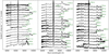 |
Fig. A.1 Complete set of optical spectroscopic observations of SN 2015da. Spectra were not corrected for extinction to facilitate the comparison at wavelengths bluer than ≃ 5000Å. Phases referto the estimated epoch of the explosion. |
Local sequence of stars used for the optical and NIR photometric calibration.
Log of the optical spectroscopic observations of SN 2015da.
References
- Adelman-McCarthy, J. K., Agüeros, M. A., Allam, S. S., et al. 2006, ApJS, 162, 38 [NASA ADS] [CrossRef] [Google Scholar]
- Agnoletto, I., Benetti, S., Cappellaro, E., et al. 2009, ApJ, 691, 1348 [NASA ADS] [CrossRef] [Google Scholar]
- Aldering, G., Antilogus, P., Bailey, S., et al. 2006, ApJ, 650, 510 [NASA ADS] [CrossRef] [Google Scholar]
- Alloin, D., Collin-Souffrin, S., Joly, M., & Vigroux, L. 1979, A&A, 78, 200 [Google Scholar]
- Andrews, J. E., Clayton, G. C., Wesson, R., et al. 2011, AJ, 142, 45 [NASA ADS] [CrossRef] [Google Scholar]
- Asplund, M., Grevesse, N., Sauval, A. J., & Scott, P. 2009, ARA&A, 47, 481 [NASA ADS] [CrossRef] [Google Scholar]
- Balberg, S., & Loeb, A. 2011, MNRAS, 414, 1715 [NASA ADS] [CrossRef] [Google Scholar]
- Beasor, E. R., & Davies, B. 2018, MNRAS, 475, 55 [NASA ADS] [CrossRef] [Google Scholar]
- Benetti, S., Cappellaro, E., Turatto, M., et al. 2006, ApJ, 653, L129 [NASA ADS] [CrossRef] [MathSciNet] [Google Scholar]
- Bohlin, R. C., Savage, B. D., & Drake, J. F. 1978, ApJ, 224, 132 [NASA ADS] [CrossRef] [Google Scholar]
- Borish, H. J., Huang, C., Chevalier, R. A., et al. 2015, ApJ, 801, 7 [NASA ADS] [CrossRef] [Google Scholar]
- Botticella, M. T., Smartt, S. J., Kennicutt, R. C., et al. 2012, A&A, 537, A132 [NASA ADS] [CrossRef] [EDP Sciences] [Google Scholar]
- Bottinelli, L., Gouguenheim, L., Paturel, G., & Teerikorpi, P. 1995, A&A, 296, 64 [NASA ADS] [Google Scholar]
- Brown, T. M., Baliber, N., Bianco, F. B., et al. 2013, PASP, 125, 1031 [NASA ADS] [CrossRef] [Google Scholar]
- Cardelli, J. A., Clayton, G. C., & Mathis, J. S. 1989, ApJ, 345, 245 [NASA ADS] [CrossRef] [Google Scholar]
- Chevalier, R. A. 1982a, ApJ, 258, 790 [NASA ADS] [CrossRef] [Google Scholar]
- Chevalier, R. A. 1982b, ApJ, 259, 302 [NASA ADS] [CrossRef] [Google Scholar]
- Chevalier, R. A., & Fransson, C. 1994, ApJ, 420, 268 [NASA ADS] [CrossRef] [Google Scholar]
- Chevalier, R. A., & Fransson, C. 2017, Thermal and Non-thermal Emission from Circumstellar Interaction (Berlin: Springer), 875 [Google Scholar]
- Chevalier, R. A., & Irwin, C. M. 2011, ApJ, 729, L6 [Google Scholar]
- Chonis, T. S., & Gaskell, C. M. 2008, AJ, 135, 264 [NASA ADS] [CrossRef] [Google Scholar]
- Chugai, N. N. 2001, MNRAS, 326, 1448 [NASA ADS] [CrossRef] [Google Scholar]
- Deng, J., Kawabata, K. S., Ohyama, Y., et al. 2004, ApJ, 605, L37 [NASA ADS] [CrossRef] [Google Scholar]
- Denicoló, G., Terlevich, R., & Terlevich, E. 2002, MNRAS, 330, 69 [NASA ADS] [CrossRef] [Google Scholar]
- Dessart, L., Audit, E., & Hillier, D. J. 2015, MNRAS, 449, 4304 [NASA ADS] [CrossRef] [Google Scholar]
- Di Carlo, E., Massi, F., Valentini, G., et al. 2002, ApJ, 573, 144 [NASA ADS] [CrossRef] [Google Scholar]
- Dilday, B., Howell, D. A., Cenko, S. B., et al. 2012, Science, 337, 942 [NASA ADS] [CrossRef] [Google Scholar]
- Draine, B. T., & Lee, H. M. 1984, ApJ, 285, 89 [Google Scholar]
- Dwek, E. 1983, ApJ, 274, 175 [NASA ADS] [CrossRef] [Google Scholar]
- Dwek, E. 1985, ApJ, 297, 719 [NASA ADS] [CrossRef] [Google Scholar]
- Elias-Rosa, N., Benetti, S., Cappellaro, E., et al. 2006, MNRAS, 369, 1880 [NASA ADS] [CrossRef] [Google Scholar]
- Faber, S. M., Phillips, A. C., Kibrick, R. I., et al. 2003, Proc. SPIE, 4841, 1657 [NASA ADS] [CrossRef] [Google Scholar]
- Ferlet, R., Vidal-Madjar, A., & Gry, C. 1985, ApJ, 298, 838 [NASA ADS] [CrossRef] [Google Scholar]
- Foley, R. J., Smith, N., Ganeshalingam, M., et al. 2007, ApJ, 657, L105 [NASA ADS] [CrossRef] [Google Scholar]
- Fox, O., Skrutskie, M. F., Chevalier, R. A., et al. 2009, ApJ, 691, 650 [NASA ADS] [CrossRef] [Google Scholar]
- Fox, O. D., Chevalier, R. A., Dwek, E., et al. 2010, ApJ, 725, 1768 [NASA ADS] [CrossRef] [Google Scholar]
- Fox, O. D., Chevalier, R. A., Skrutskie, M. F., et al. 2011, ApJ, 741, 7 [NASA ADS] [CrossRef] [Google Scholar]
- Fox, O. D., Filippenko, A. V., Skrutskie, M. F., et al. 2013, AJ, 146, 2 [NASA ADS] [CrossRef] [Google Scholar]
- Fox, O. D., Silverman, J. M., Filippenko, A. V., et al. 2015a, MNRAS, 447, 772 [NASA ADS] [CrossRef] [Google Scholar]
- Fox, O. D., Smith, N., Ammons, S. M., et al. 2015b, MNRAS, 454, 4366 [NASA ADS] [CrossRef] [Google Scholar]
- Fransson, C. 1984, A&A, 133, 264 [NASA ADS] [Google Scholar]
- Fransson, C., Chevalier, R. A., Filippenko, A. V., et al. 2002, ApJ, 572, 350 [NASA ADS] [CrossRef] [Google Scholar]
- Fransson, C., Challis, P. M., Chevalier, R. A., et al. 2005, ApJ, 622, 991 [NASA ADS] [CrossRef] [Google Scholar]
- Fransson, C., Ergon, M., Challis, P. J., et al. 2014, ApJ, 797, 118 [NASA ADS] [CrossRef] [Google Scholar]
- Fremling, C., Sollerman, J., Taddia, F., et al. 2016, A&A, 593, A68 [NASA ADS] [CrossRef] [EDP Sciences] [Google Scholar]
- Gal-Yam, A. 2019, ARA&A, 57, 305 [NASA ADS] [CrossRef] [Google Scholar]
- Gal-Yam, A., & Leonard, D. C. 2009, Nature, 458, 865 [NASA ADS] [CrossRef] [PubMed] [Google Scholar]
- Gall, C., Hjorth, J., Watson, D., et al. 2014, Nature, 511, 326 [NASA ADS] [CrossRef] [Google Scholar]
- Garavini, G., Folatelli, G., Goobar, A., et al. 2004, AJ, 128, 387 [NASA ADS] [CrossRef] [Google Scholar]
- Gerardy, C. L., Fesen, R. A., Nomoto, K., et al. 2002, ApJ, 575, 1007 [NASA ADS] [CrossRef] [Google Scholar]
- González, M., Audit, E., & Huynh, P. 2007, A&A, 464, 429 [NASA ADS] [CrossRef] [EDP Sciences] [Google Scholar]
- Graham, J. R., & Meikle, W. P. S. 1986, MNRAS, 221, 789 [NASA ADS] [CrossRef] [Google Scholar]
- Hakobyan, A. A., Mamon, G. A., Petrosian, A. R., Kunth, D., & Turatto, M. 2009, A&A, 508, 1259 [NASA ADS] [CrossRef] [EDP Sciences] [Google Scholar]
- Hamuy, M., Phillips, M. M., Suntzeff, N. B., et al. 2003, Nature, 424, 651 [NASA ADS] [CrossRef] [Google Scholar]
- Herbig, G. H. 1995, ARA&A, 33, 19 [NASA ADS] [CrossRef] [Google Scholar]
- Hirschi, R., Meynet, G., & Maeder, A. 2004, A&A, 425, 649 [NASA ADS] [CrossRef] [EDP Sciences] [Google Scholar]
- Hsiao, E. Y., Phillips, M. M., Marion, G. H., et al. 2019, PASP, 131, 014002 [NASA ADS] [CrossRef] [Google Scholar]
- Huang, C., & Chevalier, R. A. 2018, MNRAS, 475, 1261 [NASA ADS] [CrossRef] [Google Scholar]
- Inserra, C., Fraser, M., Smartt, S. J., et al. 2016, MNRAS, 459, 2721 [NASA ADS] [CrossRef] [Google Scholar]
- Jura, M., & Kleinmann, S. G. 1990, ApJS, 73, 769 [NASA ADS] [CrossRef] [Google Scholar]
- Kankare, E., Ergon, M., Bufano, F., et al. 2012, MNRAS, 424, 855 [NASA ADS] [CrossRef] [Google Scholar]
- Katz, B., Sapir, N., & Waxman, E. 2012, ApJ, 747, 147 [NASA ADS] [CrossRef] [Google Scholar]
- Kiewe, M., Gal-Yam, A., Arcavi, I., et al. 2012, ApJ, 744, 10 [NASA ADS] [CrossRef] [Google Scholar]
- Kotak, R., Meikle, W. P. S., Adamson, A., et al. 2004, MNRAS, 354, L13 [NASA ADS] [CrossRef] [EDP Sciences] [Google Scholar]
- Laor, A., & Draine, B. T. 1993, ApJ, 402, 441 [NASA ADS] [CrossRef] [Google Scholar]
- Li, W., Leaman, J., Chornock, R., et al. 2011, VizieR Online Data Catalog: VII/41 [Google Scholar]
- López-Sánchez, Á. R., Dopita, M. A., Kewley, L. J., et al. 2012, MNRAS, 426, 2630 [NASA ADS] [CrossRef] [Google Scholar]
- Mattila, S., Meikle, W. P. S., Lundqvist, P., et al. 2008, MNRAS, 389, 141 [NASA ADS] [CrossRef] [Google Scholar]
- Mauerhan, J. C., Smith, N., Silverman, J. M., et al. 2013, MNRAS, 431, 2599 [NASA ADS] [CrossRef] [Google Scholar]
- Maund, J. R., Smartt, S. J., Kudritzki, R. P., et al. 2006, MNRAS, 369, 390 [NASA ADS] [CrossRef] [Google Scholar]
- Mauron, N., & Josselin, E. 2011, A&A, 526, A156 [NASA ADS] [CrossRef] [EDP Sciences] [Google Scholar]
- Meynet, G., & Maeder, A. 2002, A&A, 390, 561 [NASA ADS] [CrossRef] [EDP Sciences] [Google Scholar]
- Moriya, T. J. 2014, A&A, 564, A83 [NASA ADS] [CrossRef] [EDP Sciences] [Google Scholar]
- Morris, P. W., Waters, L. B. F. M., Barlow, M. J., et al. 1999, Nature, 402, 502 [NASA ADS] [CrossRef] [Google Scholar]
- Nyholm, A., Sollerman, J., Tartaglia, L., et al. 2020, A&A, accepted https://doi.org/10.1051/0004-6361/201836097 [Google Scholar]
- Ofek, E. O., Cameron, P. B., Kasliwal, M. M., et al. 2007, ApJ, 659, L13 [CrossRef] [Google Scholar]
- Ofek, E. O., Rabinak, I., Neill, J. D., et al. 2010, ApJ, 724, 1396 [NASA ADS] [CrossRef] [Google Scholar]
- Ofek, E. O., Arcavi, I., Tal, D., et al. 2014a, ApJ, 788, 154 [NASA ADS] [CrossRef] [Google Scholar]
- Ofek, E. O., Zoglauer, A., Boggs, S. E., et al. 2014b, ApJ, 781, 42 [NASA ADS] [CrossRef] [Google Scholar]
- Osterbrock, D. E., & Ferland, G. J. 2006, Astrophysics of Gaseous Nebulae and Active Galactic Nuclei (USA: University Science Books) [Google Scholar]
- Pastorello, A., Aretxaga, I., Zampieri, L., Mucciarelli, P., & Benetti, S. 2005, ASP Conf. Ser., 342, 285 [NASA ADS] [Google Scholar]
- Pastorello, A., Smartt, S. J., Mattila, S., et al. 2007, Nature, 447, 829 [NASA ADS] [CrossRef] [PubMed] [Google Scholar]
- Pastorello, A., Mattila, S., Zampieri, L., et al. 2008, MNRAS, 389, 113 [NASA ADS] [CrossRef] [Google Scholar]
- Pastorello, A., Botticella, M. T., Trundle, C., et al. 2010, MNRAS, 408, 181 [NASA ADS] [CrossRef] [Google Scholar]
- Petropoulou, M., Coenders, S., Vasilopoulos, G., Kamble, A., & Sironi, L. 2017, MNRAS, 470, 1881 [NASA ADS] [CrossRef] [Google Scholar]
- Pettini, M., & Pagel, B. E. J. 2004, MNRAS, 348, L59 [NASA ADS] [CrossRef] [Google Scholar]
- Pilyugin, L. S., Vílchez, J. M., & Contini, T. 2004, A&A, 425, 849 [NASA ADS] [CrossRef] [EDP Sciences] [Google Scholar]
- Poznanski, D., Prochaska, J. X., & Bloom, J. S. 2012, MNRAS, 426, 1465 [NASA ADS] [CrossRef] [Google Scholar]
- Pozzo, M., Meikle, W. P. S., Fassia, A., et al. 2004, MNRAS, 352, 457 [NASA ADS] [CrossRef] [Google Scholar]
- Schlafly, E. F., & Finkbeiner, D. P. 2011, ApJ, 737, 103 [NASA ADS] [CrossRef] [Google Scholar]
- Schlegel, E. M. 1990, MNRAS, 244, 269 [NASA ADS] [Google Scholar]
- Silverman, J. M., Nugent, P. E., Gal-Yam, A., et al. 2013, ApJS, 207, 3 [NASA ADS] [CrossRef] [Google Scholar]
- Skrutskie, M. F., Cutri, R. M., Stiening, R., et al. 2006, AJ, 131, 1163 [NASA ADS] [CrossRef] [Google Scholar]
- Smith, N., & Frew, D. J. 2011, MNRAS, 415, 2009 [NASA ADS] [CrossRef] [Google Scholar]
- Smith, N., Gehrz, R. D., Hinz, P. M., et al. 2003, AJ, 125, 1458 [NASA ADS] [CrossRef] [Google Scholar]
- Smith, N., Li, W., Foley, R. J., et al. 2007, ApJ, 666, 1116 [NASA ADS] [CrossRef] [Google Scholar]
- Smith, N., Hinkle, K. H., & Ryde, N. 2009a, AJ, 137, 3558 [NASA ADS] [CrossRef] [Google Scholar]
- Smith, N., Silverman, J. M., Chornock, R., et al. 2009b, ApJ, 695, 1334 [NASA ADS] [CrossRef] [Google Scholar]
- Smith, N., Miller, A., Li, W., et al. 2010, AJ, 139, 1451 [NASA ADS] [CrossRef] [Google Scholar]
- Smith, N., Li, W., Silverman, J. M., Ganeshalingam, M., & Filippenko, A. V. 2011, MNRAS, 415, 773 [NASA ADS] [CrossRef] [Google Scholar]
- Smith, N., Silverman, J. M., Filippenko, A. V., et al. 2012, AJ, 143, 17 [NASA ADS] [CrossRef] [Google Scholar]
- Sollerman, J., Cox, N., Mattila, S., et al. 2005, A&A, 429, 559 [NASA ADS] [CrossRef] [EDP Sciences] [Google Scholar]
- Stathakis, R. A., & Sadler, E. M. 1991, MNRAS, 250, 786 [NASA ADS] [Google Scholar]
- Stoll, R., Prieto, J. L., Stanek, K. Z., et al. 2011, ApJ, 730, 34 [NASA ADS] [CrossRef] [Google Scholar]
- Stritzinger, M., Taddia, F., Fransson, C., et al. 2012, ApJ, 756, 173 [NASA ADS] [CrossRef] [Google Scholar]
- Sutherland, R. S., & Dopita, M. A. 2017, ApJS, 229, 34 [NASA ADS] [CrossRef] [Google Scholar]
- Suzuki, N., & Fukugita, M. 2018, AJ, 156, 219 [NASA ADS] [CrossRef] [Google Scholar]
- Svirski, G., Nakar, E., & Sari, R. 2012, ApJ, 759, 108 [NASA ADS] [CrossRef] [Google Scholar]
- Taddia, F., Sollerman, J., Razza, A., et al. 2013a, A&A, 558, A143 [NASA ADS] [CrossRef] [EDP Sciences] [Google Scholar]
- Taddia, F., Stritzinger, M. D., Sollerman, J., et al. 2013b, A&A, 555, A10 [NASA ADS] [CrossRef] [EDP Sciences] [Google Scholar]
- Taddia, F., Sollerman, J., Fremling, C., et al. 2015, A&A, 580, A131 [NASA ADS] [CrossRef] [EDP Sciences] [Google Scholar]
- Tartaglia, L., Pastorello, A., Taubenberger, S., et al. 2015, MNRAS, 447, 117 [NASA ADS] [CrossRef] [Google Scholar]
- Tartaglia, L., Elias-Rosa, N., Pastorello, A., et al. 2016, ApJ, 823, L23 [NASA ADS] [CrossRef] [Google Scholar]
- Tartaglia, L., Sand, D. J., Valenti, S., et al. 2018, ApJ, 853, 62 [NASA ADS] [CrossRef] [Google Scholar]
- Tomasella, L., Cappellaro, E., Pumo, M. L., et al. 2018, MNRAS, 475, 1937 [NASA ADS] [CrossRef] [Google Scholar]
- Trundle, C., Kotak, R., Vink, J. S., et al. 2008, A&A, 483, L47 [NASA ADS] [CrossRef] [EDP Sciences] [Google Scholar]
- Tsuna, D., Kashiyama, K., & Shigeyama, T. 2019, ApJ, 884, 87 [NASA ADS] [CrossRef] [Google Scholar]
- Tully, R. B., Courtois, H. M., & Sorce, J. G. 2016, AJ, 152, 50 [NASA ADS] [CrossRef] [Google Scholar]
- Turatto, M., Cappellaro, E., Danziger, I. J., et al. 1993, MNRAS, 262, 128 [NASA ADS] [CrossRef] [Google Scholar]
- van Driel, W., Marcum, P., Gallagher, III, J. S., et al. 2001, A&A, 378, 370 [NASA ADS] [CrossRef] [EDP Sciences] [Google Scholar]
- Van Dyk, S. D., Peng, C. Y., King, J. Y., et al. 2000, PASP, 112, 1532 [NASA ADS] [CrossRef] [Google Scholar]
- Vink, J. S. 2012, Astrophys. Space Sci. Lib., 384, 221 [NASA ADS] [CrossRef] [Google Scholar]
- Vlasis, A., Dessart, L., & Audit, E. 2016, MNRAS, 458, 1253 [NASA ADS] [CrossRef] [Google Scholar]
- Wagner, R. M., Vrba, F. J., Henden, A. A., et al. 2004, PASP, 116, 326 [NASA ADS] [CrossRef] [Google Scholar]
- Wang, L., Baade, D., Höflich, P., et al. 2004, ApJ, 604, L53 [NASA ADS] [CrossRef] [Google Scholar]
- Wegner, G., & Swanson, S. R. 1996, MNRAS, 278, 22 [NASA ADS] [CrossRef] [Google Scholar]
- Wood-Vasey, W. M., Wang, L., & Aldering, G. 2004, ApJ, 616, 339 [NASA ADS] [CrossRef] [Google Scholar]
- Wright, E. L. 1980, ApJ, 242, L23 [NASA ADS] [CrossRef] [Google Scholar]
- Yaron, O., & Gal-Yam, A. 2012, PASP, 124, 668 [NASA ADS] [CrossRef] [Google Scholar]
- Zhang, J. & Wang, X. 2015, ATel, 6939 [Google Scholar]
- Zhang, T., Wang, X., Wu, C., et al. 2012, AJ, 144, 131 [NASA ADS] [CrossRef] [Google Scholar]
Apparent magnitude corrected for foreground Galactic extinction in the direction of NGC 5337 (AB,MW = 0.052 mag; Schlafly & Finkbeiner 2011), internal extinction (AB,int = 0.35 mag; Bottinelli et al. 1995) and k–correction.
Hereafter we adopt the nomenclature used by Chevalier (1982a), while in Ofek et al. (2014b) q, n, and s are called K, m, and w, respectively.
With the exception of multiplet 74, which shows peaks almost at rest wavelengths.
With the WISE/NEOWISE Co–adder https://irsa.ipac.caltech.edu/applications/ICORE/.
All Tables
Mass and temperature evolution of the dust shell for grains of different composition (graphite/silicates) and sizes.
All Figures
|
Fig. 1 Combined gri images of the field of NGC 5337 obtained on 2019 January 23 with the Nordic Optical Telescope with ALFOSC. The position of SN 2015da, still clearly visible, is highlighted within a green box. The insert shows SN 2015da, which is the bright source within the zoomed-in region. |
| In the text | |
|
Fig. 2 Fit to the continuum of the optical spectrum obtained at + 56 d after R-band maximumcompared to a spectrum of the Type IIn SN 2010jl at a similar phase. The fit wasobtained by varying the amount of the extinction for SN 2015da in order to have aBB temperature comparable with that computed for SN 2010jl. We first fixed RV = 3.1 and then let it vary within the RV = 2−4 range. |
| In the text | |
|
Fig. 3 Optical light curves of SN 2015da during the first ≃4 yr after the explosion. Magnitudes are calibrated in the Vega (UBV RI) and AB systems (ugriz) and are not corrected for the MW or host galaxy extinction. |
| In the text | |
|
Fig. 4 IR light curves of SN 2015da during the first ≃4 yr after the explosion. Magnitudes are calibrated in the Vega system. |
| In the text | |
|
Fig. 5 Left: comparison of the R-band light curve of SN 2015da with those of SNe 1988Z (Turatto et al. 1993), 2005ip, 2006jl (Stritzinger et al. 2012) and 2010jl (Fransson et al. 2014). Absolute magnitudes were obtained using Milky Way and host galaxy extinctions and adopting distances reported in the literature. The representative error barcorresponds to the uncertainty on the distance of NGC 5337. Right: comparison of the R-band light curve of SN 2015da with that of the overluminous SN 2006gy up to ≃ 250 d. |
| In the text | |
|
Fig. 6 Fit of a hot and a warm BB component to the evolution of the SED of SN 2015da. A warm component dominating at NIR wavelengths is clearly visible from t ≳ +430 d, increasing its strength with time. At t ≳ +730 d a single BB is sufficient to reproduce the SED at IR wavelengths (λ ≳ 1.2 μm). |
| In the text | |
|
Fig. 7 Bolometric light curve of SN 2015da compared to that of SN 2010jl in logarithmic units. The best fit parameters for + 150 ≤ t ≤ +290 d and t >+290 d (+ 30 ≤ t ≤ +320 d and t >+320 d for SN 2010jl following Fransson et al. 2014 and Ofek et al. 2014b) are reported in the legend. |
| In the text | |
|
Fig. 8 Bolometric light curve of SN 2015da compared to models presented in Dessart et al. (2015) and bolometric light curve of SN 2010jl (computed as in Fransson et al. 2014). Model X has Ṁ = 0.1 M⊙ yr−1, model Xm3 Ṁ = 0.3 M⊙ yr−1, and model Xm6 Ṁ = 0.6 M⊙ yr−1. In all cases, the total energy is 1051 erg. Model Xe3 has Ṁ = 0.1 M⊙ yr−1 and total energy 3 × 1051 erg. |
| In the text | |
|
Fig. 9 Left:selection of optical spectra of SN 2015da with highest S/N, spectral coverage and resolution. Spectra were not corrected for extinction to facilitate the comparison at wavelengths bluer than ≃ 5000Å. Right: line identification on the + 23 d (first and second panel) and + 19 d (bottom panel) spectra. Phases refer to the estimated epoch of the explosion. |
| In the text | |
|
Fig. 10 NIR spectra of SN 2015da at + 26 d (left) and + 607 d (right). Phases refer to the estimated epoch of the explosion. |
| In the text | |
|
Fig. 11 Left: fit to the Hα line profiles on the + 79 d, + 94 d, + 111 d and + 138 d spectra using a combination of Lorentzian and Gaussian functions. Right: evolution of the continuum-subtracted Hα profile over a selection of phases. The line profiles were normalized to their peak values in order to highlight their evolution. Phases referto the estimated epoch of the explosion. |
| In the text | |
|
Fig. 12 Hα line profile observed in the + 46 d Keck DEIMOS spectrum of SN 2015da along with a fit to the line profile from electron scattering. The line profile below ± 200 km s−1, in the model from un-scattered photons, is affected by the resonance line scattering in the Hα transition and was notmodeled. |
| In the text | |
|
Fig. 13 Hα profiles at selected epochs, redshifted to the line rest wavelength (blue) and mirrored with respect to the computed centroids (magenta). Lines show highly symmetric profiles, with blue and red wings overlapping almost perfectly at all phases. Small asymmetries in the top part of the lines are due to the presence of the narrow P Cygni features, more evident in the higher resolution spectra. Phases refer to the estimated epoch of the explosion. |
| In the text | |
|
Fig. 14 Evolution of the integrated luminosity of the most prominent Balmer lines (Hα and Hβ) compared to those inferred for SN 2010jl. Insets in the upper panel show representative spectra during the different phases of the evolution of SN 2015da. The inset in the bottom panel shows the evolution of the Hα/Hβ ratio compared to that computed for SN 2010jl. |
| In the text | |
|
Fig. A.1 Complete set of optical spectroscopic observations of SN 2015da. Spectra were not corrected for extinction to facilitate the comparison at wavelengths bluer than ≃ 5000Å. Phases referto the estimated epoch of the explosion. |
| In the text | |
Current usage metrics show cumulative count of Article Views (full-text article views including HTML views, PDF and ePub downloads, according to the available data) and Abstracts Views on Vision4Press platform.
Data correspond to usage on the plateform after 2015. The current usage metrics is available 48-96 hours after online publication and is updated daily on week days.
Initial download of the metrics may take a while.