| Issue |
A&A
Volume 635, March 2020
|
|
|---|---|---|
| Article Number | A60 | |
| Number of page(s) | 10 | |
| Section | Planets and planetary systems | |
| DOI | https://doi.org/10.1051/0004-6361/201935611 | |
| Published online | 09 March 2020 | |
MASCARA-4 b/bRing-1 b: A retrograde hot Jupiter around a bright A-type star
1
Leiden Observatory, Leiden University,
Postbus 9513,
2300 RA
Leiden, The Netherlands
e-mail: This email address is being protected from spambots. You need JavaScript enabled to view it.
2
NOVA Optical IR Instrumentation Group at ASTRON,
PO Box 2,
7990 AA
Dwingeloo, The Netherlands
3
Institut de Recherche sur les Exoplanètes, Département de Physique, Université de Montréal,
Montréal,
QC H3C 3J7,
Canada
4
Aix Marseille Univ, CNRS, CNES, LAM,
Marseille, France
5
Department of Electrical Engineering and Center of Astro-Engineering UC, Pontificia Universidad Católica de Chile,
Av. Vicuña Mackenna 4860,
7820436
Macul,
Santiago,
Chile
6
Instituto de Astrofísica, Pontificia Universidad Católica de Chile,
Av. Vicuña Mackenna 4860,
Macul,
Santiago,
Chile
7
Millennium Institute for Astrophysics,
Santiago, Chile
8
RECONS Institute,
Chambersburg
PA
17201,
USA
9
Department of Physics and Astronomy, Georgia State University,
Atlanta,
GA
30302-4106, USA
10
Cerro Tololo Inter-American Observatory, CTIO/AURA Inc.,
La Serena,
Chile
11
Department of Astrophysical Sciences, Princeton University,
4 Ivy Lane,
Princeton,
NJ,
08544, USA
12
Las Campanas Observatory, Carnegie Institution of Washington, Colina el Pino,
Casilla 601
La Serena, Chile
13
Jet Propulsion Laboratory, California Institute of Technology,
4800 Oak Grove Drive, M/S 321-100,
Pasadena,
CA
91109, USA
14
Department of Physics & Astronomy, University of Rochester,
Rochester,
NY
14627, USA
15
Department of Physics, University of California at Santa Barbara,
Santa Barbara,
CA
93106, USA
16
Research School of Astronomy and Astrophysics, Australian National University,
Canberra,
ACT 2611,
Australia
17
South African Astronomical Observatory,
Observatory Rd, Observatory Cape Town,
7700
Cape Town,
South Africa
18
Space Telescope Science Institute,
3700 San Martin Drive,
Baltimore,
MD
21218, USA
19
Department of Astronomy, University of Cape Town,
Rondebosch,
7700
Cape Town, South Africa
20
Facultad de Ingeniería y Ciencias, Universidad Adolfo Ibáñez,
Av. Diagonal las Torres 2640,
Peñalolén,
Santiago,
Chile
Received:
3
April
2019
Accepted:
8
November
2019
Abstract
Context. The Multi-site All-Sky CAmeRA (MASCARA) and bRing are both photometric ground-based instruments with multiple stations that rely on interline charge-coupled devices with wide-field lenses to monitor bright stars in the local sky for variability. MASCARA has already discovered several planets in the northern sky, which are among the brightest known transiting hot Jupiter systems.
Aims. In this paper, we aim to characterize a transiting planetary candidate in the southern skies found in the combined MASCARA and bRing data sets of HD 85628, an A7V star of V = 8.2 mag at a distance 172 pc, to establish its planetary nature.
Methods. The candidate was originally detected in data obtained jointly with the MASCARA and bRing instruments using a Box Least-Square search for transit events. Further photometry was taken by the 0.7 m Chilean-Hungarian Automated Telescope (CHAT), and radial velocity measurements with the Fiber Dual Echelle Optical Spectrograph on the European Southern Observatory 1.0 m Telescope. High-resolution spectra during a transit were taken with the CTIO high-resolution spectrometer (CHIRON) on the Small and Moderate Aperture Research Telescope System 1.5 m telescope to target the Doppler shadow of the candidate.
Results. We confirm the existence of a hot Jupiter transiting the bright A7V star HD 85628, which we co-designate as MASCARA-4b and bRing-1b. It is in an orbit of 2.824 days, with an estimated planet radius of 1.53−0.04+0.07 RJup and an estimated planet mass of 3.1 ± 0.9 MJup, putting it well within the planetary regime. The CHAT observations show a partial transit, reducing the probability that the transit was around a faint background star. The CHIRON observations show a clear Doppler shadow, implying that the transiting object is in a retrograde orbit with |λ| =244.9−3.6+2.7°. The planet orbits at a distance of 0.047 ± 0.004 AU from the star and has a zero-albedo equilibrium temperature of 2100 ± 100 K. In addition, we find that HD 85628 has a previously unreported stellar companion star in the Gaia DR2 data demonstrating common proper motion and parallax at 4.3′′ separation (projected separation ~740 AU), and with absolute magnitude consistent with being a K/M dwarf.
Conclusions. MASCARA-4 b/bRing-1 b is the brightest transiting hot Jupiter known to date in a retrograde orbit. It further confirms that planets in near-polar and retrograde orbits are more common around early-type stars. Due to its high apparent brightness and short orbital period, the system is particularly well suited for further atmospheric characterization.
Key words: planetary systems / stars: individual: HD 85628 / stars: individual: MASCARA-4b / stars: individual: bRing-1b
© ESO 2020
1 Introduction
The number of known exoplanets has grown rapidly since the earliest discoveries (e.g. Latham et al. 1989; Mayor & Queloz 1995), first primarily through radial velocity (RV) surveys, and later by successful transit surveys. These initial surveys were performed with small, dedicated ground-based telescopes such as TrES (Szentgyorgyi & Furész 2007), XO (McCullough et al. 2005), HAT (Bakos et al. 2004), KELT (Pepper et al. 2007), and SuperWASP (Pollacco et al. 2006). The space-based transit mission CoRoT (Barge et al. 2008), and in particular Kepler (Borucki et al. 2010), have increased the exoplanet tally to several thousand. These surveys indicate that on average there is at least one planet orbiting every late-type main sequence star (Batalha 2014).
Hot Jupiters − gas giant planets that closely orbit their host star − are relatively rare, but are over-represented in both RV and transit surveys because they are the easiest to find (Wright et al. 2012; Dawson & Johnson 2018). They are unlikely to have formed in-situ due to the close proximity to their host star, and must have migrated from their formation location due to either interactions with the circumstellar disk or with other bodies in the system (Dawson & Johnson 2018). Measurements of the projected angle between the stellar spin axis and the planet orbital plane are accessible through the Rossiter-McLaughlin effect (also called the Doppler shadow) and may point to a mix of migration scenarios (Gandolfi et al. 2012; Cegla et al. 2016). Their large sizes, high effective temperatures, and high transit probability − with transits and eclipses occurring frequently if observed near edge-on − make them ideal targets for atmospheric follow-up and characterization. Their high temperatures imply that their atmospheres could be well mixed, providing means to compare their chemical composition to that expected from different formation locations in the protoplanetary disk. Hot Jupiters are also prone to atmospheric evaporation and escape (Vidal-Madjar et al. 2003; Lammer et al. 2003), processes that were likely important in the early solar system, including Earth. In any case, hot Jupiters will always remain the easiest exoplanet targets to characterize, meaning that they will provide the most detailed observational information, challenging our modeling and understanding to the extreme − now and in the future.
A key parameter for exoplanet atmospheric characterization is the apparent brightness of the system. Kepler, and to lesser extent its successor K2, only targeted very faint stars, while most of the brighter transiting hot Jupiter systems have been found with dedicated ground-based transit surveys. The two most studied hot Jupiters, HD 209458 b (Charbonneau et al. 2000) and HD 189733 b (Bouchy et al. 2005), were discovered via RV searches and found to transit later. Systems brighter than mV ~ 8 saturate most ground-based searches, although recently both SuperWASP and the KELT survey have discovered very bright systems by altering their survey strategy.
The Multi-Site All-Sky CAmeRA (MASCARA; Snellen et al. 2012; Talens et al. 2017) is specifically designed to find the brightest transiting hot Jupiters in the sky. It has so far found MASCARA-1 b (Talens et al. 2018a), MASCARA 2-b (Talens et al. 2018b), and MASCARA 3-b (Hjorth et al. 2019). MASCARA is combined with the bRing network (Stuik et al. 2017), which is based on similar technology to that used by MASCARA. The main science goal of bRing is to study the Hill-sphere transit of β Pictoris b (Mellon et al. 2019a; Kalas et al. 2019); bRing has also been used for exoplanet transit searches (this work) and variable star characterization (e.g., Mellon et al. 2019b,c).
In 2018, NASA launched the Transiting Exoplanet Survey Satellite (TESS; Ricker et al. 2015), with the aim of finding a wide range of transiting planets around bright stars (Sullivan et al. 2015), including those targeted by MASCARA and bRing. In this paper we present the discovery of MASCARA-4 b/bRing-1 b (further referred to as MASCARA-4 b), observed by TESS in Sectors 10 and 11. MASCARA-4 b orbits the bright (mV = 8.2) A7V star HD 85628, which also possesses a previously unreported dim binary companion. In Sect. 2 we describe the discovery observations performed by the MASCARA and bRing network. Section 3 describes the follow-up observations performed by the Chilean-Hungarian Automated Telescope (CHAT), the Fiber Dual Echelle Optical Spectrograph (FIDEOS), and the CTIO high-resolution spectrometer (CHIRON). Section 4 presents the full analysis of the system parameters of MASCARA-4 b, which are discussed in Sect. 5.
2 MASCARA, bRing, and discovery observations
The primary objective of MASCARA (Talens et al. 2017) is to find transiting planetary systems around bright (4 < mV < 8) stars. MASCARA consists of two stations, a northern station at the Observatorio del Roque de los Muchachos, La Palma, Canary Islands in Spain, which has been observing since 2015, and a southern station at the European Southern Observatory (ESO) at La Silla in Chile, which has been observing since mid-2017. Each station is equipped with five interline charge-coupled device (CCD) cameras with wide-field lenses that allow each station to observe the local sky down to airmass ~2 (Talens et al. 2017). As each camera is observing a fixed direction, stars are moving across the same track on the CCDs during each night. Each image is taken with an exposure time of 6.4 seconds, which is short enough such that stars travel over less than a pixel during one exposure. Photometry from every 50 exposures is binned together after reduction and calibration (Talens et al. 2018c). As the detectors are interline CCDs, the readout of each image is performed during the next exposure. Hence, no observing time is lost between exposures. This requires large data storage capabilities, as each station generates ~15 TB of data eachmonth. For economic and practical reasons, the basic data-reduction steps are performed on site, with the raw data being overwritten after several weeks. A permanent record of the sky is kept in the form of stacked images, which can be used for future searches of transients and transits.
The MASCARA stations are paired with bRing, two photometric instruments that were constructed to observe β Pictoris during the expected Hill sphere transit of β Pictoris b, to search for a possible giant exoring system (Kenworthy 2017; Stuik et al. 2017; Mellon et al. 2019a; Kalas et al. 2019). bRing consists of two stations in the southern hemisphere, one at the South African Astronomical Observatory(SAAO) at Sutherland in South Africa, and the other at the Siding Springs Observatory (SSO) in Coonabarabran, Australia. Each bRing station was designed considering the same technology as that of MASCARA, and is equipped with two wide-field lenses with interline CCD cameras of the same model as the southern MASCARA station. With two cameras, each bRing can only see between a declination range of − 30° to − 90°, but can observe from horizon to horizon in the east–west direction down to airmass 10. bRing operates at consecutive exposures of 6.4 and 2.6 s to prevent saturation on the bright star β Pictoris b, with the photometry from 25 long and 25 short exposures being binned together after reduction and calibration. This allows the combination of data between the two bRing stations and the southern MASCARA station. Further discussion on the systematic errors encountered by the bRing stations can be found in Mellon et al. (2019c).
With the presence of three observatories in the southern hemisphere, the MASCARA/bRing network allows continuous observations of stars within the declination range − 30° > δ > −90° (local weather permitting). As shown in Fig. 1, the observatories are placed to obtain as much continuous observation time as possible. Throughout most of the year, weather permitting, at least one observatory is exposing at any given time. At worst, during the summer there is a gap of thirty to sixty minutes between stations. This continuity of observations is beneficial to transit searches, in particular for planets with orbital periods which are integer multiples of one day. This can be seen in the amount of data obtained in a period of time, as seen in Table 1, where it is noted that the MASCARA/bRing network observed this target for >193 days during the observation period, and thus the precision that can be obtained by having more data. For a detailed description of the calibration procedure of MASCARA and bRing, we refer the reader to Talens et al. (2018c).
A Box Least-Square analysis (BLS; Kovács et al. 2002) on the combined light curve for HD 85628 reveals a strong signal at a period of 2.82406 ± 0.00003 days. The BLS periodogram, and the phase-folded light curve of the MASCARA and bRing data are shown in Fig. 2. It is important to note that this initial search was a first-order approximation, and a more detailed analysis is done in Sect. 4. The BLS algorithm gives the most likely period, but may be off by an integer factor or have larger errors. The combined light curve of HD 85628 consists of 52296 binned data points of 320 s each, totalling 4500 h of data.
Observations used in the discovery and confirmation of MASCARA-4 b/bRing-1 b.
 |
Fig. 1 Global view of the MASCARA/bRing network. The two MASCARA instruments (white squares) are located in La Silla, Chile, and La Palma, the Canary Islands, Spain, respectively. The two bRing instruments (yellow squares) are located in Sutherland, South Africa, and Coonabarabran, Australia. At any given time, at least one instrument in the southern hemisphere is observing, weather permitting. |
3 Follow-up observations
After the initial detection of the planet-like signal with MASCARA and bRing, additional follow-up observations were taken to confirm the transit, establish its planetary nature, and constrain the mass of the planet. Photometric observationswere taken with the Chilean–Hungarian Automated Telescope (CHAT) to reduce the possibility that the transit signal originates from a faint background star. Radial velocity measurements were taken with FIDEOS on the ESO 1 m telescope to constrain the mass of the transiting object to the planetary regime. High-resolution spectra were taken during transit with the CTIO high-resolution spectrometer (CHIRON) instrument on the Small and Moderate Aperture Research Telescope System (SMARTS) telescope to detect the Doppler shadow of the transiting object. This provides conclusive evidence that the object is indeed transiting the bright star, and by combining this with RV data, we can confirm its planetary nature. In addition, these spectra provide the projected spin-orbital angle of the system. Table 1 details all photometric and spectroscopic observations used to discover and confirm MASCARA-4 b.
3.1 Photometric measurements with CHAT
MASCARA-4 was photometrically monitored with the 0.7 m CHAT, located at Las Campanas Observatory, on 31 October 2018, during a transit event. Observations were performed with the i′ filter and a slight defocus was applied. The exposure time of each image was set to 4 s which produced a typical peak flux of 10 000 Analogue-to-Digital Units (ADUs) per exposure. The CHAT data were processed with a dedicated pipeline (see Hartman et al. 2019; Jordán et al. 2019; Espinoza et al. 2019) that performs the classical data reduction, the aperture photometry, and the generation of the light curve by selecting the most suitable comparison stars and photometric aperture (12 pixels or 7″ in this case) for the differential photometry. Figure 3 shows the CHAT light curve, which confirmed the presence of a transit-like feature on MASCARA-4 by showing a definite ingress of the possible planetary companion. The timing and depth of this partial transit are consistent with the ephemeris determined from the MASCARA/bRing data. This information reduces the probability of the transit signal originating from a faint background star by orders of magnitude. Since the CHAT light curve only partially covers the transit; it is not used to constrain the orbital period or other transit parameters.
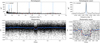 |
Fig. 2 Discovery data of MASCARA-4 b/bRing-1 b. Top left: BLS periodogram of the combined MASCARA and bRing photometry obtained between mid-2017 and the end of 2018. The blue dashed lines represent harmonics of the main periodic signal. Top right: same zoomed-in on the peak in the periodogram, which is located at 0.354 days−1. Bottom left: calibrated MASCARA and bRing data, phase folded to a period of 2.82407 days. The blue dots are binned such that there are nine data points in transit, which comes out to phase steps of ~0.005. The red lineshows the BLS fit on the data. Bottom right: same zoomed-in on the transit event. |
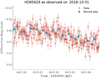 |
Fig. 3 CHAT follow-up observations of MASCARA-4 b. An ingress is clearly seen which is consistent with the ephemeris and transit shape determined from the MASCARA/bRing data. |
3.2 Radial velocity measurements with FIDEOS
We obtained 27 spectra of MASCARA-4 with the FIber Dual Echelle Optical Spectrograph (FIDEOS, Vanzi et al. 2018)mounted on the ESO 1.0 m telescope at La Silla Observatory. FIDEOS has a spectral resolution of 42 000 and covers the wavelength range from 400 to 700 nm. It is stabilised in temperature at the 0.1 K level and uses a secondary fibre illuminated with a ThAr lamp for tracing the instrumental RV drift during a scientific exposure. Fourteen spectra were acquired during UT 24-27 May 2018, while another set of 13 spectra were obtained between UT6 and 21 November 2018. The adopted exposure time for each measurement was 900 seconds, which generated a typical signal-to-noise ratio (S/N) at 5150 Å of 105. FIDEOS data were processed with a dedicated automatic pipeline built using the routines from the CERES package (Brahm et al. 2017). This pipeline performs the frame reductions, the optimal extraction of each spectra, the wavelength calibration, and the instrumental drift correction. Dedicated Interactive Data Language (IDL) procedures were used to derive the RV variations of the target.
To use a cross-correlation template, a detailed synthetic spectrum was computed using the IDL interface SYNPLOT (I. Hubeny, priv. comm.) to the spectrum synthesis program SYNSPEC1, using Kurucz model atmospheres2.
3.3 Doppler-shadow measurements with CHIRON
High-resolution spectroscopic data were taken via the CHIRON on the SMARTS 1.5 m telescope in Chile. MASCARA-4 was observed on UT 25 January 2019 during one of the predicted transits in order to measure the Rossiter-McLaughlin effect, which in combinationwith RV measurements would be an unambiguous signature of the planetary nature of MASCARA-4 b. We obtained a series of 60 spectra, 50 being in-transit and 10 out-of-transit. The spectra were reduced according to the CHIRON pipeline. The start of the transit was missed, and observations continued for around 30 min after the end of the transit.
4 System and stellar parameters
4.1 Photometric transit fitting
The photometric modelling of the transit is performed in a similar way as for MASCARA-1 b (Talens et al. 2018a) and MASCARA-2 b (Talens et al. 2018b). We fit a Mandel & Agol (2002) model to the MASCARA data using a Markov-chain Monte Carlo (MCMC) approach, using the Python codes BATMAN (Kreidberg 2015) and EMCEE (Foreman-Mackey et al. 2013). We assumed a circular orbit (e = 0), as planets with periods of less than six days are known to have negligible eccentricities due to tidal dissipation in the planet (Dobbs-Dixon et al. 2004), and optimised for the fit parameters: the transit epoch TP, the orbital period P, the transit duration T14, the planet-to-star radius ratio p, and the impact parameter b. We use parameters obtained from the discovery BLS algorithm as initial parameters. We fit the uncorrected MASCARA data, including polynomials used to correct instrumental effects (Talens et al. 2018c). For this fit, a linear limb-darkening coefficient of 0.6 was used. The best-fit parameter values come from the median of the output MCMC chains, and the 1σ uncertainties from the 16th and 84th percentiles of the distributions.
Table 2 lists the parameters derived from this model, as well as the reduced chi-square of the data. The reduced chi-square of 1.43 of this fit indicates that the errors are likely underestimated by about 20%, most likely due to minor unreduced instrumental effects in the data. Figure 4 shows the phase-folded photometric light curve of MASCARA-4 b with the best-fit transit model.
Parameters and best-fit values derived from the MASCARA and bRing joint photometric data.
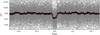 |
Fig. 4 Photometric light curve of MASCARA-4 b, using the best-fit parameters listed in Table 2. The grey points indicate individual data, and the black dots are binned the same as in Fig. 2. The red line shows the photometric model. |
4.2 Radial velocity analysis and planet mass
For the RV analysis we used the 27 FIDEOS spectra. Since the projected equatorial rotation velocity of the star is very high,rotational broadening is the dominant component in the line profiles, resulting in substantial uncertainties on the RV measurements. The individual RV points were phase folded using the best-fit values from photometry, and individual data points taken in sequence on the same night were binned, resulting in seven RV measurements with uncertainties of ~200 m s−1 (see Fig. 5).
A circular orbital solution, with RV amplitude and system velocity as free parameters, was fit to the data. This results formally in a detection of a sinusoidal variation with an amplitude of 310 ± 90 m s−1. Assuming a stellar mass of 1.75 ± 0.05 M⊙ (see Sect. 4.4), this corresponds to a planet mass of 3.1 ± 0.9MJup, well within the planetary regime. It is important to note that this mass measurement is dependent on one particular data point (which shows in the large error in mass), and further RV measurements will be needed to constrain the mass further.
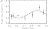 |
Fig. 5 Radial velocity data of MASCARA-4 taken with the FIDEOS spectrograph on the ESO 1m telescope. A marginal sinusoidal variation is detected at 3σ with an amplitude of 310 ± 90 m s−1. Assuming a stellar mass of 1.75 ± 0.05 M⊙, this corresponds to a planet mass of 3.1 ± 0.9 MJup, well within the planetary regime. |
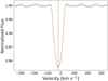 |
Fig. 6 Average CCF for the ten out-of-transit observations with CHIRON. We compute the vsini of this star to be
|

4.3 Doppler-shadow analysis
In order to successfully validate the planetary nature of MASCARA-4 b, a spectroscopic time series during a transit was taken with CHIRON. This observation allows us to establish that a planet-sized dark object transits the bright, fast-spinning star. In addition, the projected spin-orbit angle of the system is determined. For our analysis, cross correlation functions (CCF) were constructed from the reduced CHIRON spectra using the same Kurucz spectral template as used for the RV analysis. In our analysis, we used all 41 orders blueward of 6950 Å, except orders 7, 8, 28, 29, 34, 37, and 38 to avoid the Balmer series and telluric contaminations. The CCF for each observation was constructed by summing the CCF of each individual order, which were subsequently all scaled to the same level.
We first extracted the average out-of-transit CCF of the star, using the last ten observations of the sequence, and the same Kurucz spectral template; see Fig. 6. We fitted a rotationally broadened model (Gray 1976) to this data using an MCMC fitting procedure (from Foreman-Mackay, EMCEE; Foreman-Mackey et al. 2013). We find that the v sin i* =  km s−1, with the errors representing 1−σ error bars on the fit. The systemic velocity is found to be vsys = − 18.31 ± 0.13 km s−1 (1− σ).
In order to extract the Rossiter-McLaughlin information from the data, we followed the “Reloaded” method (Cegla et al. 2016; Bourrier et al. 2017, 2018; Wyttenbach et al. 2017). We first determined the average stellar CCF by taking the mean of theout-of-transit CCFs, corresponding to the last ten observations. We then normalised each CCF by the BLS photometric fit, and subsequently computed the difference between the out-of-transit CCF and each observation.The final residual CCFs are obtained by removing the constant offset. The Doppler shadow of the planetary sized object, coined as MASCARA-4 b, is clearly seen in the data (Fig. 7). We note that the ingress of the transit was missed only marginally. A Gaussian model was fitted to the residual CCFs to determine the RV of the Doppler shadow feature at each epoch during the transit, while the stellar systemic velocity of vsys = − 18.31 ± 0.13 km s−1 was removed from each measurement. For 16 residual CCFs the fit did not converge; this was due to poor S/N or a weaker signal at ingress or egress. Finally, 34 out of the 50 observations in transit had a sufficient velocity precision to be used to constrain the Rossiter-McLaughlin effect and to obtain λ, the projected spin-orbit angle (the addition or removal of the 16 bad velocities does not change our results). To model the residual CCF velocities, we computed the brightness-weighted average rotational velocity behind the planet during each exposure as a function of the transit parameter, the spin-orbit angle, and the stellar velocity field which is given, when assuming a rigid body rotation, by the v sin i* (Cegla et al. 2016).
We decided to perform the next analysis in two steps. In the first step (the unconstrained fit), we assumed Gaussian priors coming from the photometric light curve from MASCARA and bRing for Rp ∕R* and a∕R*, and used a uniform prior for the impact parameter b. We also used uniform priors for λ, veq, i* over their valid ranges. We fitted these six parameters using EMCEE code with 120 walkers and 20000 steps after the burn-in time. In the second step (the constrained fit), we used a Gaussian prior for v sin i* which comes from our spectroscopic fit of  km s−1 from Fig. 6. The only difference between these two fits is our prior on v sin i*. The results of this can be found in Table 3. We note that our results without the v sin i* prior are already quite constraining because the star is a high rotator. Moreover, the measured v sin i* is compatible with the previous spectroscopic measurement, justifying the use of the spectroscopic v sin i* as a prior for our final result.
The resulting fit is shown as a white dotted line in Fig. 7. We find an impact parameter of  and a spin-orbit angle |λ| of
  °. Such an obliquity is set as retrograde (we use the standards present in Addison et al. (2013), with a retrograde orbit being classified as having an obliquity of 112.5° ≤ |λ|≤ 247.5°, and a polar orbit being classified as having anobliquity of 67.5° < |λ| < 112.5°). This makes MASCARA-4 b the brightest known system with a hot Jupiter in a retrograde orbit. The projected orientation of the orbit is shown in the right panel of Fig. 7.
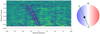 |
Fig. 7 Left: Doppler-shadow measurements on MASCARA-4 b during transit as derived from observations taken with the CHIRON spectrograph on the SMARTS 1.5 m telescope. These consist of 60 mean stellar line profiles from which the average out-of-transit profile is subtracted, showing the movement of the dark planet in front of the fast-rotating star. The black horizontal lines denote t2 and t3 (dashed;the time when the orbiting object starts to ingress and egress) and t1 and t4 (solid; when the orbiting object starts to transit and is no longer transiting) of the transit. Observations started just after t2. The dashed vertical black line represents the systemic velocity of the star, which is set to 0 km s−1. The two vertical white dashed lines indicate the extent of the velocity broadened stellar line profile with a
v sin i* of 46.5 km s−1. The white dotted line represents the best-fit model, corresponding to an impact parameter of
|


Parameters and best-fit values from the CHIRON Rossiter-McLaughlin observations.
4.4 Stellar parameters
4.4.1 Primary star HD 85628 A
HD 85628 is a relatively poorly studied V = 8.19 star in the Carina constellation (ESA 1997), with its only previous reference in SIMBAD being from spectral classification in the Michigan Spectral Survey (A3V; Houk & Cowley 1975). The Gaia DR2 trigonometric parallax for this star (ϖ = 5.8297 ± 0.0318 mas) implies a distance of d = 171.54 ± 0.94 pc, and its astrometric and photometric observables are summarised in Table 4. The optical and near-IR colours of the star are consistent with a A7V (Pickles & Depagne 2010), and this is confirmed via comparison of the observed colours (e.g. Bp−Rp = 0.2548, B−V = 0.20, V −Ks = 0.45) to those of main sequence dwarfs in the table by Pecaut & Mamajek (2013).3 From the Stilism 3D reddening maps of the solar vicinity by Capitanio et al. (2017), we estimate that a star at the position of HD 85628 is predicted to have reddening E(B−V) = 0.020 ± 0.018 mag, which for the standard reddening law (Fiorucci & Munari 2003) translates to an extinction of AV = 0.063 ± 0.056 mag. We discount the large extinction and reddening values quoted in the Gaia DR2 catalogue (Gaia Collaboration 2018) (AG = 0.5012 mag, E(BP−RP) = 0.2580
 mag), which would unphysically require the star to really be a ~A0V star4.
We further constrain the stellar parameters for HD 85628 using the Virtual Observatory SED Analyzer (VOSA)5 and fitting the Hα profile of the star’s CHIRON spectrum. We fit the spectral energy distribution (SED; Fig. 8) of HD 85628 using published photometry from Tycho (BT VT; ESA 1997), APASS (BV; Henden et al. 2016), Gaia DR2 (BpRpG; Gaia Collaboration 2018), DENIS (JK; Epchtein et al. 1994), 2MASS (JHKs; Skrutskie et al. 2006), and WISE (W1W2W3W4; Wright et al. 2010), and fit Kurucz ATLAS9 stellar atmosphere models (Castelli & Kurucz 2003). Given that the star is clearly main sequence and relatively young ( <1 Gyr), we constrain the surfacegravity to be within ±0.5 dex of log g = 4.0 and metallicity within ±0.5 dex of solar, and include the extinction and 1σ uncertainty presented previously as a constraint, but allow the effective temperature to float. We find the best-fit parameters to be for a Kurucz model with Teff, = 7844 K, log g = 4.0, and solar metallicity. We also fitted the shape of the Hα line from the average high-resolution CHIRON spectra with a grid of Kurucz spectra (as used above). While we fail to meaningfully constrain its metallicity and surface gravity in this way, the spectral line shape is consistent with a temperature of 7700 ± 300 K. Based on these independentanalyses, we adopt Teff ≃ 7800 ± 200 K. We note that this is somewhat cooler than expected given the A3V classification by Houk & Cowley (1975), since typical A3V stars have Teff ≃ 8550 K (Pecaut & Mamajek 2013), however we cannot reconcile such a hot temperature given the available data, leading us to believe that the initial classification was incorrect, and that this star is in fact an A7V star. The best-fit luminosity to SED fit using the VO Sed Analyzer (VOSA) tool, and adopting the distance based on the Gaia DR2 trigonometric parallax, is L = 12.23 ± 0.0655 L⊙ or log (L∕L⊙) ≃ 1.087 ± 0.023 dex. For the adopted effective temperature, this implies that HD 85628 has a radius of 1.92 ± 0.11 R⊙ 6.
The duration of the transit provides an estimate of the average density of the host star, assuming a circular orbit and providing that the impact parameter is well known. The latter is very well constrained (b =  ) by the Doppler shadow measurements, with the T14 transit duration measured to be 0.165 ± 0.004 days. This implies that if the impact parameter were zero, the transit duration would be
 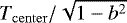 = 0.175 ± 0.005 days, corresponding to the planet travelling over a distance of 2(R* + Rp) = 2.16 ± 0.006R*. By feeding this into Kepler’s third law, we obtain a mean stellar density of 0.41 ± 0.04 g cm−3 (0.29 ± 0.03 ρ⊙).
Interpolating the solar metallicity evolutionary tracks and isochrones of Bertelli et al. (2009) using our adopted effective temperature and luminosity, one predicts a mass of 1.75 M⊙, an age of 0.82 Gyr, and a surface gravity of log g = 4.11. We use the online PARAM 1.1 interface7 to provide Bayesian estimates of stellar parameters based on the HR diagram position for HD 85628. Using the evolutionary tracks of Girardi et al. (2000), and adopting AV = 0.07 and metallicity within ±0.1 dex of solar, PARAM predicts an isochronal age of 0.7 ± 0.2 Gyr, a mass of 1.753 ± 0.044 M⊙, and log g = 4.09 ± 0.05. Given the empirical mass–luminosity relationship for well-measured main sequence stars by Eker et al. (2015), our adopted L for HD 85628 would predict a mass of 1.78 ± 0.11 M⊙. Based on these estimates, we adopt a mass of 1.75 ± 0.05 M⊙, log g ≃ 4.10 ± 0.05, and an age of 0.8 Gyr. The predicted density (0.252 ± 0.045ρ⊙) compares well to that predicted by the transit and Kepler’s third law (0.29 ± 0.03ρ⊙).
Stellar parameters.
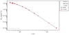 |
Fig. 8 Spectral energy distribution for HD 85628 generated using VOSA. Photometry from Tycho, Gaia DR2, APASS, DENIS, 2MASS, and WISE are plotted (for references, see Sect. 4.4). Overlain is a synthetic stellar spectrum from Castelli & Kurucz (2003) for Teff = 7750 K with log g = 3.5, solar metallicity, AV = 0.07, and corresponding to bolometric luminosity 12.23 ± 0.655 L⊙ (adopting the distance implied by the inverse of the Gaia DR2 trigonometric parallax). |
4.4.2 Stellar companion HD 85628 B
The Gaia DR2 catalogue shows that the star HD 85628 (Gaia DR2 5245968236116294016) has a companion, which we designate HD 85628 B (Gaia DR2 5245968236111767424), previously unreported in the Washington Double Star Catalog (Mason et al. 2001). The G-band magnitude of the companion (14.0490 ± 0.0047) is 5.875 mag fainter than that of HD 85628, and it lies 4336.21 ± 0.06 mas away at position angle 224.938° (ICRS, epoch 2015.5), corresponding to a projected separation of ~736 AU. The pair clearly demonstrate common proper motion and parallax as seen in Table 4. The proper motion of B with respect to A is Δμα, Δμδ = -0.20 ± 0.09, +2.15 ± 0.08 mas yr−1, which at the weighted mean distance (170.0 ± 0.7 pc) corresponds to a tangential (projected orbital motion) velocity of B with respect to A of 1.74 ± 0.09 km s−1.
Gaia DR2 Bp and Rp photometry for HD 85628 B are likely corrupted given the large value of E(BR/RP) of 2.325, which far exceeds the threshold for reliable photometry for stars of similar Bp –Rp colour determined by Evans et al. (2018). Besides Gaia DR1 and DR2, the only pre-Gaia catalogue that has an entry for HD 85628 B is USNO-B1.0 (USNO B1.0-0238-0154014; Monet et al. 2003). We have limited colour data and no spectral data for HD 85628 B, however from its inferred absolute magnitude MG ≃ 7.9, it would compare well to low-mass solar neighbours like η Cas B (K7V: MG = 7.89) or HD 79210 (M0V; MG = 7.96). We predict HD 85628 B to be a ~K8V star with a mass of ~0.6 M⊙.
For component masses of 1.75 M⊙ and 0.6 M⊙, and fiducially setting the observed separation 736 AU as a first estimate of the semi-major axis and assuming e = 0, one would predict an orbital period of ~13 000 yr and relative orbital motion of 1.68 km s−1. This is remarkably similar to the observed difference in tangential motion (1.74 ± 0.09 km s−1) observed forA and B using the Gaia DR2 astrometry. This calculation also further strengthens the argument that the two stars are likely to be a bound pair.
5 Discussion and conclusion
The parameters describing the MASCARA-4 b/bRing-1 b system are shown in Table 5. We find that MASCARA-4 b/bRing-1 b orbits its host star with a period of 2.82406 ± 0.00003 days at a distance of 0.047 ± 0.004 AU. It has a radius of  RJup with a mass of 3.1 ± 0.9 MJup. The planet equilibrium temperatureis 2100 ± 100 K, assuminga Bond albedo of zero.
The planet is in a retrograde orbit, |λ| = °, around its host, a hot (Teff =7800 ± 200 K) A-type star. Together they make up the brightest system known to date with a planet in a retrograde orbit (112.5° ≤ |λ|≤ 247.5°, following Addison et al. 2013), and currently one of only 15 known retrograde systems according to the TEPCat catalogue (Southworth 2011); see Fig. 9. This is contrasted with 18 exoplanets in known polar orbits (67.5° < |λ| < 112.5°), with 219 currently known exoplanets with derived obliquities. As found in earlier work (Albrecht et al. 2012; Schlaufman 2010; Winn et al. 2010), hot Jupiters orbiting early-type stars have a significantly higher probability of being in a polar or retrograde orbit. Currently, 0.081% of planets orbiting stars with Teff < 6300 K are found in such orbits, while this is 39.6% for planets orbiting stars with Teff > 6300 K. It is unclear how such misalignment could result from early planet–disk interactions, and it is more likely that this is caused by Kozai–Lidovoscillations with a more distant companion. Indeed, we find HD 85628 to have a late-type companion (likely a ~K8 dwarf), currently at a projected distance of ~736 AU. It is yet unclear why hot Jupiters orbiting early-type stars are more likely to be misaligned. It is possible that their formation mechanism is different from current models. However, it has also been suggested that the fact that outer layers of lower-mass stars are convective, which shortens the timescale of orbital re-alignment (Winn et al. 2010), erasing the evidence of the Kozai–Lidov effect.
The Doppler shadow measurement only determined the projected spin-orbit angle, while the real spin-orbit angle is degenerate with the stellar inclination. The v sin i* of the host star is relatively low ( km s−1) for its spectral type (Zorec & Royer 2012), implying that the true inclination may be very different, making its true de-projected orbit either more retrograde, or more polar − depending on the value of the inclinationangle. Compared to v sin i values for dwarf stars of the same subtype from Zorec & Royer (2012), the star’s v sin i would place it in the 4th percentile among A7V stars (our estimated spectral type), or 7th percentile among A3V stars (Houk type). It is unlikely that the star has such a low rotational velocity, but this is not unheard of for such stars (Zorec & Royer 2012).
The brightness of the host star, combined with the short orbital period and high planet temperature, make MASCARA-4 b an excellent candidate for follow-up atmospheric studies, reminiscent of WASP-33 b (Collier Cameron et al. 2010). The hottest gas giant planets are found to have unique atmospheric features. The hottest of all, KELT-9 b (Gaudi et al. 2017; Yan & Henning 2018), exhibits an optical transmission spectrum rich in metallic atoms and ions such as iron and titanium (Hoeijmakers et al. 2018), while it shows strong Hα absorption originating from a halo of escaping hydrogen gas. A planet like WASP-33 b shows a thermal dayside spectrum dominated by TiO emission lines, indicative of a strong thermal inversion (Nugroho et al. 2017). Detailed atmospheric observations of a significant sample of the hottest Jupiters are required to understand how these features depend on the planet and possible host star properties, and to understand the underlying physical and chemical mechanisms. In any case, these systems will be the easiest to study with current instruments, and with future observatories such as the James Webb Space Telescope and the ground-based extremely large telescopes. The NASA TESS satellite covered this target in Sectors 10 and 11, which may constrain the secondary eclipse and phase curve of the planet, and thus its dayside temperature and global circulation.
Parameters describing the MASCARA-4 b/bRing-1 b system.
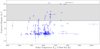 |
Fig. 9 All currently known exoplanets with measured projected obliquities, as taken from the TEPCat catalogue (Southworth 2011). MASCARA-4 b is shown as a blue star. This further emphasises the trend that those planets orbiting hot stars have a larger probability of being in a mis-aligned orbit. The grey shaded regions denote what is considered to be a retrograde planet, with projected obliquity 112.5° ≤|λ|≤ 247.5°. |
Acknowledgements
I.S. acknowledges support from a NWO VICI grant (639.043.107). This project has received funding from the European Research Council (ERC) under the European Union’s Horizon 2020 research and innovation programme (grant agreement nr. 694513). E.E.M. and S.N.M. acknowledge support from the NASA NExSS programme. SNM is a US Department of Defense SMART scholar sponsored by the U.S. Navy through NIWC-Atlantic. E.E.M. acknowledges support from the NASA NExSS program and a JPL RT&D award. A.W. acknowledges the support of the SNSF by the grant number P2GEP2 178191. L.V. acknowledges the support of CONICYT Project Fondecyt n. 1171364. Part of this research was carried out at the Jet Propulsion Laboratory, California Institute of Technology, under a contract with the National Aeronautics and Space Administration. This work has made use of data from the European Space Agency (ESA) mission Gaia (https://www.cosmos.esa.int/gaia), processed by the Gaia Data Processing and Analysis Consortium (DPAC, https://www.cosmos.esa.int/web/gaia/dpac/consortium). This research has made use of the SIMBAD database, operated at CDS, Strasbourg, France. This research has made use of the VizieR catalogue access tool, CDS, Strasbourg, France. We have benefited greatly from the publicly available programming language Python, including the numpy (Oliphant 2006), matplotlib (Hunter 2007), pyfits, scipy (Jones et al. 2001) and h5py (Collette 2008) packages. Pyfits is a product of the Space Telescope Science Institute, which is operated by AURA for NASA. The authors would like to acknowledge the support staff at both the South African Astronomical Observatory and Siding Spring Observatory for keeping both bRing stations maintained and running, and the ESO La Silla TMES staff for their support with MASCARA-S.
References
- Addison, B. C., Tinney, C. G., Wright, D. J., et al. 2013, ApJ, 774, L9 [NASA ADS] [CrossRef] [Google Scholar]
- Albrecht, S., Winn, J. N., Johnson, J. A., et al. 2012, ApJ, 757, 18 [NASA ADS] [CrossRef] [Google Scholar]
- Bakos, G., Noyes, R. W., Kovács, G., et al. 2004, PASP, 116, 266 [NASA ADS] [CrossRef] [Google Scholar]
- Barge, P., Baglin, A., Auvergne, M., et al. 2008, A&A, 482, L17 [NASA ADS] [CrossRef] [EDP Sciences] [Google Scholar]
- Batalha, N. M. 2014, Proc. Natl. Acad. Sci., 111, 12647 [NASA ADS] [CrossRef] [Google Scholar]
- Bertelli, G., Nasi, E., Girardi, L., & Marigo, P. 2009, A&A, 508, 355 [NASA ADS] [CrossRef] [EDP Sciences] [Google Scholar]
- Borucki, W. J., Koch, D., Basri, G., et al. 2010, Science, 327, 977 [NASA ADS] [CrossRef] [PubMed] [Google Scholar]
- Bouchy, F., Udry, S., Mayor, M., et al. 2005, A&A, 444, L15 [NASA ADS] [CrossRef] [EDP Sciences] [Google Scholar]
- Bourrier, V., Cegla, H. M., Lovis, C., & Wyttenbach, A. 2017, A&A, 599, A33 [NASA ADS] [CrossRef] [EDP Sciences] [Google Scholar]
- Bourrier, V., Lovis, C., Beust, H., et al. 2018, Nature, 553, 477 [NASA ADS] [CrossRef] [Google Scholar]
- Brahm, R., Jordán, A., & Espinoza, N. 2017, PASP, 129, 034002 [NASA ADS] [CrossRef] [Google Scholar]
- Capitanio, L., Lallement, R., Vergely, J. L., Elyajouri, M., & Monreal-Ibero, A. 2017, A&A, 606, A65 [NASA ADS] [CrossRef] [EDP Sciences] [Google Scholar]
- Castelli, F., & Kurucz, R. L. 2003, IAU Symp., 210, A20 [Google Scholar]
- Cegla, H. M., Lovis, C., Bourrier, V., et al. 2016, A&A, 588, A127 [NASA ADS] [CrossRef] [EDP Sciences] [Google Scholar]
- Charbonneau, D., Brown, T. M., Latham, D. W., & Mayor, M. 2000, ApJ, 529, L45 [NASA ADS] [CrossRef] [PubMed] [Google Scholar]
- Collette, A. 2008, HDF5 for Python, [Online; accessed] [Google Scholar]
- Collier Cameron, A., Guenther, E., Smalley, B., et al. 2010, MNRAS, 407, 507 [NASA ADS] [CrossRef] [Google Scholar]
- Cutri, R. M., et al. 2012, VizieR Online Data Catalog: II/311 [Google Scholar]
- Dawson, R. I., & Johnson, J. A. 2018, ARA&A, 56, 175 [NASA ADS] [CrossRef] [Google Scholar]
- Dobbs-Dixon, I., Lin, D. N. C., & Mardling, R. A. 2004, ApJ, 610, 464 [NASA ADS] [CrossRef] [Google Scholar]
- Eker, Z., Soydugan, F., Soydugan, E., et al. 2015, AJ, 149, 131 [NASA ADS] [CrossRef] [Google Scholar]
- Epchtein, N., de Batz, B., Copet, E., et al. 1994, Ap&SS, 217, 3 [NASA ADS] [CrossRef] [Google Scholar]
- ESA, ed. 1997, The Hipparcos and Tycho catalogues. Astrometric and Photometric Star Catalogues Derived from the ESA Hipparcos Space Astrometry Mission (Noordwijk: ESA SP), 1200 [Google Scholar]
- Espinoza, N., Hartman, J. D., Bakos, G. A., et al. 2019, AJ, 158, 63 [NASA ADS] [CrossRef] [Google Scholar]
- Evans, D. W., Riello, M., De Angeli, F., et al. 2018, A&A, 616, A4 [NASA ADS] [CrossRef] [EDP Sciences] [Google Scholar]
- Fiorucci, M., & Munari, U. 2003, A&A, 401, 781 [NASA ADS] [CrossRef] [EDP Sciences] [Google Scholar]
- Foreman-Mackey, D., Hogg, D. W., Lang, D., & Goodman, J. 2013, PASP, 125, 306 [CrossRef] [Google Scholar]
- Gaia Collaboration (Brown, A. G. A., et al.) 2018, A&A, 616, A1 [NASA ADS] [CrossRef] [EDP Sciences] [Google Scholar]
- Gandolfi, D., Collier Cameron, A., Endl, M., et al. 2012, A&A, 543, L5 [NASA ADS] [CrossRef] [EDP Sciences] [Google Scholar]
- Gaudi, B. S., Stassun, K. G., Collins, K. A., et al. 2017, Nature, 546, 514 [NASA ADS] [Google Scholar]
- Girardi, L., Bressan, A., Bertelli, G., & Chiosi, C. 2000, A&AS, 141, 371 [NASA ADS] [CrossRef] [EDP Sciences] [Google Scholar]
- Gray, D. F. 1976, The Observation and Analysis of Stellar Photospheres (Cambridge: Cambridge University Press) [Google Scholar]
- Hartman, J. D., Bakos, G. A., Bayliss, D., et al. 2019, AJ, 157, 55 [NASA ADS] [CrossRef] [Google Scholar]
- Henden, A. A., Templeton, M., Terrell, D., et al. 2016, VizieR Online Data Catalog: II/336 [Google Scholar]
- Hjorth, M., Albrecht, S., Talens, G. J. J., et al. 2019, A&A, 631, A76 [NASA ADS] [CrossRef] [EDP Sciences] [Google Scholar]
- Hoeijmakers, H. J., Ehrenreich, D., Heng, K., et al. 2018, Nature, 560, 453 [NASA ADS] [CrossRef] [Google Scholar]
- Houk, N., & Cowley, A. P. 1975, University of Michigan Catalogue of Two-dimensional Spectral Types for the HD Stars (Michigan: University of Michigan) 1 [Google Scholar]
- Hunter, J. D. 2007, Comput. Sci. Eng., 9, 90 [NASA ADS] [CrossRef] [Google Scholar]
- Jones, E., Oliphant, T., Peterson, P., et al. 2001, SciPy: Open source scientific tools for Python, [Online; accessed] [Google Scholar]
- Jordán, A., Brahm, R., Espinoza, N., et al. 2019, AJ, 157, 100 [NASA ADS] [CrossRef] [Google Scholar]
- Kalas, P., Zwintz, K., Kenworthy, M., et al. 2019, AAS Meeting Abstracts, 233, 218.03 [Google Scholar]
- Kenworthy, M. 2017, Nat. Astron., 1, 0099 [NASA ADS] [CrossRef] [Google Scholar]
- Kovács, G., Zucker, S., & Mazeh, T. 2002, A&A, 391, 369 [NASA ADS] [CrossRef] [EDP Sciences] [Google Scholar]
- Kreidberg, L. 2015, PASP, 127, 1161 [NASA ADS] [CrossRef] [Google Scholar]
- Lammer, H., Selsis, F., Ribas, I., et al. 2003, ApJ, 598, L121 [NASA ADS] [CrossRef] [Google Scholar]
- Latham, D. W., Mazeh, T., Stefanik, R. P., Mayor, M., & Burki, G. 1989, Nature, 339, 38 [NASA ADS] [CrossRef] [Google Scholar]
- Mandel, K., & Agol, E. 2002, ApJ, 580, L171 [NASA ADS] [CrossRef] [Google Scholar]
- Mason, B. D., Wycoff, G. L., Hartkopf, W. I., Douglass, G. G., & Worley, C. E. 2001, AJ, 122, 3466 [Google Scholar]
- Mayor, M., & Queloz, D. 1995, Nature, 378, 355 [Google Scholar]
- McCullough, P. R., Stys, J. E., Valenti, J. A., et al. 2005, PASP, 117, 783 [NASA ADS] [CrossRef] [Google Scholar]
- Mellon, S. N., Stuik, R., Kenworthy, M., et al. 2019a, AAS Meeting Abstracts, 233, 140.22 [Google Scholar]
- Mellon, S. N., Mamajek, E. E., Zwintz, K., et al. 2019b, ApJ, 870, 36 [NASA ADS] [CrossRef] [Google Scholar]
- Mellon, S. N., Mamajek, E. E., Stuik, R., et al. 2019c, ApJS, 244, 15 [NASA ADS] [CrossRef] [Google Scholar]
- Monet, D. G., Levine, S. E., Canzian, B., et al. 2003, AJ, 125, 984 [NASA ADS] [CrossRef] [Google Scholar]
- Nugroho, S. K., Kawahara, H., Masuda, K., et al. 2017, AJ, 154, 221 [NASA ADS] [CrossRef] [Google Scholar]
- Oliphant, T. 2006, NumPy: a Guide to NumPy (USA: Trelgol Publishing) [Google Scholar]
- Pecaut, M. J.,& Mamajek, E. E. 2013, ApJS, 208, 9 [NASA ADS] [CrossRef] [Google Scholar]
- Pepper, J., Pogge, R. W., DePoy, D. L., et al. 2007, PASP, 119, 923 [NASA ADS] [CrossRef] [Google Scholar]
- Pickles, A., & Depagne, É. 2010, PASP, 122, 1437 [NASA ADS] [CrossRef] [Google Scholar]
- Pollacco, D. L., Skillen, I., Collier Cameron, A., et al. 2006, PASP, 118, 1407 [NASA ADS] [CrossRef] [Google Scholar]
- Reis, W., Corradi, W., de Avillez, M. A., & Santos, F. P. 2011, ApJ, 734, 8 [NASA ADS] [CrossRef] [Google Scholar]
- Ricker, G. R., Winn, J. N., Vanderspek, R., et al. 2015, J. Astron. Telesc. Instrum. Syst., 1, 014003 [NASA ADS] [CrossRef] [Google Scholar]
- Schlaufman, K. C. 2010, ApJ, 719, 602 [NASA ADS] [CrossRef] [Google Scholar]
- Skrutskie, M. F., Cutri, R. M., Stiening, R., et al. 2006, AJ, 131, 1163 [NASA ADS] [CrossRef] [Google Scholar]
- Snellen, I. A. G., Stuik, R., Navarro, R., et al. 2012, Proc. SPIE, 8444, 84440I [CrossRef] [Google Scholar]
- Southworth, J. 2011, MNRAS, 417, 2166 [NASA ADS] [CrossRef] [Google Scholar]
- Stuik, R., Bailey, J. I., Dorval, P., et al. 2017, A&A, 607, A45 [NASA ADS] [CrossRef] [EDP Sciences] [Google Scholar]
- Sullivan, P. W., Winn, J. N., Berta-Thompson, Z. K., et al. 2015, ApJ, 809, 77 [NASA ADS] [CrossRef] [Google Scholar]
- Szentgyorgyi, A. H., & Furész, G. 2007, Rev. Mex. Astron. Astrofis., 27, 129 [Google Scholar]
- Talens, G. J. J., Spronck, J. F. P., Lesage, A. L., et al. 2017, A&A, 601, A11 [NASA ADS] [CrossRef] [EDP Sciences] [Google Scholar]
- Talens, G. J. J., Albrecht, S., Spronck, J. F. P., et al. 2018a, A&A, 613, C2 [CrossRef] [EDP Sciences] [Google Scholar]
- Talens, G. J. J., Justesen, A. B., Albrecht, S., et al. 2018b, A&A, 612, A57 [NASA ADS] [CrossRef] [EDP Sciences] [Google Scholar]
- Talens, G. J. J., Deul, E. R., Stuik, R., et al. 2018c, A&A, 619, A154 [NASA ADS] [CrossRef] [EDP Sciences] [Google Scholar]
- Vanzi, L., Zapata, A., Flores, M., et al. 2018, MNRAS, 477, 5041 [NASA ADS] [CrossRef] [Google Scholar]
- Vidal-Madjar, A., Lecavelier des Etangs, A., Désert, J.-M., et al. 2003, Nature, 422, 143 [NASA ADS] [CrossRef] [PubMed] [Google Scholar]
- Winn, J. N., Fabrycky, D., Albrecht, S., & Johnson, J. A. 2010, ApJ, 718, L145 [NASA ADS] [CrossRef] [Google Scholar]
- Wright, E. L., Eisenhardt, P. R. M., Mainzer, A. K., et al. 2010, AJ, 140, 1868 [NASA ADS] [CrossRef] [Google Scholar]
- Wright, J. T., Marcy, G. W., Howard, A. W., et al. 2012, ApJ, 753, 160 [NASA ADS] [CrossRef] [Google Scholar]
- Wyttenbach, A., Lovis, C., Ehrenreich, D., et al. 2017, A&A, 602, A36 [NASA ADS] [CrossRef] [EDP Sciences] [Google Scholar]
- Yan, F., & Henning, T. 2018, Nat. Astron., 2, 714 [NASA ADS] [CrossRef] [Google Scholar]
- Zorec, J., & Royer, F. 2012, A&A, 537, A120 [NASA ADS] [CrossRef] [EDP Sciences] [Google Scholar]
See updated table at: http://www.pas.rochester.edu/~emamajek/EEM_dwarf_UBVIJHK_colors_Teff.txt.
Unusually high reddenings and extinctions from Apsis-Priam appear to be a feature of the Gaia DR2 catalog. The well-characterized stars with SIMBAD entries with DR2 parallaxes that place them within 10 pc have a median extinction of AG ≃ 0.24 mag (mean 0.34, standard deviation 0.39 mag) in the Gaia DR2. These stars should all comfortably lie within the Local Bubble with near-zero extinction (Reis et al. 2011).
VOSA 6.0: http://svo2.cab.inta-csic.es/theory/vosa/.
Adopting IAU 2015 nominal solar values L⊙ = 3.828 × 1026 W and R⊙ = 695 700 km.
All Tables
Parameters and best-fit values derived from the MASCARA and bRing joint photometric data.
All Figures
|
Fig. 1 Global view of the MASCARA/bRing network. The two MASCARA instruments (white squares) are located in La Silla, Chile, and La Palma, the Canary Islands, Spain, respectively. The two bRing instruments (yellow squares) are located in Sutherland, South Africa, and Coonabarabran, Australia. At any given time, at least one instrument in the southern hemisphere is observing, weather permitting. |
| In the text | |
|
Fig. 2 Discovery data of MASCARA-4 b/bRing-1 b. Top left: BLS periodogram of the combined MASCARA and bRing photometry obtained between mid-2017 and the end of 2018. The blue dashed lines represent harmonics of the main periodic signal. Top right: same zoomed-in on the peak in the periodogram, which is located at 0.354 days−1. Bottom left: calibrated MASCARA and bRing data, phase folded to a period of 2.82407 days. The blue dots are binned such that there are nine data points in transit, which comes out to phase steps of ~0.005. The red lineshows the BLS fit on the data. Bottom right: same zoomed-in on the transit event. |
| In the text | |
|
Fig. 3 CHAT follow-up observations of MASCARA-4 b. An ingress is clearly seen which is consistent with the ephemeris and transit shape determined from the MASCARA/bRing data. |
| In the text | |
|
Fig. 4 Photometric light curve of MASCARA-4 b, using the best-fit parameters listed in Table 2. The grey points indicate individual data, and the black dots are binned the same as in Fig. 2. The red line shows the photometric model. |
| In the text | |
|
Fig. 5 Radial velocity data of MASCARA-4 taken with the FIDEOS spectrograph on the ESO 1m telescope. A marginal sinusoidal variation is detected at 3σ with an amplitude of 310 ± 90 m s−1. Assuming a stellar mass of 1.75 ± 0.05 M⊙, this corresponds to a planet mass of 3.1 ± 0.9 MJup, well within the planetary regime. |
| In the text | |
|
Fig. 6 Average CCF for the ten out-of-transit observations with CHIRON. We compute the vsini of this star to be
|
| In the text | |
|
Fig. 7 Left: Doppler-shadow measurements on MASCARA-4 b during transit as derived from observations taken with the CHIRON spectrograph on the SMARTS 1.5 m telescope. These consist of 60 mean stellar line profiles from which the average out-of-transit profile is subtracted, showing the movement of the dark planet in front of the fast-rotating star. The black horizontal lines denote t2 and t3 (dashed;the time when the orbiting object starts to ingress and egress) and t1 and t4 (solid; when the orbiting object starts to transit and is no longer transiting) of the transit. Observations started just after t2. The dashed vertical black line represents the systemic velocity of the star, which is set to 0 km s−1. The two vertical white dashed lines indicate the extent of the velocity broadened stellar line profile with a
v sin i* of 46.5 km s−1. The white dotted line represents the best-fit model, corresponding to an impact parameter of
|
| In the text | |
|
Fig. 8 Spectral energy distribution for HD 85628 generated using VOSA. Photometry from Tycho, Gaia DR2, APASS, DENIS, 2MASS, and WISE are plotted (for references, see Sect. 4.4). Overlain is a synthetic stellar spectrum from Castelli & Kurucz (2003) for Teff = 7750 K with log g = 3.5, solar metallicity, AV = 0.07, and corresponding to bolometric luminosity 12.23 ± 0.655 L⊙ (adopting the distance implied by the inverse of the Gaia DR2 trigonometric parallax). |
| In the text | |
|
Fig. 9 All currently known exoplanets with measured projected obliquities, as taken from the TEPCat catalogue (Southworth 2011). MASCARA-4 b is shown as a blue star. This further emphasises the trend that those planets orbiting hot stars have a larger probability of being in a mis-aligned orbit. The grey shaded regions denote what is considered to be a retrograde planet, with projected obliquity 112.5° ≤|λ|≤ 247.5°. |
| In the text | |
Current usage metrics show cumulative count of Article Views (full-text article views including HTML views, PDF and ePub downloads, according to the available data) and Abstracts Views on Vision4Press platform.
Data correspond to usage on the plateform after 2015. The current usage metrics is available 48-96 hours after online publication and is updated daily on week days.
Initial download of the metrics may take a while.