| Issue |
A&A
Volume 634, February 2020
|
|
|---|---|---|
| Article Number | A38 | |
| Number of page(s) | 7 | |
| Section | Extragalactic astronomy | |
| DOI | https://doi.org/10.1051/0004-6361/201936586 | |
| Published online | 03 February 2020 | |
Orientation of the crescent image of M 87*
Nicolaus Copernicus Astronomical Center, Polish Academy of Sciences, Bartycka 18, 00-716 Warsaw, Poland
e-mail: This email address is being protected from spambots. You need JavaScript enabled to view it.
Received:
27
August
2019
Accepted:
30
December
2019
Abstract
The first image of the black hole (BH) M 87* obtained by the Event Horizon Telescope (EHT) has the shape of a crescent extending from the E to WSW position angles, while the observed direction of the large-scale jet is WNW. Images based on numerical simulations of BH accretion flows suggest that on average the projected BH spin axis should be oriented SSW. We explore highly simplified toy models for geometric distribution and kinematics of emitting regions in the Kerr metric, perform ray tracing to calculate the corresponding images, and simulate their observation by the EHT to calculate the corresponding visibilities and closure phases. We strictly assume that (1) the BH spin vector is fixed to the jet axis, (2) the emitting regions are stationary and symmetric with respect to the BH spin, and that (3) the emissivities are isotropic in the local rest frames. Emission from the crescent sector between SSE and WSW can be readily explained in terms of an equatorial ring with either circular or plunging geodesic flows, regardless of the value of BH spin. In the case of plane-symmetric polar caps with plunging geodesic flows, the dominant image of the cap located behind the BH is sensitive to the angular momentum of the emitter. Within the constraints of our model, we have not found a viable explanation for the observed brightness of the ESE sector. Most likely, the ESE “hotspot” has been produced by a non-stationary localised perturbation in the inner accretion flow. Alternatively, it could result from locally anisotropic synchrotron emissivities. Multi-epoch and polarimetric results from the EHT will be essential to verify the theoretically expected alignment of the BH spin with the large-scale jet.
Key words: black hole physics / galaxies: active / galaxies: individual: M 87 / gravitation / relativistic processes
© ESO 2020
1. Introduction
The Event Horizon Telescope (EHT) collaboration presented the first resolved image of a photon ring surrounding the supermassive black hole (BH) dubbed M 87* (EHT Collaboration 2019a). The image obtained at a wavelength of λ = 1.3 mm and an angular resolution of ≃20 μas can be best described as an asymmetric crescent of ≃42 μas in diameter with brightness enhanced on the southern side (EHT Collaboration 2019b), or more precisely, for position angles in the range PA ∈ [70° :270° ], that is, ENE–W (EHT Collaboration 2019c, Fig. 27). On the other hand, interferometric observations at longer wavelengths reveal a well-known relativistic jet: at 3.5 mm wavelength the jet collimation and acceleration zone can be probed up to ∼1 mas (Hada et al. 2016; Kim et al. 2018); at 7 mm wavelength mildly superluminal motions can be traced up to ≃6 mas (Mertens et al. 2016; Walker et al. 2018). The jet is directed at the mean position angle of PAjet ≃ 288° (WNW), and this projected direction has been stable over decades of observations.
The EHT image of M 87* has been compared with ray-traced images obtained from an extensive library of general relativistic magnetohydrodynamical (GRMHD) simulations of geometrically thick accretion onto BHs of various spins (EHT Collaboration 2019d). The enhanced brightness on the southern side of the ring has been interpreted as resulting from the Doppler beaming of mildly relativistic plasma flow that is approaching the observer. A sense of rotation for the BH (rather than for the large-scale accretion flow) can be deduced from this as clockwise (CW; corresponding to the observer inclination angle with respect to the BH spin i > 90°). However, the projected orientations of the BH spin vectors – obtained by rotating the simulated images to minimise the difference from the observed image – were found to span a range of PABH ≃ 150° −280°, with the mean value of ≃205° and standard deviation of ≃55° (SSE–W; top panels of Fig. 9 in EHT Collaboration 2019d). The mean offset from PAjet is ≃80° CW, which is equivalent to ∼1.5σ. The predictions of GRMHD simulations specifically tailored to the case of M 87 are that the major axis of the bright part of the ring should be oriented parallel to the projected jet axis (Dexter et al. 2012; Mościbrodzka et al. 2016; Davelaar et al. 2019).
There are strong arguments to support the assumption that relativistic jets should be directed along the BH spin axis – the leading scenario for launching jets is the Blandford-Znajek mechanism (Blandford & Znajek 1977). Numerical simulations demonstrated the robustness of jet alignment even for flipping BH spins (McKinney et al. 2013), and there is no evidence for jet precession in the particular case of M 87 (see Sect. 7.3.(2) in EHT Collaboration 2019d).
In the GRMHD simulations of accretion-jet systems (EHT Collaboration 2019d), the synchrotron emission is produced mainly in the accreting torus or in the outer jet funnel, but not in the polar jet regions. Emission from the polar regions requires additional physical mechanisms of energy dissipation beyond the regime of ideal magnetohydrodynamics (MHD). In particular, these regions could be related to particle-starved gaps in the BH magnetospheres that have been suggested as the sites of very-high-energy gamma ray emission (e.g. Levinson & Rieger 2011; Broderick & Tchekhovskoy 2015; Katsoulakos & Rieger 2018) that has indeed been observed in M 87 and found to be variable on a timescale of days (e.g. Aharonian et al. 2006; Abramowski et al. 2012). The polar regions could also be related to the lamppost model for the origin of hard X-ray emission in active galactic nuclei (AGNs) and X-ray binaries (e.g. Martocchia & Matt 1996; Miniutti & Fabian 2004). The first kinetic simulations of BH magnetospheres with pair creation demonstrate the formation of charge gaps at intermediate latitudes for low enough rates of particle supply (Parfrey et al. 2019). For these reasons, we find it particularly important to include in our study a simplified case of polar caps.
In this letter, we consider highly simplified (stationary, axisymmetric) toy models for the distribution of emitting regions around the BH M 87*, and we ray trace the corresponding images in the Kerr metric in the limit of optically thin emission with uniform fluid-frame emissivity. We fix the BH spin axis at a position angle of PAjet = 288° and inclination of i = 162°. We assume that the emission process is isotropic in local rest frames, and we consider the effect of Doppler beaming due to azimuthal and radial motions of the emitting fluid. We find that our model can naturally explain a section of the crescent image that extends between SSE and WSW position angles, but cannot explain the emission observed in the ESE sector.
2. Methods
We perform ray tracing of scalar radiation in the Kerr metric for BH mass M and spin a (G = 1 = c),
 (1)
(1)
using the Boyer-Lindquist coordinates xμ = (t, r, θ, ϕ) and employing a newly developed numerical code. We integrate the null geodesics xμ(λ) over the affine parameter dλ = dt/pt, with the four-momentum pμ = dxμ/dλ, starting from a stationary observer of position  and four-velocity
  . We perform first-order explicit integration backward in time, with an adaptive time step of dt ∝ r. The integration involves four constants: asymptotic energy E, asymptotic angular momentum L, Carter constant Q, and square of the four-momentum pμpμ = 0 (e.g. Bardeen et al. 1972; Sikora 1979). Integration is interrupted either when the photon falls onto the BH (pt ≥ 103) or when the photon escapes (r > robs).
The emitting regions are assumed to be optically thin with uniform isotropic emissivities with power-law spectrum  of spectral index α in their local rest frames. We adopt a spectral index α = 0.5, and we checked that varying α has little effect on the resulting image. The emission mechanism is not specified, and no absorption of radiation is considered. The emitters are allowed to be in motion relative to the local stationary observers with radial velocities βr = dr/dt and angular velocities Ω = dϕ/dt; hence their four-velocities are
  . From the covariant radiative transfer equation dλ(Iν/ν3) = jν/ν2 (e.g. Mościbrodzka & Gammie 2018), for every geodesic 𝒢 that intersects an emitting region 𝒮, the observed intensity is integrated as being proportional to Iν, obs ∝ ∫𝒢 ∩ 𝒮dλ g2 + α, where
 ![Mathematical equation: $ g = [p_\mu(\lambda_{\rm obs}) u_{\rm obs}^\mu] / [p_\mu(\lambda_{\rm em}) u_{\rm em}^\mu] $](/articles/aa/full_html/2020/02/aa36586-19/aa36586-19-eq6.gif) is the factor that combines gravitational redshift with the Doppler boost due to the motion of the emitter. The obtained images are scaled in units of θg = arcsin(M/robs), Gaussian-smoothed (using the scipy.ndimage.gaussian_filter tool) with the angular resolution of 5.3θg ≃ 20 μas, and normalised to the peak flux density of the EHT image. The centring of the EHT image relative to the simulated images is approximate.
is the factor that combines gravitational redshift with the Doppler boost due to the motion of the emitter. The obtained images are scaled in units of θg = arcsin(M/robs), Gaussian-smoothed (using the scipy.ndimage.gaussian_filter tool) with the angular resolution of 5.3θg ≃ 20 μas, and normalised to the peak flux density of the EHT image. The centring of the EHT image relative to the simulated images is approximate.
We consider very simple geometries for stationary emitting regions that are axisymmetric with respect to the BH spin axis and plane-symmetric with respect to the BH equatorial plane. As such, they can be defined by the location of their boundaries in the coordinates r, θ (Fig. 2). In particular, we consider regions defined by r ≤ rmax and 0 ≤ θmin ≤ θ ≤ θmax ≤ π/2, and for plane symmetry we also include the mirror regions that satisfy θmin ≤ (π − θ) ≤ θmax. In our calculations we adopt an outer radius rmax = 6Rg, since lower values of rmax result in images that are too compact.
2.1. Simulating Event Horizon Telescope observations
We performed simulated EHT observations of our selected model images with the eht-imaging software package (version 1.1.1; Chael et al. 2016, 2018). For the Image class object, we adopted the following parameters: the sky coordinates of M 87* (α = 12h30m49s.4234, δ = 12° 23m28s.0439), the observation date MJD = 57854 (2017 April 11), and the observational frequency νobs = 229.1 GHz. The simulated observations (the Image.observe method) were performed with the amplitude and phase calibrations, and with the following parameters: the scan integration time equal to the time separation between scans tint_sec = tadv_sec = 5 min, and the bandwidth Δνobs = 2 GHz.
The EHT network that observed M 87* in 2017 April involved the following telescopes: the Atacama Large Millimeter/submillimeter Array (ALMA), the Atacama Pathfinder EXperiment (APEX), the Large Millimeter Telescope (LMT), the IRAM telescope on Pico Veleta (PV), the SubMillimeter Telescope (SMT), the James Clerk Maxwell Telescope (JCMT), and the SubMillimeter Array (SMA). For the calculation of closure phases (cf. Sect. 2.1.2 in EHT Collaboration 2019c), we consider ten distinct telescope triangles, exclude the APEX node, and treat the JCMT node as equivalent to the SMA node (excluding also the JCMT – SMA baseline). The telescopes are ordered in the following sequence: (1) ALMA, (2) SMT, (3) JCMT, (4) LMT, (5) PV, (6) SMA. For every telescope triangle with ordered nodes (i < j < k), the closure phase is calculated as ΨC, ijk = sijk(Ψik − Ψij − Ψjk), where Ψij are the visibility phases measured for particular ordered baselines (i < j)1, and sijk = ±1 is the triangle chirality that depends on whether the sequence (i, j, k) of triangle nodes as seen from the perspective of M 87* would be visited in CW (sijk = 1) or counterclockwise (CCW) (sijk = −1) order2. To verify our procedure, we simulated EHT observations of the average reconstructed EHT image of M 87*, reproducing the observed closure phases with good accuracy. We also simulated EHT observations of basic crescent images in order to understand how the closure phases respond to varying the crescent orientation.
The results of simulated EHT observations were compared with the actual calibrated photometric EHT data on M 87* from the EHT Science Release 1 (SR1) package (EHT Collaboration 2019e). We consider only the results obtained in the higher-frequency band (centred at 229.1 GHz), since the results obtained in the lower-frequency band (centred at 227.1 GHz) are essentially the same for our purposes. Individual measurements are grouped into scans, within which the time separations between consecutive measurements are less than 36 s. For each scan, we calculate the mean values of baselines (⟨u⟩, ⟨v⟩) and complex visibility ⟨I⟩ = ⟨I⟩ampexp(i⟨Ψ⟩), from which the mean values of visibility amplitude ⟨I⟩amp and visibility phase ⟨Ψ⟩ are derived. We attempted to evaluate the signal-to-noise ratio values for the photometric scans, but noticed that the Isigma values reported in the SR1 dataset appear to be underestimated. Instead, for each scan we evaluated the measurement uncertainties as σI = rms(Isigma), and for the calculation of significant closure phases we require that minij{⟨I⟩amp, ij/σI, ij} > 0.15.
3. Results
Figure 1 shows our rendering of the EHT image of M 87* for 2017 April 11, adapted from Fig. 3 in EHT Collaboration (2019a), which we use for reference. The peak flux density in terms of brightness temperature is 5.7 × 10⁹ K.
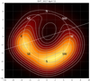 |
Fig. 1. Image of BH M 87* at 1.3 mm wavelength obtained on April 11, 2017, by the EHT (adapted from Fig. 3 in EHT Collaboration 2019a). The grey contour levels correspond to brightness temperature values of (2, 2.5, 3, …, 5.5) × 109 K. The white dashed lines indicate a photon ring of 42 μas in diameter equivalent to ≃11 M, and the position angle of large-scale jet PA = 288° (WNW). The units of the grid are the angular size of the M 87* gravitational radius θg ≃ 3.8 μas. |
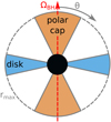 |
Fig. 2. Schematic geometry of the axially symmetric emitting regions in the space of Boyer-Lindquist coordinates (r, θ). The emitting regions are limited to r < rmax = 6 M and θmin < θ, π − θ < θmax. In the case of polar caps (TH1), we adopt θmin = 0 and θmax = 30°. In the case of equatorial disc (TH4), we adopt θmin = 75° and θmax = 90°. |
We first study the effect of location of the emitting regions in the θ space, considering the following four cases: (TH1) θmin = 0 and θmax = 30° (polar caps); (TH2) θmin = 30° and θmax = 45°; (TH3) θmin = 45° and θmax = 75°; and (TH4) θmin = 75° and θmax = 90° (equatorial ring). The results are shown in Fig. 3 for two extreme values of BH spin: a = 0 and a = 0.9. We note that there is only a mild effect of BH spin on the images produced with rmax = 6 M.
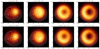 |
Fig. 3. Series of simulated images for source regions limited to the radial coordinate values r ≤ rmax = 6 M and to different values of the polar coordinate (models TH1-4, from left to right) for two values of BH spin. In these cases, the local emitter is assumed to be stationary (βr = 0 = Ω), and the spectral index is α = 0.5. The simulated images are shown with colour shading and grey contours, while the EHT image of M 87* is shown with solid white contours. The contour levels correspond to brightness temperature values of (2.5, 3.5, 4.5, 5.5) × 109 K, both for the simulated images and for the EHT image. The dashed white circle indicates a photon ring of radius 21 μas ≃ 5.5θg (best-fit estimate by EHT). The dashed white line indicates the position angle PAjet = 288° of the large-scale jet. |
In the case of polar caps (TH1), the image is dominated by a single compact hot spot slightly offset from the image centre along the jet direction and coinciding with the middle of the shadow observed by the EHT. This is an image of the front polar cap, while the image of the back polar cap is smeared roughly uniformly along the photon ring. In the case TH2, the image of the front cap becomes extended, but remains centrally peaked. In the case TH3, the image morphology turns into a ring of radius ∼4Rg without a deep shadow on top of a roughly uniform image of the back ring spanning the entire photon ring. Finally, in the case of equatorial ring (TH4), the size of the simulated image becomes consistent with the size of the EHT image, but the brightness distribution along the ring is fairly uniform. The effect of BH spin is that for a = 0 the brightest sector of the ring is the one opposite to the jet direction, while for a = 0.9 the brightest sector is rotated towards the southern side (CW in the case of TH2 and CCW in the case of TH3). Without additional Doppler beaming, there is too much emission from the northern part of the ring.
We now consider the effect of Doppler beaming due to the motion of the emitting plasma. First, in the case of polar caps (TH1), we study the effect of radial infall with fixed coordinate velocity βr. Figure 4 shows that the image of the front cap is strongly suppressed for the radial velocity of βr ≥ 0.4, and we see the image of the back cap magnified into a ring that is slightly brighter on the southern side. This illustrates the basic fact that the kinematics of emitting fluid, which involve mildly relativistic motions, have a very strong effect on the appearance of BH environments.
However, the case of fixed radial velocity, including that of static emitter fluid, is physically unrealistic. Therefore, as the next level of approximation, we consider plunging (βr < 0) time-like geodesic flows that conserve energy E and angular momentum L. We neglect the poloidal four-velocity component uθ = 0. Since the four-velocity components ut and uϕ can be calculated explicitly from E and L, we can then calculate the radial component ur from u2 = −1. We consider the fluid to be constricted to regions where (ur)2 ≥ 0.
Figure 5 presents the case of polar caps (TH1) for the BH spin value of a = 0.5 and fixed asymptotic energy E = 1, showing the effect of moderate angular momentum 0 ≤ L ≤ 0.6. The case of L = 0 is very similar to the case of βr = −0.4; it is a fairly uniform ring with maximum brightness in the SE sector. Introducing non-zero L has a very strong effect. It significantly decreases the brightness along the northern side of the ring, turning it into a crescent already for L = 0.2, although the N–S contrast is still too low, and the second-brightest contour of the crescent is rotated CCW with respect to the observed image. Higher values of L make the image too compact, centred in the S sector.
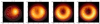 |
Fig. 4. Case of polar caps (TH1) for a = 0.5, showing the effect of Doppler beaming due to radial infall of the emitting fluid with fixed radial velocity βr. See Fig. 3 for further details. |
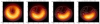 |
Fig. 5. Case of polar caps (TH1) for a = 0.5 with fixed values of conserved energy E and angular momentum L. See Fig. 3 for further details. |
In the case of equatorial rings (TH4), we consider either the plunging geodesic time-like flows with conserved E and L, or quasi-Keplerian circular motions with βr = 0 and angular velocity Ω = Ωcirc, with the rings limited from the inside by the ISCO (innermost stable circular orbit; Bardeen et al. 1972) and from the outside by rmax = 6 M (we only consider prograde discs for a > 0, for which RISCO < 6 M).
Figure 6 compares the images calculated in these two scenarios for two values of BH spin a = 0.5, 0.9. It is notable that these images are very similar to each other, with most of the emission concentrated along the southern side of the photon ring. Our models for plunging flows with fixed E and L provide a very good match with the observed emission in the SSE–WSW sector. On the other hand, emission from the ESE sector is very weak in all cases. It should be stressed that these results are not very sensitive to the choice of E and L values, since the images are very similar for 0.94 ≤ E ≤ 1.3 and for 2 ≤ L ≤ 3.9. Most of these values of E and L allow for flows plunging onto the BH horizon.
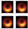 |
Fig. 6. Case of equatorial ring (TH4) for two values of BH spin, with different assumptions on the kinematics of the emitting fluid. Top panels: stable circular orbits with βr = 0 and Keplerian angular velocity Ωcirc(r) within prograde discs limited by rISCO(a) < r < rmax = 6 M. Bottom panels: plunging orbits with conserved energy E and angular momentum L, limited by rh < r < rmax = 6 M. See Fig. 3 for further details. |
3.1. Simulated Event Horizon Telescope observations
Figure 7 shows the results of simulated EHT observations of two representative images. We present the visibility amplitudes Iamp, ij as functions of pair baselines  , and the closure phases ΨC, ijk as functions of triangle baselines
  , and we compare them with the results of EHT observations of M 87 obtained on 2017 April 11 in the high-frequency band.
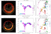 |
Fig. 7. Results of simulated EHT observations of selected model images. Left panels: model images (high resolution in colour scale and EHT resolution with the orange contours) compared with the reference image reconstructed from the actual EHT observations of M 87* obtained on 2017 April 11 (solid white contours). Middle panels: visibility amplitude as a function of telescope pair baseline. The filled circles indicate the actual EHT measurements of M 87*, and the crosses indicate the simulated EHT observations of the model image. The symbol colour indicates the orientation of the telescope pair baseline. Right panels: closure phase as a function of telescope triangle baseline. The symbol colour indicates the telescope triangle indicated by the labels. |
The first simulated image is the case of an equatorial ring with parameters a = 0.5, E = 1, and L = 3. We obtain reasonable agreement between the simulated and observed visibility amplitudes. We note that the normalisation of simulated Iamp values is approximate; it is intended to match the observed visibility for baselines in the range ∼(5 − 7) Gλ, however our model underproduces the total observed flux (Iamp in the limit of zero baseline) by a factor of approximately three. The first minimum of the simulated Iamp is obtained for the E–W baselines: ≃3.6 Gλ, which is slightly longer than for the observed minimum at ≃3.4 Gλ. This minimum is much shallower for the N–S baselines, both for the simulated and real observations3. The second minimum of Iamp at the E–W baselines, ≃8.3 Gλ, is not very deep in the simulated model data.
The closure phases reveal various levels of agreement between the simulated observations of our model and actual measurements of M 87*. Reasonable agreement is found for the SMT-LMT-PV and ALMA-SMT-LMT triangles characterised by intermediate values of triangle baselines, namely ≃(6 − 9) Gλ, as well as for the ALMA-SMT-PV triangle with (10 − 10.5) Gλ. On the other hand, there is a clear discrepancy at the shortest triangle baselines, ≃(3.9 − 4.6) Gλ, where the simulated ΨC,SMT−JCMT/SMA−LMT is consistent with zero, while its observed values span a wide range of intermediate values (20° :140° ). There are also systematic differences between closure phases for the ALMA-LMT-PV (≃140° simulated vs. ≃100° observed), ALMA-JCMT/SMA-LMT (mostly [ − 150° : − 90° ] simulated vs. [ − 90° : − 50° ] observed), and ALMA-SMT-JCMT/SMA (mostly [20° :110° ] simulated vs. [ − 10° :70° ] observed) triangles.
The second simulated image is the case of a polar cap with parameters a = 0.5, E = 1, and L = 0.4. The structure of the visibility amplitude as a function of the pair baseline is very similar to the previous case. The first minimum of Iamp is found at the slightly longer E–W pair baseline of 3.7 Gλ. The simulated closure phases are generally similar to the previous case. Much better agreement is found for the triangles ALMA-SMT-LMT and ALMA-JCMT/SMA-LMT (main group). On the other hand, the simulated values for the triangle ALMA-LMT-PV are shifted to ≃155°, and those for the triangle ALMA-SMT-PV are found at [ − 180° : − 150° ]. For the smallest triangle, namely SMT-JCMT/SMA-LMT, the closure values measured for triangle baselines longer than 5 Gλ are concentrated at [ − 170° : − 130° ].
4. Discussion and conclusions
The EHT image of the BH M 87* could be interpreted either as a single crescent extending from the E to WSW sectors of the photon ring, or as a combination of a short crescent in the SSE–WSW sector and a compact ESE “hotspot”. The GRMHD simulations of geometrically thick accretion onto BHs tend to produce images of crescents that are roughly parallel to the projected jet axis (Dexter et al. 2012; Mościbrodzka et al. 2016; Davelaar et al. 2019). Therefore, these simulations are equally able to explain emission from the SSE–WSW sector as our simplified toy models. This qualitative consistency of results suggests that the ESE emission might require a distinct origin.
In our models of polar caps (TH1), the image of the front polar cap is expected to coincide with the observed position of the BH shadow. Figure 4 demonstrates that radial infall with velocity of βr ∼ 0.4 is able to suppress the image of the front cap, at the same time enhancing the extended image of the back cap. In turn, Fig. 5 shows that the image of the back cap is sensitive to the angular momentum of the plunging flow; with L ≃ 0.4 it is possible to reproduce the required north–south contrast, however emission from the ESE sector is insufficient to explain the EHT observations.
Our models of equatorial rings (TH4) with rmax ≃ 6Rg (Fig. 6) produce crescent images that typically extend from SSE to W position angles, with only weak emission in the ESE sector, almost independently of the adopted kinematic model for the emitter fluid. We considered stable equatorial orbits limited from the inside by ISCO (prograde orbits for a > 0) and plunging flows with conserved energy and angular momentum, and in no case were we able to extend the crescent towards the ESE sector.
The differences between our model images and the reconstructed EHT image of M 87* are reflected in the differences between the closure phases obtained by simulating EHT observations of our images and those actually measured during the EHT observations of M 87*. In our models, we can reproduce the closure phases for certain telescope triangles (e.g. ALMA-SMT-LMT), but never for all of them. In particular, it is difficult to reproduce the highly variable closure phases for the smallest triangle SMT-JCMT/SMA-LMT.
The EHT image of M 87* is insufficient to significantly constrain the value of BH spin because the radius of the photon ring is not sensitive to the spin value (EHT Collaboration 2019d) and the photon ring departs substantially from circularity only for a ≥ 0.95 (Bambi et al. 2019). More stringent constraints come from the requirement for production of sufficiently powerful jets, which essentially eliminates the values |a| < 0.4 (Nokhrina et al. 2019; Nemmen 2019). We find that considering extreme spin values of a = 0 and a = 0.9 does not qualitatively affect the obtained images for rmax = 6Rg. This effect would be much greater for smaller values of rmax (e.g. 3), which would however result in significantly smaller images (for the same value of BH mass). On the other hand, Dokuchaev & Nazarova (2019) argued that the relative orientation of the BH shadow and the brightness centre of the crescent constrains the spin value to a = 0.75 ± 0.15. This latter result was obtained by ray tracing emission from plunging geodesic flows with conserved E and L in an optically thin equatorial disc limited to within the ISCO radius. This latter study suggests that the ESE “hotspot” coincides with the brightest point of the accretion flow, oriented roughly perpendicularly to the BH spin, which is however not consistent with the direction of the large-scale jet.
Our models were calculated under strict assumptions of azimuthal and planar symmetry of the emitting regions. The easiest way to obtain a crescent image of correct orientation is to relax the assumption of azimuthal symmetry, adding an m = 1 mode to the local emissivity. However, from such relaxed models we cannot draw any meaningful constraints on the geometry and velocity fields of the underlying plasma flows. In particular, emission in the ESE sector could be explained by a localised and temporary perturbation in the accretion flow. One possibility for such perturbations are filaments resulting from the interchange instability operating in the magnetically arrested discs (MAD; McKinney et al. 2012). Any such temporary effects should not persist in the subsequent EHT observations. Short-term variations of the EHT images of M 87* are at the level of ≲15% over the time range of 6 days, equivalent to 16Rg/c (EHT Collaboration 2019c, Fig. 33).
It has been suggested that synchrotron self-absorption may have a significant effect on the image of M 87* at the 1.3 mm wavelength if observed eventually in a higher flux state (Kawashima et al. 2019). A potentially more important factor could be anisotropic rest-frame emissivity due to the synchrotron process operating in ordered magnetic fields. While GRMHD simulations are likely to produce realistic distributions of magnetic fields, they typically treat the emitting particles as locally isotropic. On the other hand, it has been argued in the context of relativistic AGN jets that the momenta of energetic electrons could be strongly concentrated along the local magnetic field lines (e.g. Sobacchi & Lyubarsky 2019). Global kinetic numerical simulations or improved subgrid MHD models may be required to incorporate such effects.
The origin of emission observed by the EHT in the ESE sector of the photon ring in M 87* cannot be explained using strictly stationary and axisymmetric models – whether equatorial rings or polar caps – that assume the theoretically expected alignment of the BH spin with the large-scale jet. The most natural solution is to invoke temporary fluctuations of the inner accretion flow magnified along the photon ring (EHT Collaboration 2019d). The ESE “hotspot” can therefore be expected to disappear in the subsequent EHT observations of M 87*.
For the simulated observations reported with inverted baselines (i > j), we reverse the signs of uji = −uij, vji = −vij and Ψji = −Ψij.
More strictly, we define the triangle chirality as sijk = sign[(u, v)ij ∧ (u, v)jk]. The triangle (1,2,4) or ALMA-SMT-LMT changes its chirality from s124 = +1 to s124 = −1 at  . To avoid flipping the sign of ΨC, 124, we adopted a fixed value of s124 = +1.
This is entirely consistent with the results presented by the EHT Collaboration in Fig. 1 of EHT Collaboration (2019b), where the E–W baselines are shown in blue and the N–S baselines are shown in red.
Acknowledgments
We thank the anonymous reviewer for helpful suggestions. We acknowledge discussions with Bartosz Bełdycki, Benoît Cerutti, Christian Fromm, Jean-Pierre Lasota and Maciej Wielgus. We have used the eht-imaging software (Chael et al. 2016, 2018) obtained from https://github.com/achael/eht-imaging, and the EHT Science Release 1 (SR1) dataset (EHT Collaboration 2019e) obtained from https://eventhorizontelescope.org/for-astronomers/data. This work was partially supported by the Polish National Science Centre grants 2015/18/E/ST9/00580 and 2015/17/B/ST9/03422.
References
- Abramowski, A., Acero, F., Aharonian, F., et al. 2012, ApJ, 746, 151 [NASA ADS] [CrossRef] [Google Scholar]
- Aharonian, F., Akhperjanian, A. G., Bazer-Bachi, A. R., et al. 2006, Science, 314, 1424 [NASA ADS] [CrossRef] [PubMed] [Google Scholar]
- Bambi, C., Freese, K., Vagnozzi, S., et al. 2019, Phys. Rev. D, 100, 044057 [NASA ADS] [CrossRef] [Google Scholar]
- Bardeen, J. M., Press, W. H., & Teukolsky, S. A. 1972, ApJ, 178, 347 [NASA ADS] [CrossRef] [Google Scholar]
- Blandford, R. D., & Znajek, R. L. 1977, MNRAS, 179, 433 [NASA ADS] [CrossRef] [Google Scholar]
- Broderick, A. E., & Tchekhovskoy, A. 2015, ApJ, 809, 97 [NASA ADS] [CrossRef] [Google Scholar]
- Chael, A. A., Johnson, M. D., Narayan, R., et al. 2016, ApJ, 829, 11 [NASA ADS] [CrossRef] [Google Scholar]
- Chael, A. A., Johnson, M. D., Bouman, K. L., et al. 2018, ApJ, 857, 23 [Google Scholar]
- Davelaar, J., Olivares, H., Porth, O., et al. 2019, A&A, 632, A2 [NASA ADS] [CrossRef] [EDP Sciences] [Google Scholar]
- Dexter, J., McKinney, J. C., & Agol, E. 2012, MNRAS, 421, 1517 [NASA ADS] [CrossRef] [Google Scholar]
- Dokuchaev, V. I., & Nazarova, N. O. 2019, Universe, 5, 183 [NASA ADS] [CrossRef] [Google Scholar]
- Event Horizon Telescope Collaboration (Akiyama, K., et al.) 2019a, ApJ, 875, L1 [NASA ADS] [CrossRef] [Google Scholar]
- Event Horizon Telescope Collaboration (Akiyama, K., et al.) 2019b, ApJ, 875, L6 [Google Scholar]
- Event Horizon Telescope Collaboration (Akiyama, K., et al.) 2019c, ApJ, 875, L4 [NASA ADS] [CrossRef] [Google Scholar]
- Event Horizon Telescope Collaboration (Akiyama, K., et al.) 2019d, ApJ, 875, L5 [NASA ADS] [CrossRef] [Google Scholar]
- Event Horizon Telescope Collaboration 2019e, First M87 EHT Results: Calibrated Data, CyVerse Data Commons https://doi.org/10.25739/g85n-f134 [Google Scholar]
- Hada, K., Kino, M., Doi, A., et al. 2016, ApJ, 817, 131 [NASA ADS] [CrossRef] [Google Scholar]
- Katsoulakos, G., & Rieger, F. M. 2018, ApJ, 852, 112 [NASA ADS] [CrossRef] [Google Scholar]
- Kawashima, T., Kino, M., & Akiyama, K. 2019, ApJ, 878, 27 [NASA ADS] [CrossRef] [Google Scholar]
- Kim, J.-Y., Krichbaum, T. P., Lu, R.-S., et al. 2018, A&A, 616, A188 [NASA ADS] [CrossRef] [EDP Sciences] [Google Scholar]
- Levinson, A., & Rieger, F. 2011, ApJ, 730, 123 [NASA ADS] [CrossRef] [Google Scholar]
- Martocchia, A., & Matt, G. 1996, MNRAS, 282, L53 [NASA ADS] [CrossRef] [Google Scholar]
- McKinney, J. C., Tchekhovskoy, A., & Blandford, R. D. 2012, MNRAS, 423, 3083 [NASA ADS] [CrossRef] [Google Scholar]
- McKinney, J. C., Tchekhovskoy, A., & Blandford, R. D. 2013, Science, 339, 49 [NASA ADS] [CrossRef] [PubMed] [Google Scholar]
- Mertens, F., Lobanov, A. P., Walker, R. C., & Hardee, P. E. 2016, A&A, 595, A54 [NASA ADS] [CrossRef] [EDP Sciences] [Google Scholar]
- Miniutti, G., & Fabian, A. C. 2004, MNRAS, 349, 1435 [NASA ADS] [CrossRef] [Google Scholar]
- Mościbrodzka, M., & Gammie, C. F. 2018, MNRAS, 475, 43 [NASA ADS] [CrossRef] [Google Scholar]
- Mościbrodzka, M., Falcke, H., & Shiokawa, H. 2016, A&A, 586, A38 [NASA ADS] [CrossRef] [EDP Sciences] [Google Scholar]
- Nemmen, R. 2019, ApJ, 880, L26 [NASA ADS] [CrossRef] [Google Scholar]
- Nokhrina, E. E., Gurvits, L. I., Beskin, V. S., et al. 2019, MNRAS, 489, 1197 [NASA ADS] [CrossRef] [Google Scholar]
- Parfrey, K., Philippov, A., & Cerutti, B. 2019, Phys. Rev. Lett., 122, 035101 [NASA ADS] [CrossRef] [Google Scholar]
- Sikora, M. 1979, PhD Thesis, Nicolaus Copernicus Astronomical Center, Polish Academy of Sciences [Google Scholar]
- Sobacchi, E., & Lyubarsky, Y. E. 2019, MNRAS, 484, 1192 [NASA ADS] [CrossRef] [Google Scholar]
- Walker, R. C., Hardee, P. E., Davies, F. B., Ly, C., & Junor, W. 2018, ApJ, 855, 128 [NASA ADS] [CrossRef] [Google Scholar]
All Figures
|
Fig. 1. Image of BH M 87* at 1.3 mm wavelength obtained on April 11, 2017, by the EHT (adapted from Fig. 3 in EHT Collaboration 2019a). The grey contour levels correspond to brightness temperature values of (2, 2.5, 3, …, 5.5) × 109 K. The white dashed lines indicate a photon ring of 42 μas in diameter equivalent to ≃11 M, and the position angle of large-scale jet PA = 288° (WNW). The units of the grid are the angular size of the M 87* gravitational radius θg ≃ 3.8 μas. |
| In the text | |
|
Fig. 2. Schematic geometry of the axially symmetric emitting regions in the space of Boyer-Lindquist coordinates (r, θ). The emitting regions are limited to r < rmax = 6 M and θmin < θ, π − θ < θmax. In the case of polar caps (TH1), we adopt θmin = 0 and θmax = 30°. In the case of equatorial disc (TH4), we adopt θmin = 75° and θmax = 90°. |
| In the text | |
|
Fig. 3. Series of simulated images for source regions limited to the radial coordinate values r ≤ rmax = 6 M and to different values of the polar coordinate (models TH1-4, from left to right) for two values of BH spin. In these cases, the local emitter is assumed to be stationary (βr = 0 = Ω), and the spectral index is α = 0.5. The simulated images are shown with colour shading and grey contours, while the EHT image of M 87* is shown with solid white contours. The contour levels correspond to brightness temperature values of (2.5, 3.5, 4.5, 5.5) × 109 K, both for the simulated images and for the EHT image. The dashed white circle indicates a photon ring of radius 21 μas ≃ 5.5θg (best-fit estimate by EHT). The dashed white line indicates the position angle PAjet = 288° of the large-scale jet. |
| In the text | |
|
Fig. 4. Case of polar caps (TH1) for a = 0.5, showing the effect of Doppler beaming due to radial infall of the emitting fluid with fixed radial velocity βr. See Fig. 3 for further details. |
| In the text | |
|
Fig. 5. Case of polar caps (TH1) for a = 0.5 with fixed values of conserved energy E and angular momentum L. See Fig. 3 for further details. |
| In the text | |
|
Fig. 6. Case of equatorial ring (TH4) for two values of BH spin, with different assumptions on the kinematics of the emitting fluid. Top panels: stable circular orbits with βr = 0 and Keplerian angular velocity Ωcirc(r) within prograde discs limited by rISCO(a) < r < rmax = 6 M. Bottom panels: plunging orbits with conserved energy E and angular momentum L, limited by rh < r < rmax = 6 M. See Fig. 3 for further details. |
| In the text | |
|
Fig. 7. Results of simulated EHT observations of selected model images. Left panels: model images (high resolution in colour scale and EHT resolution with the orange contours) compared with the reference image reconstructed from the actual EHT observations of M 87* obtained on 2017 April 11 (solid white contours). Middle panels: visibility amplitude as a function of telescope pair baseline. The filled circles indicate the actual EHT measurements of M 87*, and the crosses indicate the simulated EHT observations of the model image. The symbol colour indicates the orientation of the telescope pair baseline. Right panels: closure phase as a function of telescope triangle baseline. The symbol colour indicates the telescope triangle indicated by the labels. |
| In the text | |
Current usage metrics show cumulative count of Article Views (full-text article views including HTML views, PDF and ePub downloads, according to the available data) and Abstracts Views on Vision4Press platform.
Data correspond to usage on the plateform after 2015. The current usage metrics is available 48-96 hours after online publication and is updated daily on week days.
Initial download of the metrics may take a while.