| Issue |
A&A
Volume 634, February 2020
|
|
|---|---|---|
| Article Number | A23 | |
| Number of page(s) | 19 | |
| Section | Planets and planetary systems | |
| DOI | https://doi.org/10.1051/0004-6361/201936281 | |
| Published online | 31 January 2020 | |
Dust in brown dwarfs and extra-solar planets
VII. Cloud formation in diffusive atmospheres
1
Centre for Exoplanet Science, University of St Andrews,
St Andrews, UK
e-mail: This email address is being protected from spambots. You need JavaScript enabled to view it.
2
SUPA, School of Physics & Astronomy, University of St Andrews,
St Andrews,
KY16 9SS, UK
3
SRON Netherlands Institute for Space Research,
Sorbonnelaan 2,
3584 CA
Utrecht, The Netherlands
4
SUPA, School of Physics and Astronomy, University of Edinburgh,
Edinburgh,
EH9 3JZ,
UK
Received:
10
July
2019
Accepted:
9
November
2019
Abstract
The precipitation of cloud particles in brown dwarf and exoplanet atmospheres establishes an ongoing downward flux of condensable elements. To understand the efficiency of cloud formation, it is therefore crucial to identify and quantify the replenishment mechanism that is able to compensate for these local losses of condensable elements in the upper atmosphere, and to keep the extrasolar weather cycle running. In this paper, we introduce a new cloud formation model by combining the cloud particle moment method we described previously with a diffusive mixing approach, taking into account turbulent mixing and gas-kinetic diffusion for both gas and cloud particles. The equations are of diffusion-reaction type and are solved time-dependently for a prescribed 1D atmospheric structure, until the model has relaxed toward a time-independent solution. In comparison to our previous models, the new hot-Jupiter model results (Teff ≈ 2000 K, log g = 3) show fewer but larger cloud particles that are more concentrated towards the cloud base. The abundances of condensable elements in the gas phase are featured by a steep decline above the cloud base, followed by a shallower, monotonous decrease towards a plateau, the level of which depends on temperature. The chemical composition of the cloud particles also differs significantly from our previous models. Through the condensation of specific condensates such as Mg2SiO4[s] in deeper layers, certain elements, such as Mg, are almost entirely removed early from the gas phase. This leads to unusual (and non-solar) element ratios in higher atmospheric layers, which then favours the formation of SiO[s] and SiO2[s], for example, rather than MgSiO3[s]. These condensates are not expected in phase-equilibrium models that start from solar abundances. Above the main silicate cloud layer, which is enriched with iron and metal oxides, we find a second cloud layer made of Na2S[s] particles in cooler models (Teff ⪅ 1400 K).
Key words: diffusion / brown dwarfs / planets and satellites: atmospheres / planets and satellites: composition / astrochemistry
© ESO 2020
1 Introduction
More than 4000 extrasolar planets have been confirmed to date, but only a handful of them can be studied in detail (see e.g. Nikolov et al. 2016; Huitson et al. 2017; Birkby et al. 2017; Arcangeli et al. 2018). Indirect observations, for instance transmission spectroscopy, have demonstrated the presence of clouds (Sing et al. 2016; Nikolov et al. 2016; Pino et al. 2018; Gibson et al. 2017; Kirk et al. 2018; Tregloan-Reed et al. 2018). Far easier targets for atmosphere studies are brown dwarfs, which are very similar to planets with respect to their physical parameters and atmospheric processes. The coolest brown dwarfs (Y dwarfs) reach effective temperatures as low as 250 K (Leggett et al. 2017; Luhman 2014). The observation of brown dwarfs allows us to identify the vertical cloud structures (Apai et al. 2013; Buenzli et al. 2015; Yang et al. 2016; Helling & Casewell 2014). To date, between 1500 and 2000 brown dwarfs are known (depending on whether late-M dwarfs and/or early-L dwarfs are included; Gagné et al. 2015; Best et al. 2018) and are relatively well studied compared to the ~4000 extrasolar planets, for which the era of spectral analysis has only just begun.
Cloud formation has a profound impact on the remaining gas-phase abundances and radiative transfer effects, but cloud particles will also affect the ionisation state of the atmosphere, which is well known for Solar System objects (Helling et al. 2016a,b). Efforts are therefore ongoing to construct physical models describing the formation of clouds in exoplanet and brown dwarf atmospheres. Detailed models like this are necessary tools to provide the context for observations and to uncover processes that are not directly accessible by observations. Part of this effort is the consistent coupling of cloud formation with 1D atmosphere models with radiative transfer and convection (Tsuji et al. 1996; Ackerman & Marley 2001; Tsuji 2002; Witte et al. 2009; Allard et al. 2012; Juncher et al. 2017; also Helling et al. 2008a), but also in 3D in order to study the time-dependent climate of extrasolar planets (Lee et al. 2016; Lines et al. 2018) and to understand observational implications beyond 1D (Lee et al. 2017; Lines et al. 2018).
As our understanding of cloud formation progresses (e.g. Lee et al. 2015b; Krasnokutski et al. 2017; Hörst et al. 2019), including its implication for habitability (Narita et al. 2015), we start to refine our approaches. One long-standing discussion is how to model the element replenishment in 1D cloud-forming atmospheres, because without replenishment, a quasi-static atmosphere must be cloud free (Appendix A in Woitke & Helling 2004). Parmentier et al. (2013) used passive tracers to study the atmospheric mixing in 3D (shallow water approximation) simulations for irradiated dynamic but convectively stable atmospheres of (gas giant) planets. They observed that cloud particles are distributed throughout the whole atmosphere.
Parmentier et al. (2013) pointed out that in their relaxed hydrodynamical models, the upward transport by mixing statistically balances the downward transport due to particle settling. The mixing does not require convection in particular, but any large-scale vertical motions in the stably stratified atmosphere can provide such mixing. These flow patterns need to be revealed by global circulation models, for example driven by the day-night heating contrast. This assessment confirms our conclusion that the upward transport of condensable elements through the atmosphere by mixing is indeed the key for understanding cloud formation. However, challenges arise from the choice of the inner boundary condition (Carone et al. 2019), chemical gradients (Tremblin et al. 2019), and the need to include cloud particle feedback in order to test mixing parametrisations. A particular interesting case will be the ultra-hot Jupiters, where day and night sides can be expected to have very distinct (vertical) mixing patterns and scales. In this paper, we consider self-luminous gas giant planets, for which the irradiation from their host stars is negligible, such as young gas giant planets and brown dwarfs. Brown dwarf atmospheres are by now understood to be rather similar to gas giant planets, in particular atmospheres from low-gravity brown dwarfs and young gas giants (Charnay et al. 2018).
Moses et al. (2000) pointed out that large-scale mixing helps to homogenise a gravitationally stratified atmospheres consisting of different types of molecules. However, this only prevails up to a certain altitude above which gas-kinetic diffusion starts to dominate mixing (Zahnle et al. 2016). Different approaches have been chosen to represent this vertical mixing in 1D atmosphere models (Ackerman & Marley 2001; Woitke & Helling 2004; Helling et al. 2008a; Allard 2014; Juncher et al. 2017) and in 3D models (Lee et al. 2015a; Lines et al. 2018) by measuring vertical velocity fluctuations and deriving mixing parametrisations from 2D or 3D radiation-hydrodynamics simulations (Ludwig et al. 2002; Freytag et al. 2010; Parmentier et al. 2013; Zhang & Showman 2018).
Cloud formation modelling also becomes an increasingly important part of exoplanet and brown dwarf retrieval approaches for which, however, computational speed is an essential limitation. As part of the ARCiS1 retrieval platform, Ormel & Min (2019) presented a new forward-model that consistently solves diffusive mixing and cloud particle growth for exoplanet atmospheres.
In this paper, we present a new theoretical approach that consistently combines cloud formation modelling with diffusive transport for element replenishment. After presenting the main formula body of our model in Sects. 2.1–2.3, we summarise our ansatz for handling the diffusion coefficient in Sect. 2.4, before we present our main results in Sects. 4 and 5. We conclude in Sect. 6. An overview of quantifying diffusion coefficients in the literature is provided in Appendix D.
2 Cloud formation with diffusive transport of gas and cloud particles
Cloud formation involves at least seed particle formation (nucleation), surface growth and evaporation, element depletion, gravitational settling, and element replenishment. During their descent through the atmosphere, cloud particles may change phase, or more general, chemical composition, and may collide with each other, which leads to further growth. These cloud formation processes have been described previously (Woitke & Helling 2003; Helling & Woitke 2006; Helling & Fomins 2013), and different cloud formation models have been compared by Helling et al. (2008a) with an update by Charnay et al. (2018). We therefore only provide a short summary here. A recent review can be found in Helling (2019).
Clouds are made of particles (aerosols, droplets, and solid particles). The formation of these particles requires condensation seeds, which are produced, for the case of the Earth atmosphere, by volcano eruptions, ocean sprays, and wild fires. In absence of these crucial processes, which all require the existence of a solid planet surface, cloud formation needs to start with the formation of seed particles through chemical reactions in the gas phase, involving the formation of molecular clusters. The formation of seed particles requires a highly supersaturated gas. Once such seed particles become available, many materials are already thermally stable and can simultaneously condense onto these surfaces. Nucleation and growth reduce the local element abundances and have a strong feedback on the local composition of the atmospheric gas. As macroscopic cloud particles form, they display a spectrum of sizes as well as a mixture of condensed materials. The local particle size distribution and the material mixture change as the cloud particles move through the atmosphere (hence, encounter different thermodynamic conditions), for example by gravitational settling (rain). Particle–particle collision will continue to shape the size distribution function. Cloud particles may break up into smaller units (shattering) or stick together to form even larger units (coagulation). Cloud particles may also be transported upward and downward by macroscopic mixing processes. Particle–particle processes are not part of our present model, which focuses on the formation of cloud particles and their feedback on the local chemistry through element depletion or enrichment. We note that the surface growth does shut off the nucleation process due to efficient element depletion (Lee et al. 2015b) such that a simultaneous treatment of nucleation and growth is required in order to calculate the number of cloud particles that form in the first place.
2.1 Cloud formation as a reaction-diffusion system
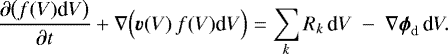
As introduced in Woitke & Helling (2003), we consider the evolution of the size distribution function f(V) [cm−6] of cloud particles in the particle volume interval V... V + dV as affected by advection, settling, surface reactions, and (new) by diffusion according to the following master equation:
 (1)
(1)
Rk are the various gain and loss rates due to surface chemical reactions, which lead to growth and evaporation of the particles (see Eqs. (59)–(62) for large Knudsen numbers, and Eqs. (68)–(71) for small Knudsen numbers in Woitke & Helling 2003). A list of symbols with physical meaning and units is provided in Table 1. The volume of the particles V is chosen as size variable to formulate the material deposit by surface reactions in the most straightforward way. The last term in Eq. (1) accounts for the additional gains and losses due to diffusive mixing. The cloud particle velocity v(V) is assumed to be given by the hydrodynamical gas velocity vgas plus a vertical equilibrium drift velocity 
 (2)
(2)
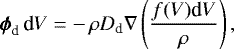
When we apply Fick’s first law (see e.g. Bringuier 2013), the diffusive flux ϕd of the cloud particles in volume interval V... V + dV (ϕd d V has units [cm−2 s−1]) is given by the concentration gradient of these particles,
 (3)
(3)
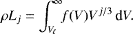
where Dd [cm2 s−1] is the diffusion coefficient for these cloud particles and ρ [g∕cm3] is the gas density. We introduce moments of the cloud particle size distribution as
 (4)
(4)
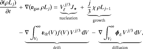
Multiplying Eq. (1) with Vj∕3 and integrating over volume, we obtain the following system of moment equations for large Knudsen numbers (see details in Woitke & Helling 2003):
 (5)
(5)
where J⋆ [s−1 cm−3] is the nucleation rate and χ [cm s−1] the net growth velocity. For large Knudsen numbers and subsonic velocities (Epstein regime), the equilibrium drift velocity, also called final fall speed, is given by Schaaf (1963),
 (6)
(6)
where a is the particle radius, ρd is the cloud particle material density,  is the unit vector pointing away from the centre of gravity, and g is the gravitational acceleration.
  is an abbreviation, T is the temperature, k is the Boltzmann constant, and
  is the mean molecular weight of the gas particles.
Using Eq. (6) with  and assuming that the particle diffusion coefficient Dd is independent of size, we can carry out the integrations in Eq. (5). The final result is
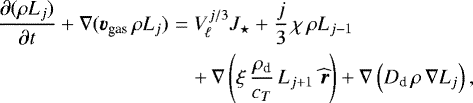 (7)
(7)
with abbreviation
 (8)
(8)
A size-dependent diffusion coefficient, Dd(V), would lead to an open set of moment equations. This has been discussed by Helling & Fomins (2013).
2.2 Generalisation to mixed materials
We assume that all cloud particles are perfect spheres with a well-mixed material composition that is independent of size, but depends on time and location in the atmosphere (Helling & Woitke 2006; Helling et al. 2008c). Using the index s = 1 ... S to distinguish between the different solid materials, for example Al2 O3[s], TiO2 [s], Mg2 SiO4[s] and Fe[s], we write
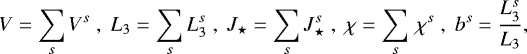 (9)
(9)
where bs is the volume fraction of material s in the cloud particles2. The mean cloud particle material density is given by ρd = ∑sbsρs, where ρs is the mass density of a pure material s. Most materials will not nucleate themselves ( ), but will use alien nuclei to grow on. Using this approximation, we can split the third-moment equation into a set of third-moment equations for single materials as follows:
 (10)
(10)
When we sum Eq. (10) for all solids s, we again obtain Eq. (7) for j = 3. The different materials grow at different speeds that depend on the amount of available atoms and molecules in the gas phase and on the supersaturation ratio. Islands of some materials may grow, whereas others are thermally unstable and shrink. This behaviour is obtained by summing the contributions of all surface reactions r = 1... R (for examples, see Table 1 in Helling et al. 2008c)
 (11)
(11)
where ![Mathematical equation: $V_0^s\rm\,[cm^3]$](/articles/aa/full_html/2020/02/aa36281-19/aa36281-19-eq18.png) is the volume of one unit of material s in the solid state and
is the volume of one unit of material s in the solid state and ![Mathematical equation: $c_r^s\rm\,[cm^{-2}\,s^{-1}]$](/articles/aa/full_html/2020/02/aa36281-19/aa36281-19-eq19.png) is the effective surface reaction rate,
is the effective surface reaction rate,
![Mathematical equation: \begin{equation*} c_r^s = \sqrt[3]{36\pi}\; \frac{\nu_r^s\,n_r^{\textrm{key}}\textrm{v}_r^{\textrm{rel}}\,\alpha_r}{\nu_r^{\textrm{key}}} \left(1-\frac{1}{S_{\!r}}\right) \times \left\{\begin{array}{@{}ll} 1 & \mbox{if\ \ } S_{\!r}\geq 1 \\ b^s & \mbox{if\ \ } S_{\!r}<1 \end{array}\right.\!\!,\end{equation*}](/articles/aa/full_html/2020/02/aa36281-19/aa36281-19-eq20.png) (12)
(12)
where  is the particle density [cm−3] of the key species of surface reaction r, αr is the sticking probability,
  is its stoichiometric factor in that reaction,
  is its thermal relative velocity, and mkey is its mass. These growth rates are derived from a simple hit-and-stick model, where we commonly assume αr = 1. The impact of the limited number of known αr ≠ 1 has been studied by Helling & Woitke (2006). Sr is the reaction supersaturation ratio as introduced in Appendix B of Helling & Woitke (2006). For example, in the reaction
![Mathematical equation: \begin{equation*} \rm 2\,CaH ~+~ 2\,Ti ~+~ 6\,H_2O ~\longleftrightarrow~ 2\,CaTiO_3[s] ~+~ 7\,H_2 \end{equation*}](/articles/aa/full_html/2020/02/aa36281-19/aa36281-19-eq24.png) (13)
(13)
the key species is either CaH or Ti, depending on which species is less abundant.  in either case, s = CaTiO3[s] is the solid species, and
  units of CaTiO3[s] are produced by one reaction.
We note that Eq. (12) differs slightly from our previous definition (Eq. 4 in Helling et al. 2008c). The new growth/evaporation rates now always change sign at Sr = 1 as they should, independent of the value of bs. When supersaturated (Sr > 1), we assume that the total surface of the particles acts as a funnel to collect the impinging molecules from the gas phase, followed by fast hopping to find a place on a matching island of kind s (see Fig. 1 in Helling & Woitke 2006). For under-saturation (Sr < 1), however, we assume that the molecules triggering the evaporation processes must hit one of the islands of the matching kind, the probability of which is bs.
Variable definitions and units.
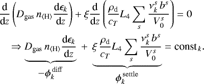
2.3 Element conservation with diffusive replenishment
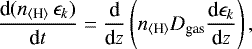
An integral part of our cloud formation model is the element conservation. We must identify a replenishment mechanism that is able to compensate for the losses of elements due to cloud particle formation and settling in the upper atmosphere. In this paper, we include diffusion of gas particles along their concentration gradients. As cloud particles form, they consume certain elements in the upper atmosphere, creating a negative element abundance gradient. Thus, gas particles containing these elements will ascent diffusively in the atmosphere. Analogously to the formulation of the master equation for the dust particles, we formulate the element conservation as diffusion-reaction system,
 (14)
(14)
where ɛk is the abundance of element k with respect to hydrogen. The chemical reactions leading to nucleation and growth appear as negative source terms here because they consume elements. We chose n⟨H⟩ as density variable in Eq. (14), the total hydrogen nuclei particle density, which is proportional to ρ in hydrogen-dominated atmospheres. n⟨H⟩ɛk is the total number density [cm−3] of nuclei of element k in any chemical form.  is the stoichiometric factor of element k in solid s, for example
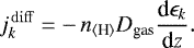
 ![Mathematical equation: $\nu_{\textrm{Ti}}^{\textrm{TiO2[s]}}=1$](/articles/aa/full_html/2020/02/aa36281-19/aa36281-19-eq29.png) , and Dgas [cm2 s−1 ] is the gas diffusion coefficient. For simplicity, we assumed that all molecules are transported by the same diffusion coefficient, which is valid within a factor 2 or 3 for gas-kinetic diffusion (sometimes called the binary diffusion coefficient, see Eq. (16) and Appendix D), and is entirely justified when eddy diffusion dominates. The involved diffusive gas element flux
, and Dgas [cm2 s−1 ] is the gas diffusion coefficient. For simplicity, we assumed that all molecules are transported by the same diffusion coefficient, which is valid within a factor 2 or 3 for gas-kinetic diffusion (sometimes called the binary diffusion coefficient, see Eq. (16) and Appendix D), and is entirely justified when eddy diffusion dominates. The involved diffusive gas element flux  [cm−2s−1] is given by
 (15)
(15)
2.4 Gas diffusion coefficient
The diffusion coefficients provide the kinetic information for calculating the transport rates from concentration gradients (e.g. Lamb & Verlinde 2011). In general, gas and cloud particles diffuse with different efficiencies because of their different inertia and collisional cross-sections with the surrounding gas.
The determination of the gas diffusion coefficient Dgas is of crucial importance for our model. We included gas-kinetic diffusion and large-scale turbulent (eddy) diffusion as mixing processes. The gas-kinetic diffusion coefficient is given by
 (16)
(16)
where ℓ = 1∕(σ n) is the mean free path, n is the total gas particle density, and σ ≈ 2.1 × 10⁻¹⁵ cm2 is a typical cross-section for collisions between the molecules under consideration with H2. The thermal velocity is defined as  , where mred is the reduced mass for collisions between the molecule and H2 (Woitke & Helling 2003). This gas-kinetic diffusion ∝ 1∕n is negligible in the lower high-density layers of brown dwarf and planetary atmospheres, where instead mixing by large-scale turbulent orconvective motions is the dominant mixing process (Ackerman & Marley 2001; Ludwig et al. 2002; Woitke & Helling 2004; Allard et al. 2012; Parmentier et al. 2013; Lee et al. 2015a). The large-scale (turbulent, convective, or eddy) gas diffusion coefficient is given by
 (17)
(17)
where ⟨vz⟩ is the root-mean-square average of the fluctuating part of the vertical velocity in the atmosphere,considering averages over sufficiently large volumes and/or long integration times, L is the mixing length, and Hp is the local pressure scale height. α is a dimensionless parameter of the order of one. We used α = 1 in this work,but α can be fine-tuned to describe the actual mixing scales as revealed by detailed hydrodynamic modelling. Inside the convective part of the atmosphere ⟨vz⟩≈vconv was assumed, where vconv is the convective velocity, which is an integral part of stellar atmosphere models, derived from mixing length theory in 1D models. Above the convective atmosphere, where the Schwarzschild criterion for convection is false, ⟨vz ⟩ decreases rapidly with increasing z, but never quite reaches zero due to convective overshoot (see e.g. Brandenburg 2016). We applied a power law in log p to approximate this behaviour,
 (18)
(18)
with a free parameter β′≈ 0.0... 2.2 (Ludwig et al. 2002). The total gas diffusion coefficient is then
 (19)
(19)
At high altitudes, the gas density n is low and hence Dmicro is large, whereas Dmix is small when β′ > 0. Therefore, at some pressure level in the atmosphere, the gas-kinetic diffusion will start to dominate. Figure 1 shows a typical structure as assumed in our models. The minimum of Dgas around 10−3 mbar correspondsto the cross-over point (called the homopause), upward of which Dmicro dominates and the atmospheres is not well mixed. Moses et al. (2000) drew similar conclusions concerning Saturn’s atmosphere. The maximum of Dgas around pconv = 0.2 bar results from the start of the convective layer, within which both ⟨vz⟩ and Dgas are approximately constant. Appendix D summarises some of the formulas currently applied in the literature for the gas diffusion coefficient.
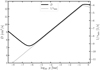 |
Fig. 1 Gas diffusion coefficient Dgas (Eq. (19)) in the new DIFFUDRIFT model for a brown dwarf atmosphere model with Teff = 1800 K, log g =3 [cm s−2] and solar abundances. The grey line shows the inverse mixing timescale τmix as assumed in the previous DRIFT model. τmix is calculated according to Eq. (9) in Woitke & Helling (2004). Both quantities are computed for β = β′ = 1, and both y-axes show exactly eight orders of magnitude. |
2.5 Cloud particle diffusion coefficient
The diffusion of solid particles due to turbulent gas fluctuations was studied, in consideration of protoplanetary discs, by Dubrulle et al. (1995), Schräpler & Henning (2004), Youdin & Lithwick (2007), and Riols & Lesur (2018). All works applied mean field theory (also called Reynolds decomposition ansatz), where the densities and velocities of both the particles and the gas are decomposed into a mean component (that depends only on z) and a small fluctuating part.
The response of the solid particles to the turbulent gas variations is then determined by comparing two timescales. The stopping or frictional coupling timescale is given by
 (20)
(20)
where a is the particle radius. Equation (20) follows from a general relaxation ansatz  , see Eq. (21) in Woitke & Helling (2003), for the special case of large Knudsen numbers in a subsonic flow (the so-called Epstein regime), which we assume is valid here.
The second timescale is the eddy turnover or turbulence correlation timescale τeddy(l) in consideration of a spectrum of different turbulent modes associated with different wave-numbers k or different spatial eddy sizes l. In a Kolmogorov type of power spectrum P(k) ∝ k−5∕3, any given cloud particle of size a tends to co-move with all sufficiently large and slow turbulent eddies, whereas its inertia prevents it from following the short-term, small turbulence modes.
In order to arrive at an effective particle diffusion coefficient, the advective effect of all individual turbulent eddies has to be averaged and thereby transformed into a collective diffusive effect. This procedure is carried out with different procedures and approximations. The result of Schräpler & Henning (2004, see their Eq. (27)) reads
 (21)
(21)
where Dd is the size-dependent cloud particle diffusion coefficient and St is the Stokes number of the particle in consideration of the largest eddy size L. The eddy turnover timescale of the largest turbulence mode is given by
 (22)
(22)
Both the size of the largest eddy L and the average of the fluctuating part of the vertical velocity ⟨vz⟩ are assumedto be identical to the mixing length and velocity appearing in Eq. (17). Combining the above equations, we find
 (23)
(23)
The impact of the size dependence of Dd on the cloudparticle moments was explored by Helling & Fomins (2013), who showed that this leads to an open set of moment equations, which seems impractical for an actual solution. In the frame of this work, we therefore only explore the two limiting cases of very large and very small Stokes numbers throughout the atmosphere. For small particles with St ≪ 1, we have Dd → Dmix and for huge particles St →∞, we have Dd → 0.
 (24)
(24)
Our results show that both approximations lead to rather similar cloud structures in the models explored so far, that is, the inclusion of turbulent cloud particle motions does not seem to be a critical ingredient to our present model. However, in preliminary models for hot Jupiters, where Dmix(z) is flatter or even increases with height, this might be different.
3 Static plane-parallel atmosphere
Before we proceed with the numerical solution of the full time-dependent model of cloud formation in diffusive media, we first discuss the 1D static case in order to better understand the expected results from these equations. When we consider the plane-parallel (∇→d∕dz), static (vgas = 0), and stationary case (∂∕∂t = 0), our Eqs. (7), (10) and (14) simplify to

3.1 Total element fluxes
In the hydrostatic stationary case, the total vertical flux of elements (due to vertical settling of cloud particles and diffusive transport) must be zero everywhere in the atmosphere and for each element. This conclusion can be derived formally by summing Eq. (27) and ∑s (Eq. (26))  , using
  . The chemical source terms (nucleation and growth terms) cancel out exactly, and in case Dd = 0, we find
 (28)
(28)
 [cm−2 s1 ] is the upward element flux by diffusion in the gas phase and
  is the downward flux of elements contained in the settling cloud particles at this point. Equation (28) would still allow for solutions with constant (i.e. time-independent and height-independent) total element fluxes throughout the atmosphere, but this would require matching feeding and removing rates at the bottom and the base of the atmosphere, which does not seem to be physically plausible.
3.2 Equlibrium between gas diffusion and particle settling
From Eq. (28), assuming constk = 0, we find
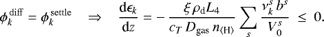 (29)
(29)
The element abundance gradients in a cloudy, static (vgas = 0), and stationary (∂∕∂t = 0) atmosphere must be negative. The downward transport of elements through the precipitation of cloud particles must be balanced by an upward-directed diffusive flux of elements in the gas phase, which requires a negative concentration gradient in the gas phase. This conclusion is correct whenever cloud particles are present (L4 > 0) and gravity is active (ξ > 0), otherwise, the gas element abundances are constant. The abundance gradients of different elements are proportional to the element composition of the settling cloud particles at this point. The abundances of all elements k involved in cloud formation must decrease monotonically toward the top of the atmosphere.
4 Numerical solution of the time-dependent cloud formation problem
Equations (25)-(27) form a system of (3 + S + K) coupled second-order differential equations, which can be transformed into a system of 2 × (3 + S + K) first-order ordinary differential equations (ODEs). Unfortunately, we have not been able to solve this ODE system directly. The boundary conditions are partly given at the lower and partly at the upper boundary of the model, see Sect. 4.4. The integration direction must be downward in order to model the nucleation of new cloud particles. Hence, we tried a shooting method where ɛk (zmax) was varied at the top of the atmosphere until ɛk(zmin) was met, that is, the given values in the deep atmosphere. We found it impossible to proceed this way. A tiny change of ɛk (zmax) in the 12th digit was still observed to change ɛk(zmin) by a factor of two. The reason for this extreme sensitivity seems to be the nucleation rate with its threshold character as a function of supersaturation, and hence as a function of ɛk.
Looking for alternatives, we found that a simulation of the time-dependent equations on a given vertical grid can be performed by means of the operator splitting method as explained in Sect. 4.2. We evolved the atmospheric cloud structure 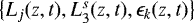 for a sufficiently long time, until it approached the time-independent case
  , which is the stationary structure we are interested in. Assuming a plane-parallel (∇ →d∕dz) and static (vgas = 0) atmosphere,Eqs. (7), (10), and (14), including the time-dependent terms, read

4.1 Closure condition
The moment Eqs. (30) and (31) are not closed because L4 appears twice on the right side, a consequence of larger particles settling faster (Eq. (6)). Therefore, a numerical solution requires a closure condition as
 (33)
(33)
We used theclosure condition explained in Appendix A.1 of Helling et al. (2008c). The idea is to approximate the particle size distribution f by a double δ-function that has four parameters. These parameters are determined by matching the given moments L0, L1, L2, and L3, and result in the fourth-moment L4 according tothe definition of the dust moments (Eq. (4)).
4.2 Operator splitting method
Figure 2 visualises our numerical approach using the operator splitting method (Klein 1995). We list the steps below.
- 1
We update Lj and
 only according to the settling source terms (the terms on the right side of Eqs. (30) and (31) containing Lj+1 and L4), applying half a time step Δt∕2, see details in Appendix B.
 - 2
We call the diffusion solver for half a time step Δt∕2 to update ɛk, and optionally, Lj and
 , if the cloud particles are to be diffused as well, see Appendix A.
 - 3
We integrate the chemical source terms (nucleation, growth, and evaporation) for a full timestep Δt. These equations are stiff at high densities and require an implicit integration scheme. We use the implicit ODE-solver LIMEX 4.2A1 (Deuflhard & Nowak 1987). The computation of the chemical source terms on the right-hand side proceeds as follows: (i) for a given temperature T, density n⟨H ⟩, and element abundances ɛk, we call the equilibrium chemistry code GGCHEM (Woitke et al. 2018) to calculate all molecular concentrations; (ii) these results are used to calculate the reaction supersaturation ratios Sr ; (iii) the nucleation rates
 and net surface reaction rates
  are determined.
 - 4
We complete the timestep by calling again the diffusion solver for Δt∕2 and the settling solver for Δt∕2 in this order.
- 5
Checkpoint and output files are written for visualisation. The method is computationally limited by the time consumption for the implicit integration of the chemical source terms, which requires numerous calls of the equilibrium chemistry. Therefore we do not split CF (Fig. 2), but set it with a full time step in the centre of the operator splitting calling sequence. The cloud formation part of the code is parallelised and can be executed for all atmospheric layers independent of each other.
 |
Fig. 2 Operator splitting calling sequence. Sett = gravitational settling, Diff = diffusion, CF = cloud formation (nucleation, growth and evaporation), and OP = output. 1/2 means half a time step, and 1 is a full time step. |
4.3 Timestep control
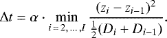
In order to produce accurate second-order solutions, the timestep must be limited to ensure that each operator remains in the linear regime. For example, the sole application of a cloud-chemistry timestep must not change the amount of dust or the element abundances substantially in any computational cell. In order to achieve code stability and accuracy, we limit the timestep as follows:
- 1
The cloud particles must not jump over layers by settling
 (34)
(34)where Δz is the vertical grid resolution and vdr,j is the mean drift velocity affecting moment ρLj, as given by Eq. (B.3). This is the usual Courant-Friedrichs-Lewy (CFL) criterion to stabilise explicit advection scheme, with an additional safety factor 1/2.
- 2
Nucleation and cloud particle growth and evaporation, as integrated over Δt, must not change any of the gas element abundances by more than a given maximum relative change (the default accuracy is 15%).
- 3
The time step must not exceed the maximum explicit diffusion timestep (Eq. (A.27)).
If one of these criteria becomes false during the simulation, the time step is discarded and Δt reduced. If the criteria are met easily, however, Δt is increased for the subsequent time step.
4.4 Boundary conditions
As our upper boundary condition, we assumed that no cloud particles settle into the model volume from above vdr,j(zmax) = 0. In the diffusion solver, we used a zero-flux (closed box) upper boundary condition, that is, the gradients of ɛk were assumed to be zero at z = zmax. The same applies to the cloud particle moments  if they are to be diffused as well.
The lower boundary was placed well below the main silicate cloud layer to ensure that the temperature was too high to allow any cloud particles to exist near the lower boundary Lj (zmin) = 0. We also demanded that the element abundances at the lower boundary equal the given values as present deep in the atmosphere 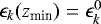 , where the
  are considered as free parameters, for example solar abundances (Asplund et al. 2009).
4.5 Initial conditions
We started all simulations from a cloud-free atmosphere Lj (z, t = 0) = 0. We experimented with two cases for the element abundances: (1) an “empty” atmosphere ɛk (z, t = 0) = 0 or (2) a “full” atmosphere  , where the index k is applied to all elements that might be transformed completely into solids (k = Si, Mg, Fe, Al, Ti, etc.), but not H, He, C, N, O, etc. For the latter elements we set
 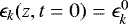 in both cases. We found an identical final structure in both cases (see Appendix C), which is very reassuring. The models calculated from initial condition (2), however, need much more computational time to complete. In this case, the nucleation rate is initially huge and a very large number of tiny cloud particles are created shortly after initialisation, which take a long time tosettle down in the atmosphere.
In order to reach the final relaxed, time-independent state, the model must be evolved until (i) the atmosphere is completely replenished several times by fresh elements ascending diffusively from the lower boundary to the very top and (ii) new grains formed high in the atmosphere have sufficient time to settle down to the cloud base and evaporate. In comparison, the chemical processes are typically quite fast. We need to evolve one model for about 106 time steps, which, depending on global parameters such as Teff and log g, translates into real evolutionary times between a few months to a few dozen years. On a parallel cluster, one such model can be completed in a few days’ time when 16 processors (about 500 CPU hours) are used, where the chemical equilibrium solver GGCHEM is called a few 109 times.
5 Results
5.1 Comparison to our previous cloud formation model
In the previous Helling & Woitke cloud formation models (Woitke & Helling 2004; Helling & Woitke 2006; Helling et al. 2008c), henceforth called the DRIFT models, the replenishment of elements was treated in a different way, using a prescribed mass-exchange timescale τmix(z) to replenish the atmosphere with fresh elements from the deep as 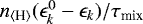 . The mass-exchange timescale was approximated by a power law logτmix(z) = const − βlogp(z) with power-law index β = 2.2 to describe convectional overshoot, see Eq. (9) in Woitke & Helling (2004). This simple approach led to an ODE-system that can be solved within about 2 CPU minutes.
Figure 3 compares the results of a previous DRIFT model with the new diffusive model, henceforth called the DIFFUDRIFT model. Both approaches model seed formation, kinetic surface growth and evaporation of cloud particles, and gravitational settling in the same way, but they differ in the treatment of the mixing that enters the cloud formation and the element conservation equations. The underlying temperature and pressure structures for all models discussed in this paper are taken from the DRIFT-PHOENIX atmosphere grid (Dehn et al. 2007; Helling et al. 2008b; Witte et al. 2009, 2011). In Fig. 3 we selected a model with effective temperature Teff= 1800 K, surface gravity log g = 3, and metallicity Z = 1 (i.e. solar abundances are assumed deep in the atmosphere). The DRIFT-PHOENIX models solve the complete 1D model atmosphere problem including convection, radiative transfer, and hydrostatic structure, coupled to our previous DRIFT model, where the cloud opacities are calculated by Mie and effective medium theory. The resulting atmosphericstructure were frozen for this study, that is, the feedback of the new cloud formation model on the (p, T)-structure was not included.
The chemical setup for this comparison has 16 elements (H, He, Li, C, N, O, Na, Mg, Si, Fe, Al, Ti, S, Cl, K, Ca), one nucleation species (TiO2), 12 solid species (TiO2[s], Al2 O3[s], CaTiO3[s], Mg2 SiO4[s], MgSiO3[s], SiO[s], SiO2[s], Fe[s], FeO[s], MgO[s], FeS[s], Fe2 O3[s]), and 60 surface reactions. The molecular setup in the new models is not quite identical because the DRIFT model uses a previous version of the chemical equilibrium solver GGCHEM, which has been replaced by the latest version (Woitke et al. 2018)in the DIFFUDRIFT model. We used 189 molecules in DRIFT and 308 molecules in DIFFUDRIFT to find the molecular concentrations in chemical equilibrium. We do not see any substantial differences in molecular concentrations caused by this data update, unless the local temperature falls below about 400 K. The thermochemical data for theselected solids are not entirely identical either, but these differences are likewise not substantial because the local temperatures remain above 700 K in this test. We assumed the mixing powerlaw index to be β = β′ = 1 for both τmix(z) in DRIFT and Dgas(z) in DIFFUDRIFT, see Eq. (18) and Fig. 1, although the meaning of β and β′ is slightly different. We note that using β′ > β would likely produce results that are more similar to each other than those presented in this paper. The lower volume boundary for the size integration of the cloud particle moments was set to Vℓ = 10 × VTiO2, where VTiO2 = 3.14 × 10⁻²³ cm3 is the assumed volume of one unit of solid TiO2[s].
The resulting cloud structures, as predicted by our previous DRIFT and the new DIFFUDRIFT models, are compared in Fig. 3. The diffusive transport of condensable elements up into the high atmosphere with DIFFUDRIFT is much less efficient than the assumed replenishment in the DRIFT model. As these elements are slowly mixed upwards by diffusion, they can collide with existing cloud particles to condense on, and hence far fewer of these elements reach the high atmosphere where the nucleation takes place. This is the main difference between the DRIFT and the DIFFUDRIFT models. In the previous DRIFT models, the mixing process was assumed to take place instantly.
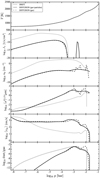 |
Fig. 3 Comparison of cloud formation models for Teff = 1800 K, log g =3, metallicity Z = 1, and β = β′ = 1. The previous DRIFT model is shown by the thick grey lines. Two DIFFUDRIFT models are overplotted assuming pure gas diffusion (dashed lines) and gas + particle diffusion (black solid lines). dust/gas = ρdL3 is the dust-to-gas mass ratio, nd = ρL0 the number density of cloud particles, |

Cloud structure
Consequently, the new DIFFUDRIFT model is featured by up to five orders of magnitude lower nucleation rates (Fig. 3) and less cloud particles high in the atmosphere. At intermediate pressures (10−6... 10−3 bar), we find that the fewer cloud particles in the DIFFUDRIFT model grow quickly and reach particle sizes of about 10 μm at 1 mbar, whereas in the DRIFT model, the cloud particles remain smaller, about 0.3 μm, because there are so many of them. The growth of the cloud particles is limited by the amount of condensable elements available per particle, and therefore, this effect is expected.
The dust-to-gas mass ratio, ρd∕ρgas, increases more steeply in the DIFFUDRIFT model, but reaches about the same maximum of order 10−3 at 1 mbar as in the DRIFT model. Thus, overall, the cloud formation process is about equally effective, but the clouds are spatially more confined in the DIFFUDRIFT model, reaching up just a few scale heights above the cloud base.
Table 2 lists vertically integrated cloud column densities for the three models. We find values of a few milligrams of condensates per cm2, where the DIFFUDRIFT model without cloud particle diffusion is found to be the most dusty one. When an order of magnitude estimate of cloud particle opacities (see Appendix E) is used, values between several 100 cm2 g−1 to several 1000 cm2 g−1 at λ= 1μm are expected, depending on material and particle size distribution, that is, a column density of 1 milligram of condensate per cm2 roughly corresponds to an optical depth of one at λ = 1 μm. This impliesthat all three models discussed here have optically thick cloud layers.
The computation of more realistic cloud particle opacities will need to take into account the height-dependent material composition, size distribution, and possibly the shape of the cloud particles, as done, for example, by Dehn et al. (2007), Witte et al. (2009, 2011) and Helling et al. (2019). In comparison to the previous DRIFT models, the particles in the DIFFUDRIFT models are larger, which is likely to cause the optical depths to be somewhat smaller, although the cloud mass column densities are similar. In addition, molecular opacities need to be added to calculate the spectral appearance of the objects and feedback onto the (p, T)-structure, which goes beyond the scope of the present paper.
The resulting particle properties in the main cloud layer below 1 mbar depend not only on the treatment of mixing, but also on whether we switch on the dust diffusion in the DIFFUDRIFT model. In this region, the cloud particles stepwise purify chemically as they decent in the atmosphere (see Fig. 5). Thermodynamically less stable materials such as Fe2 O3[s], FeO[s], and FeS[s] sublimate off the cloud particles sooner. Subsequently, the abundant magnesium-silicates MgSiO3[s] and Mg2SiO4[s] sublimate as well, which causes the cloud particles to shrink significantly around 1 mbar. Close to the cloud base, at about 1800 K in this model, only the most refractory materials remain, in particular metal oxides such as Al2 O3[s], CaTiO3[s] and TiO2[s], before even these materials eventually sublimate and the cloud particles evaporate completely.
As one material sublimates, the liberated elements may re-condense into different condensates, which are thermodynamically more stable, leading to rapid changes in particle size and material composition. There is also a dynamical effect. When the particles shrink, their fall speeds decrease, which leads to spatial accumulation, hence the number density of cloud particles nd increases. While these effects and the general behaviour of the cloud particles are similar in all three models, the steps of sublimation are more pronounced in the DIFFUDRIFT model without dust diffusion. Dust diffusion tends to smooth out the variations of particle size and density.
Element abundances
Figure 4 compares the resulting gas element abundances. We see a strong depletion of condensable elements in the main cloud layer in all three models, by up to five orders of magnitude, concerning elements Ti, Al, Mg, Si, Mg, and Fe. However, the details are different. The previous DRIFT model is featured by minimums of ɛk that are similar in depth as compared tothe overall decrease of ɛk in the DIFFUDRIFT models. High up in the atmosphere, where cloud particles are virtually absent, there is no surface to condense on, and so the instantaneous mixing assumption in the DRIFT models causes a re-increase of ɛk toward the top of the atmosphere, unless the element can form nuclei. In the extremely low density gas at these heights, the nuclei simply fall through the atmosphere without much interaction, whereas elements that cannot nucleate, accumulate.
In contrast, in the new DIFFUDRIFT models, the abundances of all elements involved in cloud formation decrease with height in a monotonic way. This behaviour is expected in the final, time-independent, relaxed state of the atmosphere, as discussed in Sect. 3.1. In the stationary case, the downward transport of condensable elements via the falling cloud particles must be compensated for by an upward diffusive transport of these elements in the surroundinggas, which implies negative element abundance gradients throughout the cloudy atmosphere, see Eq. (29). The total drop of element abundances is deepest for Ti, but more shallow for Si and Fe than for Mg.
Freytag et al. (2010) performed 2D radiation hydrodynamical simulations of substellar atmospheres that included a time-dependent description for the formation of a single type of cloud particles for a fixed concentration of seed particles. The authors discussed substellar objects with Teff = 900−2800 K, log(g) = 5 and solar element abundances. Their Fig. 9 (bottom left panel) shows the fraction of condensable gas in the atmosphere as a function of pressure, very similar to our Fig. 4 (lower plot). These results of Freytag et al. (2010) support our new DIFFUDRIFT results, where abundances of condensable elements in the gas phase decrease fast in the cloud layers and remain about constant above the clouds. We note that Freytag et al. (2010) prescribed the number of seed particles and considered only one generic condensate in their simulations.
 |
Fig. 4 Effect of our assumptions on the mixing processes in the atmosphere on the resulting gas element abundances, in models with the same parameters as in Fig. 3. Upper plot:
|

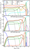 |
Fig. 5 Material volume composition of the cloud particles |
Cloud particle composition
Figure 5 shows the corresponding solid material composition (by volume) of the cloud particles. In all three models we assumed that the cloud particles have a well-mixed material composition that is independent of size, but that composition changes as the particles fall through the atmosphere, hence material composition depends on height. All three models show the same basic vertical structure.
- 1
A layer containing only the most stable metal-oxides at the cloud base, in this model Al2 O3[s], TiO2[s], and CaTiO3[s]. The position of the cloud base, which depends on Teff and log g, is located ataround 1800 K in this model.
- 2
A thin layer of cloud particles around 1500 K that mainly consist of metallic Fe[s].
- 3
Main silicate cloud layer composed of Mg2 SiO4[s], MgSiO3[s], MgO[s], SiO[s], and SiO2[s], mixed with metallic iron, upward of about 1400 K in this model.
- 4
Lessstable solid materials such as FeS[s], FeO[s], and Fe2 O3[s] are incorporated into the silicate cloud particles at temperatures lower than about 1100 K, 1000 K, and 850 K, respectively, in this model.
- 5
Pure nuclei at the top, here TiO2[s], which fall through the atmosphere so quickly that they practically do not grow.
Further inspection shows, however, that the material composition of the main silicate cloud layer (3) differs substantially between the DRIFT and the DIFFUDRIFT models. In the new diffusive DIFFUDRIFT models, the first magnesium-silicate to form is fosterite Mg2 SiO4[s], which has a stoichiometric ratio Mg : Si = 2 : 1. The formation process of Mg2 SiO4[s] stops when the reservoir of Mg is exhausted, still leaving about half of the available Si in the gas phase. Because the mixing is diffusive, very little Mg can be mixed upwards through these Mg2 SiO4[s] clouds. Thus, the remaining amount of Si above the Mg2 SiO4[s] clouds preferentially forms other silicate materials, in particular SiO2[s] and SiO[s], but only very little MgSiO3[s]. This is different in our previous DRIFT model, where the depleted elements are assumed to be instantly replenished at similar rates, in which case both Mg2 SiO4[s] and MgSiO3[s] are found to be about equally abundant condensates in the main silicate cloud layer.
Another difference concerns FeS[s] (troilite). FeS[s] is found to form in large quantities in the previous DRIFT models, causing ɛS to drop significantly, see the upper part of Fig. 4. However, this depends on our assumptions about how the elements are replenished. In the new diffusive models, upward mixing of gaseous Fe is rather inefficient because the Fe atoms have many opportunities to condense in form of Fe[s] on existing cloud particles along their way upwards in the atmosphere. When the temperature is low enough to allow FeS[s] to form, so little Fe is left in the gas phase that the S abundance is more or less unaffected by FeS[s] formation, and therefore sulphur remains available for other condensates to form.
5.2 Cloud structures as a function of Teff
In this section, we study the results of a sequence of the new DIFFUDRIFT cloud formation models with decreasing effective temperature Teff. We used a slightly different chemical setup here that allows us to discuss secondary cloud layers. We considered four nucleation species  ,
,  ,
,  , and
, and  . The nucleation rates of TiO2, KCl, and C were calculated by modified classical nucleation theory (Helling et al. 2017; Gail et al. 1984), with a surface tension value for KCl from Lee et al. (2018). The nucleation rate of SiO is calculated according to Gail et al. (2013). We included 16 elements in this setup (H, He, Li, C, N, O, Na, Mg, Si, Fe, Al, Ti, S, Cl, K, and Ca), 14 condensed species (TiO2[s], Al2 O3[s], MgSiO3[s], Mg2 SiO4[s], SiO[s], SiO2[s], Fe[s], FeS[s], FeO[s], MgO[s], KCl[s], NaCl[s], Na2S[s], and C[s]), 308 molecules and 50 surface growth reactions. Molecular equilibrium constants and Gibbs free energies of the condensates were all taken from Woitke et al. (2018). Dust diffusion was included in all models.
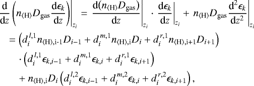
Figure 6 shows the total column densities of selected cloud materials Σs [g cm−2] in a series of DIFFUDRIFT models with constant logg = 3 and mixing index β′ = 1, but decreasing Teff. The column densities of the condensed species were computed as
 (35)
(35)
where ρs [g cm−3] is the material density of the pure condensate of kind s and ![Mathematical equation: $\rho L_3^s\rm\,[cm^3\,cm^{-3}]$](/articles/aa/full_html/2020/02/aa36281-19/aa36281-19-eq70.png) is the volume of condensed kind s per volume of atmosphere. For example, for Teff = 1800 K we find about 10 mg condensates per square centimetre, mostly made of Mg2SiO4[s], Fe[s] and Al2O3[s], followed by SiO[s] and MgSiO3[s].
is the volume of condensed kind s per volume of atmosphere. For example, for Teff = 1800 K we find about 10 mg condensates per square centimetre, mostly made of Mg2SiO4[s], Fe[s] and Al2O3[s], followed by SiO[s] and MgSiO3[s].
On the left side of this plot, the first model that shows condensation appears at Teff= 2800 K. Here, the temperatures are too high for condensates other than just the most stable metal oxides in form of Al2O3[s] and TiO2[s]. In the next few models down to Teff = 2000 K, the main silicate layer forms, mixed with iron. In this range of effective temperatures, Al2O3[s] still has the highest column density because the metal-oxide layer is situated deeper in the atmosphere where the densities are higher. Only for Teff < 2000 K does the silicate-iron layer start to dominate by mass. At the very end of the sequence, for Teff < 1500 K we find the first models that host a third cloud layer made of di-sodium sulfide Na2S[s].
Figure 7 shows a few more details from this Teff series of new cloud formation models. The upper left plot shows the atmospheric density and temperature structures we assumed, taken from the DRIFT-PHOENIX atmosphere grid (Dehn et al. 2007; Helling et al. 2008b; Witte et al. 2009, 2011). The kinks in deep layers (T ~ 2500−3000 K) indicate the beginning of the convective layer (Schwarzschild criterion for convective instability). The upper right plot shows the assumed diffusion coefficient in the atmosphere, which decreases with Teff, because the convective layer sinks into deeper layers, hence the spatial distance to the source, which causes the mixing motions in the atmosphere, increases.
The left middle plot in Fig. 7 shows the dust-to-gas mass ratio, which has its maximum in the main silicate-iron layer, and a shoulder on the right caused by the deeper metal-oxide clouds, which are made of the rarer elements with the highest condensation temperatures: aluminium, calcium, and titanium. As Teff decreases, both layers move inward to deeper layers and become successively more narrow, until finally, for Teff = 1400 K, a new cloud layer occurs that mainly consists of di-sodium sulfide Na2S[s]. The right middle plot shows the effect on the silicon abundance in the gas phase. All curves decrease monotonically towards the surface, with higher Si depletions for lower Teff where the silicate cloud particle formation is more complete.
The nucleation rates of  and
and  particles are depicted in the lower left plot. A complicated double-peaked pattern emerges that has a minimum around the main peak of the dust-to-gas ratio (at the peak position of the main silicate-iron layer).
  is usually the most significant nucleation species, but cooler models show additional contributions by
  . The resulting mean particle sizes are plotted on the lower right, with a tendency to produce larger particles deep in the atmosphere for lower Teff. An in between minimum in particle size occurs where the main silicate material evaporates. Only the coolest model has a second minimum where Na2S[s] evaporates. Interestingly, the hottest and coolest models in Fig. 7 show about equally large cloud particles at high altitudes, whereas all other models show smaller particles.
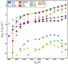 |
Fig. 6 Column densities [g cm−2] of different condensates in the atmosphere for a sequence of models with decreasing Teff but constant logg = 3 and β′ = 1. A value of 10−3 g cm−2 roughly corresponds to an optical depth of one at a wavelength of λ = 1 μm (see Appendix E). |
6 Summary and discussion
This paper has introduced a new cloud formation model that is applicable to the atmospheres of brown dwarfs and gas giant (exo-)planets. We combined our previous cloud particle moment method (Woitke & Helling 2004; Helling & Woitke 2006; Helling et al. 2008c) with a diffusive mixing approach, according to which fresh condensable elements are diffusively transported upwards to replenish the upper atmosphere via a combination of turbulent (eddy) mixing and gas-kinetic diffusion in the final relaxed time-independent state of the atmosphere. Our formulation of the problemarrives at a system of about 30 second-order partial differential equations of reaction-diffusion type, where the formation and growth of the cloud particles follows from a kinetic treatment in phase-non-equilibrium.
Model setup
The new cloud formation model was applied to a given 1D (p, T) atmosphericstructure in this paper. The model was calculated time-dependently, using an operator splitting technique. All models are found to relax toward a time-independent stationary solution, where the condensable elements are constantly mixed up diffusively, cloud particles nucleate from the gas phase high in the atmosphere, grow by the simultaneous condensation of different solid materials on their surface, and then descent through the atmosphere due to gravitational settling, before the particles stepwise purify and eventually sublimate completely at the cloud base.
Timescales
The real-time simulation time required to reach this stationary solution varies between a few months to several dozen years, depending on log(g) and Teff. The relaxation is quicker when models are started from an atmosphere that is devoid of any condensable elements at t = 0. These relatively long simulation times make the models computationally expensive (about 500 CPU-hours per model) because the intrinsic nucleation and growth reactions are very fast, which means that the models need to be advanced on short computational time steps of the order of seconds to guarantee numerical stability. The long physical timescales involved in the simulations are (i) the overall settling time for small particles inserted high in the atmosphere, and (ii) the overall mixing time for gas parcels to diffusively reach the highest point in the model from the cloud base. This implies that 3D simulations of cloud formation (GCM models, e.g. Freytag et al. 2010; Lee et al. 2016; Lines et al. 2018; Powell et al. 2018; Charnay et al. 2018) must be advanced for similar real-time simulation times before a relaxed physical structure can be expected. However, how long these physical timescales actually are will depend on the exact formulation of mixing and setting in the GCM models.
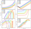 |
Fig. 7 Sequence of cloud forming models with decreasing Teff at constant logg = 3 and mixing power-law index β′ = 1. Top row: gastemperature T and diffusioncoefficient Dgas as a functionof pressure (both assumed). Middle row: resulting dust-to-gas mass ratio and element abundance of silicon in the gas phase ɛSi. Lower row: resulting nucleation rates J⋆ and mean particle sizes |

Cloud density and particle sizes
In comparison to our previous DRIFT models, the DIFFUDRIFT models show fewer but larger cloud particles, which are more concentrated towards the cloud base. However, the physical properties of the cloud particles in the main silicate-iron layer towards the bottom of the clouds (dust-to-gas mass ratio, particle sizes, optical depth, chemical composition, etc.) are found to be similar to the results of the previous models. The dust-to-gas ratio in the main silicate-iron layer reaches a peak value of about 0.002 to 0.003, quite independent of Teff, for moderately hot models (Teff > 2500 K). This is close to the maximum value of 0.0045 that is expected from complete condensation of a gas with solar abundances (Woitke et al. 2018). The physical reason for the stronger concentration of the cloud particles around the cloud base in the DIFFUDRIFT models is that the diffusive element replenishment is less effective for the upper atmosphere because the molecules carrying the elements diffusively upwards have a high probability of colliding with existing cloud particles on their way up the atmosphere. This effect was not accounted for in our previous models.
Element abundances
The concentration of condensable elements in the gas phase shows a steep decline in the DIFFUDRIFT models above the cloud base, followed by a monotonous decrease towards a plateau that continues on that level toward the upper boundary of the model. This behaviour is expected in the time-independent relaxed state because the downward flux of condensable elements via the falling cloud particles must be compensated for by an upward diffusive flux of elements in the gas phase. This in turn requires a negative concentration gradient. We find that the abundances of the condensable elements high above the cloud layers strongly depend on effective temperature, in agreement with the results of 2D radiation hydro-models by Freytag et al. (2010). For example, the silicon abundance is reduced by about 2.5 orders of magnitude for Teff = 2000 K, but by 6 orders of magnitude for Teff = 1300 K in our models.
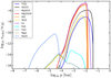 |
Fig. 8 Concentration of condensed species in a model with Teff = 1300 K,
log g =3, and β′ = 1, showing a secondary cloud layer almost entirely made of di-sodium sulfide Na2 S[s]. |
![Mathematical equation: $n^s_{\textrm{cond}}=\rho L_3^s/V_{\textrm{mat}}^s\rm\,[cm^{-3}]$](/articles/aa/full_html/2020/02/aa36281-19/aa36281-19-eq137.png)

Cloud material composition
The chemical composition of the cloud particles is characterised by (i) a deep layer with only the most stable metal oxides at the cloud base (Al2 O3[s], TiO2[s], and CaTiO3[s] in the current setup), (ii) the main silicate-iron layer (Mg2SiO4[s] and Fe[s]), which is enriched by other silicates such as SiO[s] and SiO2[s] and MgSiO3[s] at increasing heights. Some less stable condensates are also found in smaller quantities, in particular FeS[s] and FeO[s]. The condensation in both these cloud layers leads to a removal of certain elements from the gas phase, and the stoichiometry of the condensates decides upon which elements remain for further condensation higher in the atmosphere. In particular, the formation of Mg2 SiO4[s], with stoichiometry Mg : Si = 2 : 1, causes the Mg abundance to drop quickly, whereas roughly half of the originally available Si remains in the gas phase. This then favours the formation of SiO[s] and SiO2[s] above the Mg2 SiO4[s] layer, rather than the formation of MgSiO3[s], which is a rather unimportant condensate in our new DIFFUDRIFT models. The low abundance of MgSiO3[s] in the main silicate-iron layer is a result that differs from the results obtained with our previous DRIFT models, and from phase-equilibrium models starting from complete solar abundances (Woitke et al. 2018).
Na2S[s] clouds
Our coolest DIFFUDRIFT models show the occurrence of a secondary cloud layer almost entirely made of di-sodium sulfide Na2 S[s], see Fig. 8. The presence of Na2S-clouds in brown dwarf atmospheres has been proposed by Morley et al. (2012) to fit the optical appearance of two red T dwarfs. The formation of Na2 S-clouds requires the presence of sulphur and sodium in the gas phase at low temperatures. In phase-equilibrium models starting from solar abundances,this combination is prevented by the formation of FeS[s] (troilite), which consumes the sulphur. However, in our new diffusive kinetic cloud formation models, iron is depleted by the formation of metallic iron Fe[s] at high temperatures, so that FeS[s] cannot form in large quantities. Consequently, sulphur remains available to eventually form Na2 S[s] at lower temperatures. The condensation of Na2S[s] then reduces the possibility of forming NaCl[s] at even lower temperatures, and so on. Therefore, the new diffusive DIFFUDRIFT models reveal new details about the condensation sequence in cloudy atmospheres, and we need more experiments with our selection of condensates during model initialisation to arrive at more distinct conclusions.
7 Conclusions
The physical description of the replenishment mechanism for condensable elements in planetary atmospheres seems crucial for realistic cloud formation models. This paper has used a quasi-diffusive approach in 1D to simulate the turbulent eddy-mixing processes in cloudy atmospheres, using the new DIFFUDRIFT models. This approach can be considered as the limiting case of small-scale mixing. At the other extreme, large-scale hydrodynamic motions (convection, Hadley cells, etc.) might be able to dredge up these elements in a possibly more direct way, which was the idea in our previous DRIFT models. In reality, there is not only vertical, but also horizontal mixing, which is likely to be quite fast, for example in super-rotating horizontal jets as known from Jupiter (Schneider & Liu 2009). However, horizontal mixing alone cannot couterbalance vertical settling on the long run, it rather stimulates vertical mixing via e.g. Kelvin-Helmholtz instabilities. More 3D numerical experiments are required to quantify the efficiency of mixing to inform our cloud formation models.
Acknowledgements
Ch.H. thanks Will Best and Jonathan Gagné for the discussion on the number of known brown dwarfs. We thank Robin Baeyens and Ludmila Carone for insightful discussions on mixing regimes in gas giant planets. The computer simulations were carried out on the UK MHD Consortium parallel computer at the University of St Andrews, funded jointly by STFC and SRIF.
Appendix A Diffusionsolver
We used a self-developed 1D explicit/implicit diffusion solver in this paper that has second-order accuracy in both the formulation of the differential equations and the boundary conditions3. In case of a plane-parallel static atmosphere, the diffusion equation for element k is given by
 (A.1)
(A.1)
where the diffusive element flux is
 (A.2)
(A.2)
A.1 Vertical grid and discretisation of derivatives
We introduce an ascending vertical grid zi (i = 1,..., I). The first and second derivatives of any quantity f(zi) = fi at grid point zi are approximated as

that is, as linear combinations of the function values on the neighbouring grid points, where  , for example, is the coefficient for the first derivative on the point left of the grid point i,
  the same on the mid-point, and
  the same on the point right of grid point i. Similar, for the second derivative, the coefficients are
  ,
,  and
and  . When we use a second-order polynomial approximation for function f(z), the coefficients are given by

where  and
and  are the left- and right-hand side grid point distances. For the special case of an equidistant grid, we have
  and hence

The above equations are valid for grid points i = 2,..., I − 1. For the first derivative at the boundaries, we write

which is also second-order accuracy by using the information on the three leftmost or three rightmost grid points, respectively. The coefficients are given by

where h2 = z2 − z1, h3 = z3 − z1, hI−1 = zI − zI−1, and hI−2 = zI − zI−2.
A.2 Spatial derivatives
The diffusion term at grid point zi (i = 2... I − 1) is numerically resolved, with abbreviation Dgas(zi) = Di, as
 (A.21)
and the diffusive fluxes across the lower and upper boundaries are

A.3 Boundary conditions
As boundary conditions, we implemented three options, for example considering the lower boundary:
- 1.
fixed concentration: ɛk,1 is a given constant;
- 2.
fixed flux: ϕk,1 is a given constant;
- 3.
fixed outflow rate: the flux through a boundary is assumed to be proportional to the concentration of species k at the boundary, for instance,
![Mathematical equation: \begin{eqnarray*} \phi_{k,1} = \beta_k\,n_{\langle{\textrm{H}}\rangle,\textrm{1}}\,\epsilon_{k,1}\,\textrm{v}_k \quad\quad{\rm[cm^{-2}s^{-1}]}, \end{eqnarray*}](/articles/aa/full_html/2020/02/aa36281-19/aa36281-19-eq93.png) (A.24)
(A.24)
where βk is a given probability (fixed value)and vk is the speed at which element k moves through the boundary (also fixed value).
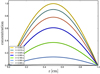 |
Fig. A.1 Test problem with fixed concentrations on the left and right boundaries (ɛ = 0). The thin black lines overplot the analytic solution ɛ(z, t) = exp(−ωt)sin(kz) with k = π and ω = Dk2. |
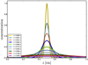 |
Fig. A.2 Diffusive evolution of an initial δ peak with analytic solution overplotted. The analytic solution is |

A.4 Explicit integration
A straightforward way to integrate Eq. (A.1) for a time step Δt is the following explicit scheme:
 (A.25)
where  is some quantity on grid point i at time tn and
  is the quantity on grid point i at time tn−1 with tn = tn−1 + Δt. In consideration of Eq. (A.1), this leads to
 (A.26)
where A is a tri-diagonal matrix, the elements Aij of which are given by Eq. (A.21). Equation (A.26) applies to the grid points i = 2,..., I − 1, but not to the boundaries. On the boundary points, the following equations are applied depending on the choice of boundary conditions, here for example the lower boundary,
- 1.
fixed concentration:

- 2.
fixed flux:
- 3.
fixed outflow rate:

These assignments are applied at time tn, that is, after an explicit diffusion time step has been completed on grid points i = 2... I − 1. To guarantee numerical stability, the explicit time step must be limited by α ≤ 0.5 according to
 (A.27)
A.5 Implicit integration
To avoid the time-step limitations in the explicit solver and to guarantee numerical stability for much larger time steps, an implicit integration scheme can optionally be applied,
 (A.28)
which is a system of linear equations for the unknowns  . In consideration of Eq. (A.1), we have
 (A.29)
We re-write this equation more generally, including the boundary conditions, by means of another unit-free matrix as
 (A.30)
where we have
 (A.31)
where some of the Bij and Rk,i depend on the selected boundary conditions, for example at the lower boundary,
- 1.
fixed concentration: B11 = 1 and

- 2.
fixed flux: B11 = 1,
 ,
,
 , and
, and
- 3.
fixed outflow rate:
 ,
,
 ,
,
 , and Rk,1 = 0.
We can now perform an implicit time step according to Eq. (A.30) as
 (A.32)
where B−1 is the inverse of the matrix B. As long as the spatial grid points zi, the densities n⟨H ⟩,i and diffusion constants Di, the constants involved in the boundary conditions (e.g. ϕk,1 or βk), and the time step Δt do not change, we need to perform the matrix inversion only once. Successive time steps are then performed by simply incrementing n, re-computing the vector Rk, and applying again Eq. (A.32). B−1 is also usually the same for all elements k to be diffused.
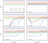 |
Fig. A.3 Testing the model convergence for different initial conditions: gas element abundances ɛk as a functionof pressure p in two cloud formation models with different initial conditions, “empty” (left) and “full” (right), see text for further explanations. Panels from top to bottom: respective results after t = 0, t = 10 days, and t = 8000 days. |
This favourable property of B makes the computation of implicit time steps very fast. We note, however, that B−1 is in general a full I × I matrix where all entries are positive  . This leads to a very stable numerical behaviour for arbitrary time steps. In contrast, the matrix A has positive entries along the main diagonal, but negative entries along both semi-diagonals, which leads to numerical instabilities when the time step is too large.
Appendix B Settling solver
For the 1D vertical settling in the Epstein regime we solve
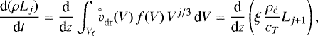 (B.1)
(B.1)
according to Eqs. (6) and (8). The settling flux for cloud particle moment ρLj is hence
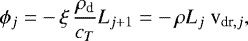 (B.2)
(B.2)
where we have introduced mean drift velocities for the cloud particle moments ρLj as
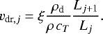 (B.3)
(B.3)
The cloud particle moments are updated according to the following explicit upwind advection scheme. We first calculate all vertical moment fluxes ϕj,i = ϕj(zi) via Eq. (B.2) and then apply

where the notation  is some quantity on grid point i at time tn, Δt = tn − tn−1 the time step, and Δz the vertical extension of the considered atmospheric cell.
Appendix C Verification tests
We carefully checked our diffusion solver against analytical test problems and by cross-checking the results from the explicit and implicit solvers. Figures A.1 and A.2 show two test problems in the domain z = [0, 1], with constant n⟨H⟩ = 1 and D = 1. The black thin lines are the overplotted analytic solutions, showing excellent agreement. The tests use an equidistant z-grid with 101 points, and can be computed within less than 1 CPU second.
The convergence of the full cloud formation model was studied by comparing the results obtained with different initial conditions (see Sect. 4.5). Figure A.3 shows the results of two models for Teff = 1800 K, log g = 3, β′ = 1, and solar abundances. The initially “full” model shows a massive cloud formation event just after onset. The cloud formation is most effective at high densities and low temperatures, causing transient minimums of ɛk (z). The initially “empty” model needs more time to start forming clouds because the condensable elements first need to be transported upwards by diffusion, resulting in a more gradual onset of cloud formation. The final states after t = 8000 days are identical in both cases, where the ɛk(z) decrease monotonically with height and have zero gradients at the upper boundary, as expected in the time-independent case, see Sect. 3.1.
Appendix D Diffusion coefficients in the literature
Diffusion is in principle a microscopic process driven by particle concentration gradients ∇cj, where for example cCO = nCO∕ntot for j = CO and ntot = ∑ nj is the total particle density. Gradients like this can result from gravity (Zahnle et al. 2016), from chemical processes (Moses et al. 2000), and from cloud condensation, as shown in this paper. Diffusion will always counteract these concentration gradients. Experiments have been conducted to measure diffusion constants for gases relevant for Solar System planets. Lamb & Verlinde (2011), for example,provided the gas-kinetic diffusion coefficient for water molecules near sea level in the Earth atmosphere (DH2O ≈ 2 × 10⁻¹ cm2 s−1) and noted that it varies inversely proportional with the atmospheric pressure.
The effect of mixing on larger scales has been modelled differently in different communities, and the terminology is usually not unique. Often, a quasi-diffusive approach is used where the diffusion constant is replaced by a function of height, of density, or of pressure. Transport of matter due to turbulent mixing has been termed “turbulent diffusion” in protoplanetary disc modelling, describing the averaged effect of advection of the individual turbulent eddies (e.g. Schräpler & Henning 2004) and as “eddy diffusion” inplanetary atmosphere modelling.
Studying Solar System gas giants, Moses et al. (2000) have demonstrated that ISO observations of hydrocarbon molecules in Saturn’s atmosphere can be well fitted by assuming an eddy diffusion coefficient of
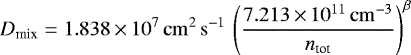 (D.1)
(D.1)
with slope β between 0.3 and 0.7, that is, Dmix increases with height.
Ackerman & Marley (2001) considered an equilibrium between upward mixing of vapour in the gas phase and gravitational settling of particles condensed from the vapour. Their Eq. (4) reads
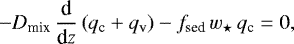 (D.2)
(D.2)
where qv and qc are the mixing ratios of vapour and condensate, respectively (moles of vapour and condensate per mole of atmosphere). fsed w⋆ represents an average sedimentation velocity of the condensed particles with fsed being adjusted as needed. We note that Eq. (D.2) is very similar to our Eq. (29) for the case where cloud and gas particles are equally affected by eddy diffusion. Their eddy-diffusion coefficient Dmix is defined according to Gierasch & Conrath (1985) as
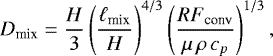 (D.3)
(D.3)
where H = RT∕(μ g) is the pressure scale height, ℓmix the mixing length, cp = (f + 2)R∕(2μ) is the isobaric specific heat, f is the mean degree of freedom of the gas particles, R is the universal gas constant, and Fconv is the convective heat flux. Ackerman &Marley (2001) assumed  , that is, they assumed that the atmosphere is fully convective, which leaves open the problem of what to do in radiative layers, for example in brown dwarfatmospheres. Charnay et al. (2018) noted that the factor 1/3 was chosen to match observations from gas giant planets. The mixing length lmix is calculatedas
 (D.4)
(D.4)
in Ackerman & Marley (2001), where Γ and Γadb are the local and dry adiabatic lapse rates, respectively, and Λ is the minimum scaling applied to ℓmix, chosen to be 0.1. The average sedimentation velocity is w⋆ = Dmix∕ℓmix. We note that if H, cP and ℓmix are constants, the diffusion constant scales as 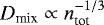 in the Ackerman & Marley models, that is, their Dmix increases with height. Charnay et al. (2018) used a similar approach, deriving the convective heat flux from their simulations inside the convective zone. In radiative layers, however, they assumed
 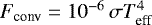 to account for the effect of convective overshooting. This approach enabled them to model secondary cloud layers.
Zahnle et al. (2016) used a combination of gas-kinetic diffusion and eddy diffusion, which is standard in 1D chemical models for planetary atmospheres,

Here, bia = Dia∕ntot [cm−1 s−1] is the binary diffusion coefficient and Dia [cm2 s−1] is the gas-kinetic diffusion coefficient for particles of kind i in a background atmosphere a with mean molecular weight μ. Pi and Li [cm−3 s−1] are the chemical production and loss rates, and ϕi [cm−2 s−1] is the total diffusive flux of particles of kind i. It is straightforward to verify that, in the absence of chemical processes and eddy diffusion, molecules of different kinds i would eventually relax towards independent stratifications ni = ni,0 exp(−z∕Hi) with scale heights Hi = kT∕(mi g), whereas the background atmosphere would follow ntot = ntot,0 exp(−z∕H) with H = kT∕(μ g). This effect could be described as “gravitational de-mixing”, resulting from the action of the force of gravity on a mixture of gases when only gas-kinetic diffusion is active. Conversely, eddy diffusion counteracts this tendency and tends to homogenise the concentrations. The critical level below which the atmosphere is well mixed is called the homopause and follows from Dia (z) = Dmix(z). In their models, Dmix is a free constant between (105−1010) cm2 s−1. We note that when the first term in Eq. (D.6) is neglected, this matches our approach (Eq. 14) with Dgas = Dmix + Dmicro. A similar description has been used by Rimmer & Helling (2016, see their Eq. (23)).
Using 2D radiative-hydrodynamics simulations for brown dwarf atmospheres, Freytag et al. (2010, see their Sect. 4.3 and Figs. 13 and 14) estimated eddy-diffusion coefficients from root-mean-square gas velocities ⟨v⟩ as found in their models. Results range from about 105 to 109 cm2 s−1, depending on the details of the conversion formula applied, and are relatively constant throughout the atmosphere.
Parmentier et al. (2013, see their Eq. (22)) followed tracer particles in their 3D GCM models for the hot Jupiter HD 189733b to provide approximate eddy-diffusion coefficients as a function of gas pressure as
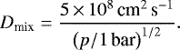 (D.7)
(D.7)
Using a different 3D GCM code with time-dependent cloud formation theory for HD 189733b, Lee et al. (2015a) provided approximate eddy-diffusion coefficients (their Fig. 3) fitted with a power law as Dmix ∝ p−0.65, again showing increasing eddy-diffusion coefficients with height.
Zhang & Showman (2018) used 3D atmosphere models to study tracer particles that have a certain (chemical) lifetime. They suggested Dmix ~ τc when the chemical lifetime τc of a tracer species is short and Dmix is constant. Regime-dependent Dmix parametrisations are provided.
Other parametrisations are used in modelling planet-forming discs. In Zsom et al. (2011), the parametrised diffusion coefficient is
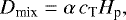 (D.8)
(D.8)
where α is the dimensionless viscosity parameter introduced by Shakura & Sunyaev (1973),
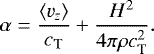 (D.9)
(D.9)
When magnetic fields H are neglected, then Eq. (D.8) reduces to our Eq. (17) for the eddy-diffusion coefficient. α ≈ 10−6−10−2 is treated as an adjustable parameter in disc simulations. In Youdin & Lithwick (2007), the gas diffusion coefficient takes the form
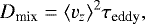 (D.10)
where τeddy is the turbulent eddy turnover timescale.
Appendix E Cloud opacity estimations
As an order-of-magnitude estimate for cloud particle opacities, we considered small spherical particles with optical constants for astronomical silicates (Draine & Lee 1984; Laor & Draine 1993), using a MRN (Mathis et al. 1977) size distribution f(a) ∝ a−3.5 between amin = 0.005 μm and amax = 0.25 μm, which is standard for the dust in the interstellar medium. Opacities were calculated by Mie theory and are listed in Table E.1.
Cloud opacities in the atmospheres of brown dwarfs and exoplanets will differ from those values because of deviations in material composition, size, and shape distribution. Typical opacity values for larger particles in protoplanetary discs at λ = 1 μm are expected to range from several 100 to several 1000 cm2 g−1(dust), see for example Fig. 3 in Woitke et al. (2016).
Based on the total column densities of cloud particles found in our models (see Table 2 and Fig. 6), we conclude that the clouds in our models are increasingly optically thick towards lower effective temperatures. We estimate that the clouds become optically thick at λ = 550 nm for Teff ≲2500 K, at λ = 1 and 10 μm for Teff ≲2000 K, but are considerably more transparent at λ = 5 μm and beyond λ≳30 μm.
MRN astronomical silicate dust extinction opacities  for selected wavelengths λ, see text for references.
References
- Ackerman, A. S., & Marley, M. S. 2001, ApJ, 556, 872 [NASA ADS] [CrossRef] [Google Scholar]
- Allard, F. 2014, IAU Symp., 299, 271 [NASA ADS] [Google Scholar]
- Allard, F., Homeier, D., & Freytag, B. 2012, Phil. Trans. R. Soc. London, Ser. A, 370, 2765 [Google Scholar]
- Apai, D., Radigan, J., Buenzli, E., et al. 2013, ApJ, 768, 121 [NASA ADS] [CrossRef] [Google Scholar]
- Arcangeli, J., Désert, J.-M., Line, M. R., et al. 2018, ApJ, 855, L30 [NASA ADS] [CrossRef] [Google Scholar]
- Asplund, M., Grevesse, N., Sauval, A. J., & Scott, P. 2009, ARA&A, 47, 481 [NASA ADS] [CrossRef] [Google Scholar]
- Best, W. M. J., Magnier, E. A., Liu, M. C., et al. 2018, ApJS, 234, 1 [NASA ADS] [CrossRef] [Google Scholar]
- Birkby, J. L., de Kok, R. J., Brogi, M., Schwarz, H., & Snellen, I. A. G. 2017, AJ, 153, 138 [NASA ADS] [CrossRef] [Google Scholar]
- Brandenburg, A. 2016, ApJ, 832, 6 [Google Scholar]
- Bringuier, E. 2013, Eur. J. Phys., 34, 1103 [CrossRef] [Google Scholar]
- Buenzli, E., Marley, M. S., Apai, D., et al. 2015, ApJ, 812, 163 [NASA ADS] [CrossRef] [Google Scholar]
- Carone, L., Baeyens, R., Mollière, P., et al. 2019, MNRAS, submitted [arXiv:1904.13334] [Google Scholar]
- Charnay, B., Bézard, B., Baudino, J. L., et al. 2018, ApJ, 854, 172 [NASA ADS] [CrossRef] [Google Scholar]
- Dehn, M., Helling, C., Woitke, P., & Hauschildt, P. 2007, IAU Symp., 239, 227 [NASA ADS] [Google Scholar]
- Deuflhard, P., & Nowak, U. 1987, in Large Scale Scientific Computing, eds. P. Deuflhard, & B. Engquist, Progress in Scientific Computing (Basel: Birkhäuser), 7, 37 [CrossRef] [Google Scholar]
- Draine, B. T., & Lee, H. M. 1984, ApJ, 285, 89 [Google Scholar]
- Dubrulle, B., Morfill, G., & Sterzik, M. 1995, Icarus, 114, 237 [NASA ADS] [CrossRef] [Google Scholar]
- Freytag, B., Allard, F., Ludwig, H.-G., Homeier, D., & Steffen, M. 2010, A&A, 513, A19 [NASA ADS] [CrossRef] [EDP Sciences] [Google Scholar]
- Gagné, J., Faherty, J. K., Cruz, K. L., et al. 2015, ApJS, 219, 33 [NASA ADS] [CrossRef] [Google Scholar]
- Gail, H.-P., Keller, R., & Sedlmayr, E. 1984, A&A, 133, 320 [NASA ADS] [Google Scholar]
- Gail, H.-P., Wetzel, S., Pucci, A., & Tamanai, A. 2013, A&A, 555, A119 [NASA ADS] [CrossRef] [EDP Sciences] [Google Scholar]
- Gibson, N. P., Nikolov, N., Sing, D. K., et al. 2017, MNRAS, 467, 4591 [NASA ADS] [CrossRef] [Google Scholar]
- Gierasch, P. J., & Conrath, B. J. 1985, Recent Advances in Planetary Meteorology, ed. G. E. Hunt (Cambridge: Cambridge University Press), 121 [Google Scholar]
- Helling, C. 2019, Ann. Rev. Earth Planet. Sci., 47, 583 [Google Scholar]
- Helling, C., & Casewell, S. 2014, A&ARv, 22, 80 [NASA ADS] [CrossRef] [Google Scholar]
- Helling, C., & Fomins, A. 2013, Phil. Trans. R. Soc. London, Ser. A, 371, 20110581 [NASA ADS] [CrossRef] [Google Scholar]
- Helling, C., & Woitke, P. 2006, A&A, 455, 325 [NASA ADS] [CrossRef] [EDP Sciences] [Google Scholar]
- Helling, C., Ackerman, A., Allard, F., et al. 2008a, MNRAS, 391, 1854 [NASA ADS] [CrossRef] [Google Scholar]
- Helling, C., Dehn, M., Woitke, P., & Hauschildt, P. H. 2008b, ApJ, 675, L105 [NASA ADS] [CrossRef] [Google Scholar]
- Helling, C., Woitke, P., & Thi, W.-F. 2008c, A&A, 485, 547 [NASA ADS] [CrossRef] [EDP Sciences] [Google Scholar]
- Helling, C., Harrison, R. G., Honary, F., et al. 2016a, Surv. Geophys., 37, 705 [NASA ADS] [CrossRef] [Google Scholar]
- Helling, C., Rimmer, P. B., Rodriguez-Barrera, I. M., et al. 2016b, Plasma Phys. Control. Fusion, 58, 074003 [NASA ADS] [CrossRef] [Google Scholar]
- Helling, C., Tootill, D., Woitke, P., & Lee, G. 2017, A&A, 603, A123 [NASA ADS] [CrossRef] [EDP Sciences] [Google Scholar]
- Helling, C., Iro, N., Corrales, L., et al. 2019, A&A, 631, A79 [NASA ADS] [CrossRef] [EDP Sciences] [Google Scholar]
- Hörst, S., He, C., Lewis, N., et al. 2019, Eur. Planet. Sci. Congress, 2019, EPSC–DPS2019–1095 [Google Scholar]
- Huitson, C. M., Désert, J.-M., Bean, J. L., et al. 2017, AJ, 154, 95 [NASA ADS] [CrossRef] [Google Scholar]
- Juncher, D., Jørgensen, U. G., & Helling, C. 2017, A&A, 608, A70 [NASA ADS] [CrossRef] [EDP Sciences] [Google Scholar]
- Kirk, J., Wheatley, P. J., Louden, T., et al. 2018, MNRAS, 474, 876 [NASA ADS] [CrossRef] [Google Scholar]
- Klein, R. 1995, J. Comput. Phys., 121, 213 [NASA ADS] [CrossRef] [Google Scholar]
- Krasnokutski, S. A., Goulart, M., Gordon, E. B., et al. 2017, ApJ, 847, 89 [NASA ADS] [CrossRef] [Google Scholar]
- Lamb, D., & Verlinde, J. 2011, Physics and Chemistry of Clouds (Cambridge: Cambridge University Press) [CrossRef] [Google Scholar]
- Laor, A., & Draine, B. T. 1993, ApJ, 402, 441 [NASA ADS] [CrossRef] [Google Scholar]
- Lee, G., Helling, C., Dobbs-Dixon, I., & Juncher, D. 2015a, A&A, 580, A12 [NASA ADS] [CrossRef] [EDP Sciences] [Google Scholar]
- Lee, G., Helling, C., Giles, H., & Bromley, S. T. 2015b, A&A, 575, A11 [NASA ADS] [CrossRef] [EDP Sciences] [Google Scholar]
- Lee, G., Dobbs-Dixon, I., Helling, C., Bognar, K., & Woitke, P. 2016, A&A, 594, A48 [NASA ADS] [CrossRef] [EDP Sciences] [Google Scholar]
- Lee, G. K. H., Wood, K., Dobbs-Dixon, I., Rice, A., & Helling, C. 2017, A&A, 601, A22 [NASA ADS] [CrossRef] [EDP Sciences] [Google Scholar]
- Lee, G. K. H., Blecic, J., & Helling, C. 2018, A&A, 614, A126 [NASA ADS] [CrossRef] [EDP Sciences] [Google Scholar]
- Leggett, S. K., Tremblin, P., Esplin, T. L., Luhman, K. L., & Morley, C. V. 2017, ApJ, 842, 118 [NASA ADS] [CrossRef] [Google Scholar]
- Lines, S., Mayne, N. J., Boutle, I. A., et al. 2018, A&A, 615, A97 [NASA ADS] [CrossRef] [EDP Sciences] [Google Scholar]
- Ludwig, H.-G., Allard, F., & Hauschildt, P. H. 2002, A&A, 395, 99 [NASA ADS] [CrossRef] [EDP Sciences] [Google Scholar]
- Luhman, K. L. 2014, ApJ, 786, L18 [NASA ADS] [CrossRef] [Google Scholar]
- Mathis, J. S., Rumpl, W., & Nordsieck, K. H. 1977, ApJ, 217, 425 [NASA ADS] [CrossRef] [Google Scholar]
- Morley, C. V., Fortney, J. J., Marley, M. S., et al. 2012, ApJ, 756, 172 [NASA ADS] [CrossRef] [Google Scholar]
- Moses, J. I., Bézard, B., Lellouch, E., et al. 2000, Icarus, 143, 244 [NASA ADS] [CrossRef] [Google Scholar]
- Narita, N., Enomoto, T., Masaoka, S., & Kusakabe, N. 2015, Sci. Rep., 5, 13977 [NASA ADS] [CrossRef] [Google Scholar]
- Nikolov, N., Sing, D. K., Gibson, N. P., et al. 2016, ApJ, 832, 191 [NASA ADS] [CrossRef] [Google Scholar]
- Ormel, C. W., & Min, M. 2019, A&A, 622, A121 [NASA ADS] [CrossRef] [EDP Sciences] [Google Scholar]
- Parmentier, V., Showman, A. P., & Lian, Y. 2013, A&A, 558, A91 [NASA ADS] [CrossRef] [EDP Sciences] [Google Scholar]
- Pino, L., Ehrenreich, D., Wyttenbach, A., et al. 2018, A&A, 612, A53 [NASA ADS] [CrossRef] [EDP Sciences] [Google Scholar]
- Powell, D., Zhang, X., Gao, P., & Parmentier, V. 2018, ApJ, 860, 18 [NASA ADS] [CrossRef] [Google Scholar]
- Rimmer, P. B., & Helling, C. 2016, ApJS, 224, 9 [NASA ADS] [CrossRef] [Google Scholar]
- Riols, A., & Lesur, G. 2018, A&A, 617, A117 [NASA ADS] [CrossRef] [EDP Sciences] [Google Scholar]
- Schaaf, S. A. 1963, Handbuch der Physik (Cham: Springer), 3, 591 [NASA ADS] [Google Scholar]
- Schneider, T., & Liu, J. 2009, J. Atm. Sci., 66, 579 [NASA ADS] [CrossRef] [Google Scholar]
- Schräpler, R., & Henning, T. 2004, ApJ, 614, 960 [NASA ADS] [CrossRef] [Google Scholar]
- Shakura, N. I., & Sunyaev, R. A. 1973, A&A, 24, 337 [NASA ADS] [Google Scholar]
- Sing, D. K., Fortney, J. J., Nikolov, N., et al. 2016, Nature, 529, 59 [NASA ADS] [CrossRef] [Google Scholar]
- Tregloan-Reed, J., Southworth, J., Mancini, L., et al. 2018, MNRAS, 474, 5485 [NASA ADS] [CrossRef] [Google Scholar]
- Tremblin, P., Padioleau, T., Phillips, M. W., et al. 2019, ApJ, 876, 144 [NASA ADS] [CrossRef] [Google Scholar]
- Tsuji, T. 2002, ApJ, 575, 264 [NASA ADS] [CrossRef] [Google Scholar]
- Tsuji, T., Ohnaka, K., & Aoki, W. 1996, A&A, 305, L1 [NASA ADS] [Google Scholar]
- Witte, S., Helling, C., & Hauschildt, P. H. 2009, A&A, 506, 1367 [NASA ADS] [CrossRef] [EDP Sciences] [Google Scholar]
- Witte, S., Helling, C., Barman, T., Heidrich, N., & Hauschildt, P. H. 2011, A&A, 529, A44 [NASA ADS] [CrossRef] [EDP Sciences] [Google Scholar]
- Woitke, P., & Helling, C. 2003, A&A, 399, 297 [NASA ADS] [CrossRef] [EDP Sciences] [Google Scholar]
- Woitke, P., & Helling, C. 2004, A&A, 414, 335 [NASA ADS] [CrossRef] [EDP Sciences] [Google Scholar]
- Woitke, P., Min, M., Pinte, C., et al. 2016, A&A, 586, A103 [NASA ADS] [CrossRef] [EDP Sciences] [Google Scholar]
- Woitke, P., Helling, C., Hunter, G. H., et al. 2018, A&A, 614, A1 [NASA ADS] [CrossRef] [EDP Sciences] [Google Scholar]
- Yang, H., Apai, D., Marley, M. S., et al. 2016, ApJ, 826, 8 [NASA ADS] [CrossRef] [Google Scholar]
- Youdin, A. N., & Lithwick, Y. 2007, Icarus, 192, 588 [NASA ADS] [CrossRef] [Google Scholar]
- Zahnle, K., Marley, M. S., Morley, C. V., & Moses, J. I. 2016, ApJ, 824, 137 [NASA ADS] [CrossRef] [Google Scholar]
- Zhang, X., & Showman, A. P. 2018, ApJ, 866, 1 [NASA ADS] [CrossRef] [Google Scholar]
- Zsom, A., Ormel, C. W., Dullemond, C. P., & Henning, T. 2011, A&A, 534, A73 [NASA ADS] [CrossRef] [EDP Sciences] [Google Scholar]
ARtful modelling Code for exoplanet Science.
Helling et al. (2008c) used the notation bs = Vs∕Vtot, where 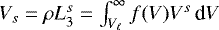 is the volume occupied by solid s per volume of stellar atmosphere and
 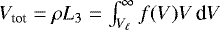 is the total solid volume per volume of stellar atmosphere.
The code is available at https://github.com/pw31/Diffusion.
All Tables
MRN astronomical silicate dust extinction opacities for selected wavelengths λ, see text for references.
All Figures
|
Fig. 1 Gas diffusion coefficient Dgas (Eq. (19)) in the new DIFFUDRIFT model for a brown dwarf atmosphere model with Teff = 1800 K, log g =3 [cm s−2] and solar abundances. The grey line shows the inverse mixing timescale τmix as assumed in the previous DRIFT model. τmix is calculated according to Eq. (9) in Woitke & Helling (2004). Both quantities are computed for β = β′ = 1, and both y-axes show exactly eight orders of magnitude. |
| In the text | |
|
Fig. 2 Operator splitting calling sequence. Sett = gravitational settling, Diff = diffusion, CF = cloud formation (nucleation, growth and evaporation), and OP = output. 1/2 means half a time step, and 1 is a full time step. |
| In the text | |
|
Fig. 3 Comparison of cloud formation models for Teff = 1800 K, log g =3, metallicity Z = 1, and β = β′ = 1. The previous DRIFT model is shown by the thick grey lines. Two DIFFUDRIFT models are overplotted assuming pure gas diffusion (dashed lines) and gas + particle diffusion (black solid lines). dust/gas = ρdL3 is the dust-to-gas mass ratio, nd = ρL0 the number density of cloud particles, |
| In the text | |
|
Fig. 4 Effect of our assumptions on the mixing processes in the atmosphere on the resulting gas element abundances, in models with the same parameters as in Fig. 3. Upper plot:
|
| In the text | |
|
Fig. 5 Material volume composition of the cloud particles |
| In the text | |
|
Fig. 6 Column densities [g cm−2] of different condensates in the atmosphere for a sequence of models with decreasing Teff but constant logg = 3 and β′ = 1. A value of 10−3 g cm−2 roughly corresponds to an optical depth of one at a wavelength of λ = 1 μm (see Appendix E). |
| In the text | |
|
Fig. 7 Sequence of cloud forming models with decreasing Teff at constant logg = 3 and mixing power-law index β′ = 1. Top row: gastemperature T and diffusioncoefficient Dgas as a functionof pressure (both assumed). Middle row: resulting dust-to-gas mass ratio and element abundance of silicon in the gas phase ɛSi. Lower row: resulting nucleation rates J⋆ and mean particle sizes |
| In the text | |
|
Fig. 8 Concentration of condensed species in a model with Teff = 1300 K,
log g =3, and β′ = 1, showing a secondary cloud layer almost entirely made of di-sodium sulfide Na2 S[s]. |
| In the text | |
|
Fig. A.1 Test problem with fixed concentrations on the left and right boundaries (ɛ = 0). The thin black lines overplot the analytic solution ɛ(z, t) = exp(−ωt)sin(kz) with k = π and ω = Dk2. |
| In the text | |
|
Fig. A.2 Diffusive evolution of an initial δ peak with analytic solution overplotted. The analytic solution is |
| In the text | |
|
Fig. A.3 Testing the model convergence for different initial conditions: gas element abundances ɛk as a functionof pressure p in two cloud formation models with different initial conditions, “empty” (left) and “full” (right), see text for further explanations. Panels from top to bottom: respective results after t = 0, t = 10 days, and t = 8000 days. |
| In the text | |
Current usage metrics show cumulative count of Article Views (full-text article views including HTML views, PDF and ePub downloads, according to the available data) and Abstracts Views on Vision4Press platform.
Data correspond to usage on the plateform after 2015. The current usage metrics is available 48-96 hours after online publication and is updated daily on week days.
Initial download of the metrics may take a while.