| Issue |
A&A
Volume 633, January 2020
|
|
|---|---|---|
| Article Number | A135 | |
| Number of page(s) | 15 | |
| Section | Stellar structure and evolution | |
| DOI | https://doi.org/10.1051/0004-6361/201936831 | |
| Published online | 22 January 2020 | |
Properties of carbon stars in the solar neighbourhood based on Gaia DR2 astrometry⋆
1
Dpto. Física Teórica y del Cosmos, Universidad de Granada, 18071 Granada, Spain
e-mail: This email address is being protected from spambots. You need JavaScript enabled to view it.
2
Université Côte d’Azur, Observatoire de la Côte d’Azur, CNRS, Laboratoire Lagrange, 06304 Nice Cedex 4, France
3
Istituto Nazionale di Astrofisica – Osservatorio Astronomico d’Abruzzo, Via Maggini snc, 64100 Teramo, Italy
4
INFN – Sezione di Perugia, Via A. Pascoli, Perugia, Italy
Received:
2
October
2019
Accepted:
14
November
2019
Abstract
Context. Stars evolving along the asymptotic giant branch (AGB) can become carbon rich in the final part of their evolution. The detailed description of their spectra has led to the definition of several spectral types: N, SC, J, and R. To date, differences among them have been partially established only on the basis of their chemical properties.
Aims. An accurate determination of the luminosity function (LF) and kinematics together with their chemical properties is extremely important for testing the reliability of theoretical models and establishing on a solid basis the stellar population membership of the different carbon star types.
Methods. Using Gaia Data Release 2 (Gaia DR2) astrometry, we determine the LF and kinematic properties of a sample of 210 carbon stars with different spectral types in the solar neighbourhood with measured parallaxes better than 20%. Their spatial distribution and velocity components are also derived. Furthermore, the use of the infrared Wesenheit function allows us to identify the different spectral types in a Gaia-2MASS diagram.
Results. We find that the combined LF of N- and SC-type stars are consistent with a Gaussian distribution peaking at Mbol ∼ −5.2 mag. The resulting LF, however, shows two tails at lower and higher luminosities more extended than those previously found, indicating that AGB carbon stars with solar metallicity may reach Mbol ∼ −6.0 mag. This contrasts with the narrower LF derived in Galactic carbon Miras from previous studies. We find that J-type stars are about half a magnitude fainter on average than N- and SC-type stars, while R-hot stars are half a magnitude brighter than previously found, although fainter in any case by several magnitudes than other carbon types. Part of these differences are due to systematically lower parallaxes measured by Gaia DR2 with respect to HIPPARCOS values, in particular for sources with parallax ϖ < 1 mas. The Galactic spatial distribution and velocity components of the N-, SC-, and J-type stars are very similar, while about 30% of the R-hot stars in the sample are located at distances greater than ∼500 pc from the Galactic plane, and show a significant drift with respect to the local standard of rest.
Conclusions. The LF derived for N- and SC-type in the solar neighbourhood fully agrees with the expected luminosity of stars of 1.5−3 M⊙ on the AGB. On a theoretical basis, the existence of an extended low-luminosity tail would require a contribution of extrinsic low-mass carbon stars, while the high-luminosity tail would imply that stars with mass values up to ∼5 M⊙ may become carbon stars on the AGB. J-type stars differ significantly not only in their chemical composition with respect to the N- and SC-types, but also in their LF, which reinforces the idea that these carbon stars belong to a different type whose origin is still unknown. The derived luminosities of R-hot stars means that it is unlikely that these stars are in the red-clump, as previously claimed. On the other hand, the derived spatial distribution and kinematic properties, together with their metallicity values, indicate that most of the N-, SC-, and J-type stars belong to the thin disc population, while a significant fraction of R-hot stars show characteristics compatible with the thick disc.
Key words: stars: late-type / stars: carbon / techniques: photometric / astrometry
Table 1 is only available at the CDS via anonymous ftp to cdsarc.u-strasbg.fr (130.79.128.5) or via http://cdsarc.u-strasbg.fr/viz-bin/cat/J/A+A/633/A135
© ESO 2020
1. Introduction
After He exhaustion, low- and intermediate-mass stars (0.8 ≤ M/M⊙ ≤ 8) populate the giant branch in the Hertzsprung Russell diagram for a second time. Stars in this phase of stellar evolution are known as AGB stars. AGB stars are very important contributors (> 50%) to the mass ejected by all stars into the interstellar medium (ISM). Therefore, they play a significant role in the chemical evolution of galaxies (see e.g. Wallerstein et al. 1997). Furthermore, they trace intermediate-age stellar populations so that they can be used in studies of Galactic structure (e.g. Cole & Weinberg 2002; Renzini 2015; Capozzi et al. 2016; Javadi & van Loon 2020). All these research topics rely on an appropriate estimation of the stellar parameters, and in particular on the mass.
The most important chemical peculiarity of AGB stars is that many of them are carbon rich (i.e. they show an abundance ratio C/O > 1 in their atmosphere). Since the overwhelming majority of stars are born with C/O < 1, this carbon enrichment must result from an in situ process that pollutes the envelope with fresh carbon produced in the interior or, alternatively, from a transfer of carbon-rich material in a binary system. In the first case the stars are called intrinsic carbon stars, and in the second case extrinsic carbon stars. It is well established that quasi periodic shell 4He burning occurs during thermal pulses (TPs) on the AGB, inducing mixing episodes (the third dredge-up, TDU) that increase the atmospheric C-to-O ratio in these red giants (see e.g. Iben & Renzini 1983; Straniero et al. 2006; Karakas & Lattanzio 2014). This gives rise to the spectral sequence of M to MS to S to SC to C as C/O increases in the envelope along the AGB phase. This increase in C/O is accompanied, in general, by an increasing s-process overabundance. Thus, the MS, S, SC, and C stars are heavy element-rich AGB stars, which has been confirmed by many spectroscopic studies (see Smith & Lambert 1990; Busso et al. 1992; Lambert et al. 1995; Van Eck et al. 1998; Van Eck & Jorissen 1999; Abia & Wallerstein 1998; Abia et al. 2002, among many others). However, the mass range for the formation of an AGB carbon star is still rather controversial. This is mainly due to our limited modelling of the TDU episodes and to our poor knowledge of the mass-loss rate occurring during the AGB. Even so, there is an ample consensus that the lower mass limit for the formation of a carbon star at solar metallicity is ∼1.5 M⊙, and that this limit decreases with decreasing metallicity. The latter is due to the fact that metal-poor stars have less O in their envelopes (which means that it is easier for the C/O to be above unity) and to the fact that the efficiency of the TDU increases at low metallicity. The upper mass limit is, nevertheless, more uncertain. Theoretically, stars with M ≳ 3 − 4 M⊙ may burn hydrogen through the CNO by-cycle at the base of the convective envelope (known as hot bottom burning, HBB), avoiding the formation of an AGB carbon star and substantially altering the CNO isotopic ratios, lithium, and other light element abundances (e.g. F, Na) in the envelope. This depends on the actual mass and metallicity of the star. However, these findings are extremely dependent on the mixing treatment, and the mass-loss and thermonuclear reaction rates adopted in the stellar modelling (see Lattanzio 2003; Straniero et al. 2006; Karakas & Lattanzio 2014; Ventura et al. 2015, for detailed discussions). Unfortunately, very few observational studies of massive AGB stars exist to constrain theoretical models in this sense (McSaveney et al. 2007; García-Hernández et al. 2007; Abia et al. 2017a), not to mention the difficulty in the determination of accurate masses (luminosities) for these stars (see e.g. van Loon et al. 1997, 1999; Frost et al. 1998; Marigo et al. 1999; Zijlstra et al. 2006; Groenewegen et al. 2007; Pastorelli et al. 2019).
Until recently, our knowledge of the luminous red giant carbon stars was limited to their spectral types, inaccurate radial velocities, and some uncertain proper motions, but detailed descriptions of their spectra. The last of these included the identification of key molecules such as C2, CH, and CN in the visual and infrared wavelengths and the recognition that some had enhanced lines of heavy elements. There are several types of carbon stars classified spectroscopically, mainly depending on the intensity of the molecular bands mentioned above and their effective temperature (Keenan 1993; Barnbaum et al. 1996; Wallerstein & Knapp 1998). During the past few decades, quantitative abundance and isotopic ratio determination in carbon stars of all types has allowed us to differentiate among them, and has given us a better understanding of their nucleosynthetic histories (sometimes affected by binarity) and evolutionary status. Among the red giant carbon stars four spectral types can be distinguished1. In what follows we summarise their main properties; a more detailed and extended discussion can be found in Jura (1991), Barnbaum et al. (1996), Wallerstein et al. (1997), Wallerstein & Knapp (1998), Knapp et al. (2001), Bergeat et al. (2002), Abia et al. (2003), Zamora et al. (2009), and references therein.
The normal N-type (or just C) objects are the most numerous. They are cool (Teff < 3500 K) and luminous objects (∼104 L⊙). Their spectra are very crowded showing intense carbon-bearing molecular absorptions and, in particular, a strong flux depression at λ ≲ 4000 Å. By definition these stars show C/O > 1 (although not much higher than unity) and most of them are enhanced in s-elements and fluorine at near-solar metallicity ([Fe/H] ≈ 0.0)2. The observed carbon, s-element and fluorine enhancement are believed to be produced by the recurrent mixing into the envelope of material exposed to He-burning through the TDU episodes (i.e. they are intrinsic carbon stars). Due to their high luminosities, they can be easily identified in the galaxies of the Local Group (see e.g. Rowe et al. 2005; Boyer et al. 2013; Whitelock 2020).
The stars of SC-type are characterised mainly by a C/O ≈ 1, which makes their spectra less crowded by molecular absorptions allowing the identification of a plethora of atomic lines. In the classical picture, these stars should correspond to a very short period in the evolution along the AGB phase when the star is transformed from an M (MS, S) (with C/O < 1) into a genuine carbon star (N-type with C/O > 1) due to the TDU episodes. Their chemical properties are indistinguishable from those observed in the N-type (or in the S-type stars; see e.g. Van Eck et al. 1998; Neyskens et al. 2011), although there is a hint indicating that SC-type show higher 16O/17O than the N-type (Abia et al. 2017b). Since a high value of 16O/17O is a characteristic of the operation of HBB, if confirmed these stars may be intermediate mass (≳3 − 4 M⊙). They then might become C-rich at the very end of their lives because of the cessation of the HBB when their envelope mass has been significantly reduced by strong mass loss (see e.g. Karakas & Lattanzio 2014). Only a dozen or so of SC-type stars are identified in the Galaxy (Catchpole & Feast 1971), and a few of them are among the most Li-rich stars ever found (Abia et al. 1999)3.
The J-type carbon stars are easily recognised from the intensity of carbon-bearing molecular bands formed with 13C atoms; their main chemical property is their very low ratio of 12C/13C, close to the CNO-cycle equilibrium value (∼3.5). They show C/O values in a range similar to that found in the N-type, but a significant fraction (80%) are Li-enhanced. They do not show s-element or fluorine enhancements (Abia & Isern 2000; Abia et al. 2015). They are also solar metallicity stars. These chemical peculiarities clearly differ from those of N- and SC-type stars. Therefore, the location of J-type stars in the AGB spectral sequence above is far from clear. It has been suggested that the mass transfer scenario is at the origin of their carbon enhancement (i.e. they would be extrinsic carbon stars). In some of them, silicate emission has been detected in their infrared spectrum, which usually is associated with the presence of a circumbinary disc around a binary system (see e.g. Deroo et al. 2007). However, aside from the fact that no radial velocity variations have been detected yet in any of these stars, it is not clear how their Li enhancement can be explained in the mass transfer episode. Other scenarios have been proposed, such as the mixing of fresh carbon after a peculiar He-flash induced by a rapidly rotating core (e.g. Mengel & Gross 1976), or the re-accretion of carbon-rich nova ejecta on main-sequence companions to low-mass carbon-oxygen white dwarfs (Sengupta et al. 2013). Although their origin is unknown, they represent about 15% of all Galactic carbon stars and a similar fracion has also been identified in Local Group galaxies (Morgan et al. 2003).
Finally, R-hot (or early) carbon stars are the warmest (Teff ≳ 3800 K) objects and are easily identified spectroscopically because of their less crowed spectra and weaker molecular absorptions compared to the rest of the carbon star types4. These stars do not have a particular chemical property, with one exception: they do not show s-element enhancements. It is well established that these stars are much fainter than the rest of the carbon types. Using HIPPARCOS parallaxes, Knapp et al. (2001) placed them in the red-clump region on the H-R diagram with a mean luminosity MK ≈ −2.0 mag, which is compatible with core He-burning stars. Furthermore, most of these early R-type stars are non-variable, and their infrared photometric properties show that they are not undergoing significant mass loss, as opposed to the other three spectral types. No radial velocity variations have been detected in the R-hot stars (McClure 1984), which would eliminate the mass transfer scenario as an explanation of their carbon enhancement. The favoured hypothesis so far is that the carbon produced during the He-flash is mixed in some way to the surface. However, the general conclusion is that hydrostatic models do not produce mixing at the He-flash, thus other scenarios have been explored. An anomalous He-flash after a red giant star’s merging has been suggested, but there are many difficulties in using this scenario to explain the observed chemical properties (Izzard et al. 2007; Piersanti et al. 2010). Recently, Zhang & Jeffery (2013) found that a high-mass helium white dwarf subducted into a low-core-mass red giant could produce a R-hot star with the observed chemical properties. Furthermore, in this scenario J-type stars may represent a short and luminous stage in the evolution of a R-hot star. Nevertheless, considering that R-hot stars represent ∼30% (Bergeat et al. 2002) of all luminous red giant carbon stars, we need to show that this scenario can account for the observed statistics.
As follows from the above discussion, similarities and differences among the different spectral types have been made mainly on the basis of their observed chemical pattern. However, the conclusions deduced from these abundance studies are frequently limited by the uncertain determination of the mass, luminosity, and kinematics properties of the stars. The Gaia all-sky survey is changing this situation by providing astrometric data with an unprecedented accuracy of all Galactic stellar populations. In the Gaia DR2 release (Gaia Collaboration 2018), the first Gaia catalogue of long-period variables (LPVs) with G-band variability amplitudes larger than 0.2 mag has been published (Mowlavi et al. 2018). It contains 151 761 candidates, among them thousands of luminous carbon stars of variable types: Mira, irregular, and semi-regular. The aim of the present study is to use the Gaia DR2 information available for a sample of already known red giant carbon stars of different spectral types located in the solar vicinity to derive their luminosity and kinematic properties. These quantities are discussed together with their chemical characteristics to obtain a global picture of the different carbon star types and to discern between the various types in terms of luminosities, masses, evolutionary stages, and kinematics.
The structure of the paper is as follows. In Sect. 2 we describe the adopted sample of carbon stars and study their spatial distribution in the solar neighbourhood. In Sect. 3 we describe the derivation of the luminosity distribution of the sample and its implications on the possible masses and evolutionary status of the sample stars. In Sect. 4 we derive their kinematic properties. In Sect. 5 we show how the combination of Gaia and infrared photometry allows the identification of the different spectral types of carbon stars in the Gaia-2MASS diagram, as has been recently done for the LPV in the Large Magellanic Cloud. Finally, in Sect. 6 we summarise the main results of this study.
2. Stellar sample and spatial distribution
Different samples of Galactic AGB stars, selected on the basis of their infrared properties, can be found in the literature, for instance Claussen et al. (1987), Willems (1988), Jura & Kleinmann (1989), and Groenewegen et al. (1992). Among these surveys the most extensive is that by Claussen et al. (1987), which focuses exclusively on luminous carbon stars. This survey was used by Boffin et al. (1993) and Abia et al. (1993) to study the frequency of the Li enrichment among Galactic carbon stars. Furthermore, there is valuable information on the chemical properties of many objects, obtained from high-resolution spectroscopic studies (see references in Sect. 1). We decided, therefore, to base our study on the survey by Claussen et al. (1987). This sample was drawn from the Two Micron Sky Survey (Neugebauer & Leighton 1969), which is expected to be statistically complete for sources brighter than K ∼ +3.0 mag over the region −33° < δ < +81°. This sample contains 214 Galactic carbon stars to which we have added some additional carbon stars with already well-determined photospheric characteristics and, in particular, chemical properties (e.g. Lambert et al. 1986; Abia et al. 1993, 2002, 2015; Ohnaka & Tsuji 1996; Abia & Wallerstein 1998; Abia & Isern 2000; Vanture et al. 2007, and references therein). Spectral types were taken directly from the SIMBAD5 database, although a few stars were re-classified according to the more detailed spectroscopic studies mentioned above. This initial sample was then filtered considering the quality of their Gaia DR2 parallaxes (Gaia Collaboration 2018). For the present study, only stars with good-quality DR2 parallaxes (ϖ) were selected, that is, those matching the condition ϵ(ϖ)/ϖ ≤ 0.20. We note, however, that the overwhelming majority of the stars (∼85%) in our sample have Gaia DR2 parallax uncertainty ≤10%. This condition ensures that the distance adopted from Bailer-Jones et al. (2018) is close to the inverse of the parallax, and therefore has little dependence on the adopted prior. Applying the above parallax uncertainty criterion, our final sample consists of 10 stars of SC-type, 22 of J-type, and 143 of N-type; 80% of them have a parallax uncertainty smaller than 10%. Furthermore, for comparison purposes, we added 10 O-rich AGB stars of M-type and 35 R-hot type carbon stars fulfilling the above-mentioned parallax criterion, the latter were selected from the magnitude-limited study of Knapp et al. (2001); some of them were analysed chemically by Dominy (1984) and Zamora et al. (2009). We note that several of the R-hot stars included in the study of Knapp et al. (2001) were discarded here because they have been re-classified as CH, Ba, and/or CEMP stars or because their spectral type appears rather doubtful in the literature6. The few O-rich AGB stars were taken from the study of García-Hernández et al. (2007) and are expected to be intermediate-mass stars probably undergoing HBB because of their strong Li absorption at λ6078 Å (see below).
Except for the R-hot type, the vast majority of the stars in our sample are known or suspected variables. We have 28 Mira variables among the C- and O-rich stars, the others being irregular or semi-irregular variables. Only a couple of R-hot stars in the sample, however, are classified as variables of R CrB type. Finally, from the chemical studies mentioned above, the overwhelming majority of the selected stars have near-solar metallicity ([Fe/H] ∼ 0.0 ± 0.3). As a consequence and unless explicitly mentioned, we assume throughout this paper a solar metallicity for all of the stars in our sample.
The sample stars are listed in Table 1 (Col. 1), adopting preferentially their variable star designation (from Samus et al. 2004, hereafter GCVS) or, if not available, the most commonly used name in the literature (checked with the SIMBAD database). For the R-hot stars, we used instead their HIPPARCOS catalogue identification. For all the sample stars, we then searched for their Gaia DR2 identification in the Gaia database web facility using the adopted target names of Table 1 and recovered all the Gaia astrometric information available. We adopted the distance estimates and associated uncertainties of Bailer-Jones et al. (2018) for all of the sample. For the line-of-sight velocities, we first adopted the values given in Menzies et al. (2006) for 13 stars that rely on CO millimetre lines measurements. These estimations are more accurate than classical ones from near-infrared (NIR) or optical spectral lines. Typical uncertainties reported in this work are of a few km s−1. For the other stars, we first retrieved from CDS/SIMBAD all the available bibliographic heliocentric radial velocity measurements, Vrad. When possible, we favoured the values reported in the Pulkovo Compilation of Radial Velocities (Gontcharov 2006), which have a median accuracy of about ±1 km s−1. If not present in this catalogue either, we adopted the Vrad measurement of the most recent reference found in SIMBAD. Finally, for the few stars without any reported Vrad in the above references, we adopted the Gaia DR2 Vrad (Katz et al. 2019). We decided not to adopt a priori the Gaia DR2 Vrad for all our sample stars since the Gaia radial velocity spectral domain is not optimal for deriving Vrad in cool carbon-rich stars. Their spectra are crowded by molecular absorptions and the IR CaII triplet is usually not easily visible in such stars (see e.g. Barnbaum et al. 1996). Moreover, as far as we know, the Gaia DR2 pipeline for Vrad derivation is not optimised for analysing (not known a priori) carbon-enhanced spectra. This, however, does not concern the R-hot stars, for which, due to their warmer effective temperature (Teff ≥ 3800 K), the IR CaII triplet can be easily identified and is thus useful for radial velocity determinations. For these stars, we have taken directly the Gaia DR2 Vrad values (Katz et al. 2019).
The distances and Vrad values finally adopted in this study are reported in Table 1. These are the main parameters from which the luminosities and kinematic properties are derived. To check the quality of the Gaia DR2 astrometric data for our sample stars, we have looked at their renormalised unit weight error (RUWE). This error coefficient can be used to identify possible non-single stars and/or possible problematic cases of the astrometric solution (see Gaia DR2 documentation, Sect. 14.1.2 and Lindegren 2018). Typically, according to the Gaia documentation, poor astrometric fits have a RUWE parameter larger than ∼1.4. We find that 70%, 90%, and 94% of our sample stars have a RUWE factor less than 1.0, 1.2, and 1.4, respectively. We have also checked the correlations between the RUWE factor and the parallaxes or the proper motions. No correlation is seen with the parallaxes; however, a slight increase in the proper-motion error for the stars having RUWE greater than 1.2 is seen, increasing from ∼0.2 mas yr−1 to ∼0.4 mas yr−1. We note, however, that these errors still remain small (and affect less than 10% of the stars). We are therefore confident in the astrometric data adopted in this study. Nevertheless, we note here that the Gaia DR2 procedure to compute the parallax contains colour- and magnitude-dependent terms. For the HIPPARCOS survey, Pourbaix et al. (2003) and Platais et al. (2003) advocated the importance of the colour bias on the astrometry, particularly for very red objects. Because most stars in our sample show large colour variations within a cycle (they are variable stars), chromaticity corrections must be applied to each epoch data. On the contrary, Gaia DR2 parallaxes are determined assuming a constant mean colour and magnitude for each source (Lindegren et al. 2018). Another phenomenon that may affect the parallax measurement of late-type stars, in particular its accuracy, is the possible displacement of the photometric centroid (photocentre) of the star with respect to the projected barycentre due to surface brightness asymmetries (e.g. due to granulation- or convection-related surface variability). Ludwig (2006) has shown that these effects may be considerable in red super giants. Recently Chiavassa et al. (2018) studied the limits in astrometric accuracy of Gaia induced by these surface brightness asymmetries on the basis of radiative hydrodynamic simulations of AGB stars. They conclude that the displacement can be a non-negligible fraction of the star radius R (5 − 10% of the corresponding stellar radius), accounting for a substantial part of the parallax error. The above issues may affect the measured parallaxes as well as their accuracy7. We cannot exclude, therefore, that the parallax for some of our selected stars could be incorrectly evaluated in Gaia DR2. Our conclusion, nevertheless, is that our results should not be affected significantly by possible astrometric problems since the RUWE parameters of our sample are in average quite small (median = 0.94 and mean = 1.1). Obviously the increase in the parallax estimates over one-year cycles expected in Gaia DR3 would reduce the error on the mean parallax.
Figure 1 shows the comparison between HIPPARCOS (van Leeuwen 2007; Knapp et al. 2001, for R-type stars) and Gaia DR2 parallaxes for 139 stars in common with our sample. From this figure, it is evident that HIPPARCOS parallaxes tend to be much larger than Gaia DR2 ones, particularly for ϖ ≲ 1 mas. For ϖ ≳ 1 mas, Gaia DR2 and HIPPARCOS parallaxes appear to be symmetrically distributed around the equal-parallax line. Globally, we find a mean difference of Δϖ = 0.56 ± 1.70, in the sense HIPPARCOS minus Gaia DR2. Obviously this difference has a significant impact on the luminosities derived for our stars compared to those based on HIPPARCOS parallaxes (see Sect. 3).
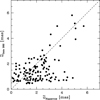 |
Fig. 1. Comparison between the HIPPARCOS and the Gaia DR2 parallaxes for 139 stars in common with our sample of Galactic carbon stars. Typical parallax errors are of the order of 50% (or even larger) for HIPPARCOS and smaller than 15% for Gaia. Error bars are omitted in the plot for clarity. The HIPPARCOS parallaxes are systematically larger for sources with Gaia ϖ ≲ 1 mas. See text for details. |
Figure 2 shows the location of the sample stars onto and above or below the Galactic plane (see also Table 1). Their Cartesian coordinates have been directly derived from the Gaia DR2 sky coordinates and adopted distances. The uncertainties on the individual X, Y, Z, and R positions are estimated as the dispersion of these values for each star, over 500 Monte Carlo realisations of the Bailer-Jones et al. (2018) line-of-sight distances8, assuming no uncertainty on the right ascension or declination sky coordinates (see also Sect. 4). Median uncertainties are ±12, 16, 13, and 13 pc for X, Y, Z, and R, respectively.
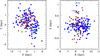 |
Fig. 2. Left: location of the sample carbon stars of different spectral types on the Galactic plane. The Sun is placed at (X, Y) = (0, 0). Stars shown are N-type (blue); J-type (red); SC-type (green), and R-hot type (brown). Right: distribution above or below the Galactic plane vs. the Galactocentric distance. The Sun is at R = 8.34 kpc. The typical uncertainty in the (X, Y, Z) coordinates is ±20 pc, and ±50 pc for the Galactocentric distance. Two N-type stars with peculiar locations above the Galactic plane are labelled (see text). |
From the left panel of this figure it appears that the spatial distribution of the N-, J-, and SC-type stars (in blue, red, and green, respectively) is fairly uniform within a radius of ∼1.5 kpc from the Sun, in the region of the sky observed by the Two Micron Sky Survey. In fact, the apparent lack of these spectral type sources in the region with X < 0 and Y < 0 is simply due to the incomplete coverage of this survey: the southern declination limit being −33°. A few N-type stars, however, seem to be located beyond this radius. Furthermore, for these spectral types, it can also be appreciated that there is no specific concentration of carbon stars in either direction. This agrees with the conclusions of Claussen et al. (1987). In contrast, our sample of R-hot stars (brown circles in Fig. 2) seem less homogeneously distributed around the Sun with, apparently, an overdensity around it. The left panel of Fig. 2 shows that carbon stars of N-, J-, and SC-types are rather concentrated towards the Galactic plane with no appreciable difference between the different spectral types in the height from the plane. Claussen et al. (1987) argued that the present sample of carbon stars should be complete within 1.5 kpc from the Sun on the hypothesis that all the carbon stars have an absolute magnitude MK = −8.1 mag (we confirm this hypothesis here, see below) and considering that the limit of the Two Micron Sky Survey in K is ∼ + 3.0 mag. A comparison with the number of carbon stars detected in other similar surveys shows that this expectation is fulfilled (for details, see Claussen et al. 1987). On this basis, a crude fit to the z-coordinate distribution, excluding the R-hot stars, with an exponential function results in a scale height of zo = 180 ± 20 pc. Considering only the N-type stars would slightly change this value. We note that only two N-type stars, V CrB and RU Vir, are located well above the Galactic plane. We show in the following sections that also their peculiar kinematics could point towards a possible thick disc (or halo) membership or even an extragalactic origin. Ignoring these two stars, the measured scale height agrees well with the range 150−250 pc estimated by Claussen et al. (1987). This scale height can then be used to estimate the typical mass of carbon star progenitors by using tabulations for the scale heights of main-sequence stars as a function of spectral class as, for example, in Miller & Scalo (1979). This study showed that stars with a mean scale height in the range 160−190 pc have a mass between 1.5 and 1.8 M⊙. These values are fully consistent with theoretical determinations of the typical mass for an AGB carbon star (see e.g. Straniero et al. 2006; Karakas & Lattanzio 2014). Contrary to N-, J-, and SC-type stars, it is also evident from Fig. 2 that the R-hot carbon stars reach larger distances from the Galactic plane than the other carbon-type stars. In fact, they are distributed quite uniformly in |z| within 0 ≤ |z| ≤ 1 kpc, the average value being |z| = 510 ± 300 pc; only one star HIP 48329 is located at |z| > 1 kpc (not shown in Fig. 2 for clarity, see Table 1). Since the Galactic stellar population scale height is believed to be a function of age (mass) (see e.g. Dove & Thronson 1993), this implies that R-hot stars are likely older and have lower masses than the N-, J-, and SC-type stars. This also confirms the conclusion already reached in previous studies (Wallerstein & Knapp 1998; Knapp et al. 2001; Izzard et al. 2007, 2008; Zamora et al. 2009).
3. Gaia DR2 luminosities of carbon stars
The determination of the bolometric correction (BC) for cool giants is still an open issue (see e.g. Bessell & Wood 1984; Bessell et al. 1998; Montegriffo et al. 1998; Costa & Frogel 1996; Houdashelt et al. 2000, among many others). This is particularly challenging for AGB stars whose stellar flux is affected by millions of molecular absorptions. Furthermore, the formation of circumstellar shells around these evolved stars may absorb or scatter part of their stellar flux that is redistributed towards the mid- and far-infrared ranges. There is still not adequate description for such complex processes. It is therefore not surprising that in the extant literature the BCs adopted for AGB stars may differ by up to 0.5 mag. In the present work we adopt the empirical BCK versus (J − K) relation for C-stars obtained by Kerschbaum et al. (2010), which is based on a critical revision of the available studies. For (J − K) between 1.0 and 4.4, the maximum standard deviation of this relation is 0.11 mag. We also use this BC relation for the R-hot stars, which typically show (J − K) colours slightly bluer (∼0.7 − 0.8 mag) than the range of validity of the Kerschbaum et al. (2010) calibration. We note, however, that other BCK versus (J − K) calibrations found in the literature for (J − K) < 1 values provide BCK corrections differing by less than 0.1 mag (e.g. Bessell & Wood 1984; Montegriffo et al. 1998) with respect to that we adopt here. Finally, for the O-rich AGB stars in the present study (see Table 1), we also adopt the BCK versus (J − K) relation derived by Kerschbaum et al. (2010) for M stars.
Then, we retrieved the 2MASS J and Ks photometry (Cutri et al. 2003) from the SIMBAD database and corrected the values for the interstellar extinction according to the Galactic model of Arenou et al. (1992), using the Bailer-Jones et al. (2018) derived distances and the Gaia Galactic coordinates. For the reddening corrections, we used the relations AV = 0.114 ⋅ AK and AJ = 2.47 ⋅ AK. The corrected J and Ks magnitudes together with the calculated BCKs values are given in Table 1 for all the sample stars. The MKs and Mbol magnitudes were then derived from the distance modulus relation, and are also listed in Table 1. Uncertainties on MKs and Mbol are dominated by those on ϖ (distances). For the typical parallax uncertainty on our stars (≤10%, see Sect. 2) an error of ∼±0.20 mag on the absolute magnitudes is estimated. Obviously, for the few stars in the sample with parallax uncertainty within 10 − 20%, the error would be larger. We therefore adopted ±0.25 mag as a typical error for MKs and Mbol in the full sample of stars. The corresponding bolometric luminosity distributions or luminosity functions (LFs) obtained for all the carbon star types in our sample are shown in Fig. 3. Several remarks can be made.
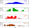 |
Fig. 3. Luminosity distributions derived in this study for the different spectral types of Galactic carbon stars. The bin size is 0.25 mag. The range of luminosities is different for the R-hot type stars, which are fainter. |
First, the LF of the N-type stars peaks at Mbol ∼ −5.2 mag, with extended tails towards lower and higher luminosities. A Kolmogorov–Smirnov (KS) test says that the distribution is consistent with a normal one when p = 0.6. The average luminosity of our selected N-type stars is ⟨Mbol⟩ =carbon stars. Their average magnitudes − 5.09 ± 0.58 mag. Within the quoted uncertainties, this average luminosity (∼104 L⊙) agrees with that found by similar studies of Galactic and LMC C-stars (e.g. Guandalini & Cristallo 2013; Gullieuszik et al. 2012) and with the theoretical expectations for stars with a ∼0.6 M⊙ He-core mass (Paczyński 1971). This occurrence confirms previous findings that the majority of the N-type carbon stars have an initial mass 2 ± 0.5 M⊙. However, unlike previous Galactic studies, we find a significant number of bright N-type stars (Mbol ≲ −5.8 mag), although none above the classical limit for AGB stars, Mbol = −7.1 mag9. In principle, this high-luminosity tail of the LF should be populated by AGB stars with higher core masses, and hence with higher initial mass (M > 3 M⊙). We note that stars with 3 < M/M⊙ < 5 will be very luminous objects in the AGB phase and will still become C-stars, but owing to the greater envelope dilution of the dredged up material, the time spent in the C-rich phase is quite short, and thus their contribution to the LF would be low. Moreover, in stars with mass M > 5 M⊙ the occurrence of the HBB prevents the formation of a C-rich envelope (see e.g. Karakas & Lattanzio 2014) and the stars may exceed the AGB luminosity limit. A more quantitative analysis of the LF tails, both at low and high luminosity, is illustrated in the next section. The derived average absolute K magnitude, ⟨MKs⟩ = − 8.16 ± 0.50, agrees closely with the values found in the NIR photographic surveys of the Magellanic Clouds (e.g. Frogel et al. 1980) and the Galaxy (Schechter et al. 1987), although we find a larger dispersion. Nevertheless, this dispersion in MK is compatible with the typical range in Teff (2500−3500 K) deduced for N-type stars (e.g. Bergeat et al. 2001).
Second, the LF of SC-type stars is rather similar to that of the N-type. This figure, together with the scarce number of SC-type carbon stars identified to date, is compatible with the hypothesis that the SC-type represents a short transition phase (C/O ≈ 1) between the O-rich (C/O < 1) and the C-rich (C/O > 1) AGB phases. Moreover, the very similar chemical composition shared by N- and SC-type carbon stars (Abia & Wallerstein 1998; Abia et al. 2002, 2019), as well as their similar location above or below the Galactic plane (see Sect. 2), support the conclusion that both types of carbon stars originate from similar progenitors. In any case, the identification and analysis of more SC-type stars is needed to reach a definite conclusion. In the following, we tentatively assume that SC- and N-type belong to the same stellar population.
Third, J-type stars show a significantly dimmer LF compared to that of N-type carbon stars. Their average magnitudes are ⟨Mbol⟩ = − 4.66 ± 0.40 mag and ⟨MKs⟩ = − 7.70 ± 0.40 mag. Although these luminosites are within the AGB range, a non-negligible fraction of the J-type stars are fainter than Mbol = −4.5 mag, which represents the threshold for the occurrence of TDU episodes (see e.g. Straniero et al. 2003; Cristallo et al. 2011). Therefore, J-type stars differentiate from N-type stars not only in their chemistry, but also in their luminosity, which reinforces the idea that these stars have (as their carbon enhancement) a different origin. This is the first time that this conclusion has been reached on the basis of a homogeneous luminosity study.
Finally, as already noted, R-hot carbon stars show a much dimmer LF than that of the AGB stars; we find ⟨Mbol⟩ = − 0.10 ± 0.80 mag and ⟨MKs⟩ = − 2.54 ± 1.03 mag, the latter being about half a magnitude brighter than that previously determined by Knapp et al. (2001). We note that the main reason of this discrepancy is the systematic difference between the Gaia DR2 and HIPPARCOS parallaxes (see Sect. 2). This occurrence is at odds with their suggestion that these objects are He-burning red-clump stars. The luminosity of the red clump is expected for solar metallicity stars at ⟨MKs⟩∼ − 1.6 ± 0.3 mag (e.g. Alves 2000; Castellani et al. 2000; Salaris & Girardi 2002). On the contrary, our derived luminosities put the R-hot stars in the upper part of the red giant branch (RGB). Therefore, the hypothesis that the carbon enhancement in a significant fraction of the R-hot is produced by the C dredge-up powered by the violent off-centre He ignition (He flash) in the degenerate core of low-mass stars must be discarded. Furthermore, comparing the range of Mbol derived here for both the R-hot and the J-type stars, it also seems very unlikely that the latter type represents a luminous phase of R-hot stars, in the hypothesis that they are formed from a high-mass helium white dwarf subducted into a low-core-mass red giant (Zhang & Jeffery 2013). The possibility that J-type stars are the descendants of the R-hot ones in a more advanced evolutionary stage seems to be discarded.
In Fig. 4, we compare the LF derived in the present study (N- and SC-type carbon stars) with the LF obtained for AGB carbon stars in three representative similar studies. We exclude the J-type and the R-hot stars since, as previously shown, these carbon stars probably have a different origin. In particular, we compare our derived LF with those of (i) the VISTA survey of AGB stars in the Large Magellanic Cloud (Gullieuszik et al. 2012, 93 stars, black-dotted line)10. (ii) the sample of Galactic carbon stars by Guandalini & Cristallo (2013) (102 stars, red-dotted line), and (iii) the sample of Galactic Mira carbon stars by Whitelock et al. (2006) (145 stars, green-dashed line).
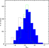 |
Fig. 4. Derived LF distribution of the present study (blue histogram, excluding J- and R-hot-type stars), compared to those obtained by Gullieuszik et al. (2012) (black dotted line) in the VMC survey of carbon stars, Guandalini & Cristallo (2013) (red dotted line) in Galactic AGB carbon stars, and Whitelock et al. (2006) in Galactic Mira carbon stars (green dashed line). The LFs of these studies have been re-binned with a 0.25 mag step for better comparison. |
Globally, the comparison with the Guandalini & Cristallo (2013) and Gullieuszik et al. (2012) LFs reveals that they appear ∼0.25 mag dimmer than our LFs. In the case of the Gullieuszik et al. (2012) LF and, since their BCK values are very similar to ours, we ascribe this difference to the lower average metallicity of the carbon stars in the Large Magellanic Cloud. At lower metallicity, owing to the lower O abundance in the envelope, the C-rich phase (C/O > 1) is more rapidly attained (i.e. at fainter luminosity) and lasts for a longer time. On the other hand, the differences with Guandalini & Cristallo (2013) can be explained mainly by the shorter distances derived by these authors compared to those we adopted: the average distance difference for the 21 stars in common is 210 pc, in the sense of the Guandalini & Cristallo (2013) values minus the present study’s values, with a significant dispersion (±240 pc). Actually, these authors adopted mainly HIPPARCOS parallaxes in their study. We recall that the HIPPARCOS parallaxes tend to be larger than those of Gaia DR2 for carbon stars (see Sect. 2). Differences in the adopted BC probably play a role as well: Guandalini & Cristallo (2013) used a BCK versus Ks − [12.5] relation, where [12.5] is the stellar flux at 12.5 μm. In general, we derived larger BCK than Guandalini & Cristallo (2013) for the stars in common, which may be partially compensated by the extinction corrections not considered by these authors. This shift towards weaker Mbol is not seen in the LF derived by Whitelock et al. (2006) for Galactic carbon Miras (green dashed line in Fig. 4), which peaks at the same Mbol ∼ −5.2 mag as ours. We recall that these authors derived their luminosities and distances on the basis of the period-luminosity relation found in the Miras of the LMC corrected by the Galactic zero point (Feast et al. 2006). Their BCs for the K-magnitudes were calculated from a relation with various infrared colours. In the particular case of the (J − Ks) relation, BC may differ by up to 0.3 mag with respect to the relation adopted here for the reddest objects (i.e. for (J − Ks) > 2 mag). For nine stars in common with these authors, we find a mean difference in the distance of 120 pc, in the sense of the Whitelock et al. (2006) values minus this study’s values, also with a significant dispersion (±250 pc). In any case, from Fig. 4 it can be appreciated that their LF is very narrow around the luminosity peak, as opposed to the other LFs shown in this figure. Moreover, their LF does not show any extended tails at low and high luminosity, contrary to what we clearly find. This difference indicates that carbon Miras may represent a distinct stellar population among the AGB carbon stars. We come back to this issue in the next section.
In Fig. 5 we compare our new derived LF distribution with its theoretical counterpart. Details about the derivation of such a theoretical distribution can be found in Guandalini & Cristallo (2013) (see also Cristallo et al. 2015). Here, we recall the basic concepts only.
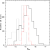 |
Fig. 5. Derived LF for our full sample of Galactic AGB carbon stars (solid black line, excluding J-type and R-hot stars) compared with the theoretical LFs described in Sect. 3 (red dashed histogram), and with the LF expected for a typical model of an extrinsic C-star (black dotted line; see text). The theoretical LFs are normalised such that the peak of a LF matches the peak of the corresponding observations. |
We extract the luminosities from our AGB models, sampling the C-rich phase with the same magnitude bins as the observational LF. We assign weights proportional to the time spent by the model in each magnitude bin. Then we populate our distribution by simulating a simple disc evolution with a Salpeter initial mass function (IMF) and a metallicity distribution from Cescutti & Molaro (2019). A linearly decreasing star formation rate is considered. The contribution of each star to the LF is a function of the time spent in the C-rich phase. We consider all stars attaining the C-rich regime (from 1.0 M⊙ to 6.0 M⊙, depending on the initial metallicity of the model). It must be noted that in the construction of the theoretical LF we consider the full evolutionary tracks of all the C-star models. These tracks already include, in particular, the post-flash luminosity dip, and so no correction is needed to account for this phenomenon (see Iben & Renzini 1983; Stancliffe et al. 2005).
The resulting theoretical LF is shown in Fig. 5 (red dashed histogram). We note that this new theoretical LF is shifted to slightly lower bolometric magnitudes with respect to those presented by Guandalini & Cristallo (2013) (see Fig. 4, red dotted histogram). This is a consequence of the adoption of new bolometric corrections in the derivation of the mass-loss rate. The mass-loss prescription of the FRUITY11 models is illustrated in Straniero et al. (2006). It consists of a fit, in the mass-loss versus period plane, to a sample of Galactic O-rich and C-rich giants. The stellar period is calculated by means of the MK-period relation proposed by Whitelock et al. (2003), and MK is derived from the bolometric magnitude of the model and a BCK versus Teff relation. At variance with Straniero et al. (2006), here we adopt an updated fit of the BCK versus Teff relation. In particular, we consider the Teff data of O-rich red giants from Buzzoni et al. (2010), extended at lower Teff with a sample of N- and SC-type carbon stars from Abia & Wallerstein (1998) and Abia et al. (2002). Then, the bolometric corrections are obtained by means of the BCK versus (J − K) relation of Kerschbaum et al. (2010) (see above). The new and the previous relations are compared in Fig. 6. We note that for Teff < 3500 K, which correspond to the typical temperatures of the C-stars, the new bolometric corrections are lower, and hence the resulting MK is higher. This occurrence implies a reduction of the mass-loss rate and, in turn, an increase in the C-star lifetime. As shown in Fig. 7, in the case of the 2 M⊙ model with Z = Z⊙, the duration of the C-rich phase increases (+84%), and the C/O ratio attains higher values (+18%). The new models experience a larger number of thermal pulses, and thus spend more time at the higher luminosities.
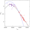 |
Fig. 6. Bolometric corrections as a function of the effective temperature. Data are from Buzzoni et al. (2010) (red squares) and this study (magenta circles). The new fit (black line) is compared with the one adopted by Straniero et al. (2006) (blue line). See text for details. |
The peak of the present theoretical LF is in good agreement with the observed one. It is important to note that intermediate-mass models (M > 4 M⊙) show a greater sensitivity to the new mass-loss rate, even if in our theoretical framework they rarely attain the C-rich stage (the O-rich TP-AGB phase of a 5 M⊙ model with Z = Z⊙ lasts 34% longer and the C/O ratio increases by 55%; see right panels of Fig. 7).
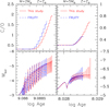 |
Fig. 7. Evolution of the C/O ratio (upper panels) and surface luminosity (lower panels) for models calculated with different mass-loss laws. See text for details. |
In spite of the good match of the central part of the LF, the theoretical prediction fails to reproduce both the low- and the high-luminosity tails of the observed LF. Interestingly, our theoretical LF agrees remarkably well with the LF of Galactic Mira carbon stars (green dashed histogram in Fig. 4). We suspect that this feature is a direct consequence of the fact that our mass-loss rate is calibrated on a Mira MK-period relation (Whitelock et al. 2003). Different mass-loss prescription could be more appropriate for the irregular and semi-regular pulsators, which are the overwhelming majority in our sample, possibly making the brightest tail appear. It this context, we noted that Stancliffe et al. (2005) obtained a LF with an extended high-luminosity tail by adopting the Vassiliadis & Wood (1993) mass-loss prescription. According to these authors, this prescription causes significant mass loss only when the estimated pulsation period exceeds 500 days, while a negligible mass loss is obtained during the major part of the AGB evolution. As a result, the carbon star phase is more easily attained in the more massive models, those populating the high-luminosity tails of the LF. In any case, the HBB should be inefficient in these stars, at least for those with mass M ≲ 5 M⊙, otherwise a C/O ratio well below unity would be maintained within the envelope. In other words, the observed existence of C-stars with −6.5 < Mbol < −5.5 severely constrains the occurrence of the HBB in intermediate-mass AGB stars12.
The low-luminosity tail is likely due to the contamination of our sample with extrinsic C-stars (i.e. stars that inherited their carbon enhancement from an already extinct carbon-rich AGB companion). Those extrinsic stars would approach the AGB phase already with C/O > 1 or very close to unity. Having lower core masses, they would show lower luminosities13. This idea was already suggested by Izzard & Tout (2004) to explain the low-luminosity tail of carbon stars in the SMC. On this same basis, we ran an exploratory case by accreting material with C/O > 1 on a 0.7 M⊙ main-sequence star from a more massive (3 M⊙) AGB companion. After the accretion episode, the mass attained by the secondary star is 1.0 M⊙. In Fig. 5 we show the luminosity distribution of this model (dotted black curve), using as weight the time spent in each luminosity bin. As can be seen, the low-luminosity tail of the observed LF could be easily matched under the assumption that a fraction of these accreting stars become C-rich.
4. Kinematics
Many studies prior to Gaia have shown that the major stellar structures identified in our Galaxy–the thin and thick discs and the halo–have distinct kinematic and chemical properties at least in the solar neighbourhood (e.g. Gilmore et al. 1989; Wyse & Gilmore 1995; Freeman & Bland-Hawthorn 2002; Bensby et al. 2003; Kordopatis et al. 2011; Ivezić et al. 2012; Recio-Blanco et al. 2014; Wojno et al. 2016). Therefore, the accurate kinematic properties of our sample stars, thanks to the Gaia DR2 astrometric data, provide an additional and valuable piece of information to fully characterise the stellar population of the different types of carbon stars.
To compute the Galactocentric positions and velocities, we used the line-of-sight distance estimates of Bailer-Jones et al. (2018), together with the RA, Dec, and proper motions of Gaia DR2 and our adopted line-of-sight velocities (Vrad). Furthermore, we assumed the following parameters: (R⊙, Z⊙) = (8.34, 0.025) kpc (Reid & Honma 2014), (U⊙, V⊙, W⊙) = (11.1, 12.24, 7.25) km s−1 (Schönrich 2012) and VLSR = 240 km s−1 (Reid & Honma 2014). The orbits were then computed using the galpy code of Bovy (2015) assuming an axisymmetric potential using the Staeckel approximation of Binney (2012).
The uncertainties on each of the derived parameters were estimated by adopting the standard deviation resulting from the propagation of 500 Monte Carlo realisations on the line-of-sight distances, proper motions, and radial velocities, hence from the consistent re-derivation of the positions, velocities, and orbits for each realisation. The final computed velocity components and the eccentricity of the orbits are reported in Table 1.
A Toomre diagram, which is a representation of the stars combining their vertical and radial kinetic energies as a function of their rotational energy, is shown in Fig. 8. As a rule of thumb, low-velocity stars (compared to the local standard of rest, LSR) are likely to belong to the thin disc, high-velocity stars to the halo, and intermediate-velocity stars to the thick disc. For each star we computed the likelihood, Li, to belong to each of the Galactic components (where i is associated with either the thin disc, the thick disc, or the halo) as
 (1)
(1)
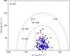 |
Fig. 8. Toomre diagram for the selected stars of the present study (colour-coding as in Fig. 2). Stars are plotted according to their membership probability (> 80%) to belong to the thin disc (solid circles), thick disc (crosses), or halo (triangles) stellar population. Dashed lines indicate |

where σr, σθ, σz are the assumed velocity dispersions of the components (we omitted the i subscript for visibility reasons) and Vi is their mean rotational velocity (i.e. Vθ − Vi estimates the lag compared to the LSR). The assumed values are adopted from Table 6 in Kordopatis et al. (2011). We then compute
 (2)
(2)
If Pi is greater than 80%, we assign to the considered star the membership of the ith component that scored this probability. According to this criterion stars are quoted with a 0, 1, and 2 in Table 1 depending on whether they belong to the thin disc, thick disc, and halo, respectively. We find that N-, SC-, and J-type carbon stars mostly belong to the thin disc, at a rate of 96%, 100%, and 94%, respectively. Two N-type stars (V CrB and RU Vir), both known to be Mira variables, also have typical thick-disc kinematics. Unlike RU Vir, where no metallicity information exists in the literature, V CrB has two measurements: [Fe/H] = −1.3 derived by Abia et al. (2001) and [Fe/H] = −2.12 reported by Kipper (1998). Such a large difference clearly illustrates the problems of the spectroscopic analysis for such cool and chemically complex stars. That said, whether it is −1.3 or −2.12, such a low metallicity for a C-rich Mira is unusual for Galactic stars, and this could suggest that V CrB is an extragalactic interloper (Feast et al. 2006). There are carbon stars in the Galactic halo that are likely to have an extragalactic origin and, at least in the Sagittarius dwarf galaxy, some of them are known to be Miras (Ibata et al. 2001; Whitelock et al. 1999; Mauron et al. 2014). The additional N-type star with probable thick disc membership (see Fig. 8 and Table 1) is V2309 Oph. However, there is no information in the literature about its metallicity. Boffin et al. (1993) found some Li enhancement in this star, log ϵ(Li) ∼ 1.0. The sole J-type star belonging to the thick disc (BM Gem, see Table 1 and Fig. 8) according to our criterion has a metallicity [Fe/H] ∼ +0.2 (Abia & Isern 2000), which we note is typical of thin disc stars.
As far as R-hot stars are concerned, ∼30% of them have a probability higher than 80% to belong to the thick disc, and one of them, HIP 40374, exhibits kinematics fully compatible with the halo (Pi = 100%). In fact, HIP 40374 is frequently considered in the literature as a halo CH-type star (Hartwick & Cowley 1985; Aoki & Tsuji 1997) showing a low 12C/13C∼10, a very common chemical property in CH-type stars. HIP 74826 is slightly metal poor ([Fe/H] = −0.3, Zamora et al. 2009), which is compatible with a thick disc membership. At least six additional R-hot stars (some of them labelled in Fig. 8, see also Table 1) have kinematics compatible with the thick disc. Unfortunately, no information exists in the literature about their chemical composition. Since the Vz velocity component increases with the stellar age (e.g. Nordström et al. 2004), this figure reinforces our previous conclusion (see Sect. 2) that a significant part of the R-hot stars belong to an older (probably less massive) stellar population than the other types of carbon stars.
Figure 9 shows the location above or below the Galactic plane versus the eccentricity of the orbits for the different spectral types. Clearly, it is difficult to distinguish between the N-, SC-, and J-types in this diagram. Most of them have almost circular orbits (e ≲ 0.15) and do not extend beyond |z| ≳ 300 pc from the Galactic plane, this value being the typical scale height of the thin disc (e.g. Jurić et al. 2008). Interestingly enough, SC- stars have eccentricities only within 0.1−0.2. This result, if not related to small number statistics (we recall that we only have ten SC-stars), is difficult to explain otherwise. Considering that the vertical velocity of these stars is relatively low (see also Fig. 10), the fact that we do not find low-eccentricity SC stars could imply that their orbits have been affected by Lindblad resonances with the spiral arms (e.g. Sellwood 2014, and references therein). However, in such a scenario, it would be puzzling why the other carbon stars in our sample have not been affected in a similar fashion. On the other hand, R-hot stars deviate again from the above trend: They have on average a higher eccentricity (⟨e⟩,σ) = (0.17, 0.10) than the other types of carbon stars; (0.10, 0.07), (0.13, 0.10), (0.10, 0.08) for N-, SC- and J-types, respectively. Furthermore, 13 (3.6)14 of these R-hot stars out 35 are located above |z|∼500 pc as opposed to 4 (2) stars out 144 for N-types, and zero out 10 and 21 for both SC- and J-types, respectively. In fact, a similar fit to the |z| distribution above the Galactic plane as already performed for N-type stars (see Sect. 2) gives a scale height zo ≈ 450 pc. Some stars with extreme orbits are also indicated in Figs. 9 and 10. Note that, as expected, these stars are the same as those labelled in Fig. 8 (Table 1) with a possible thick disc membership. Similar conclusions can be drawn from Fig. 10, which illustrates the relationship between the different velocity components: no clear distinction can be noticed between the different carbon star types with velocities typical of the thin disc stars, whereas the R-hot stars show again more heatedVr and Vz distributions.
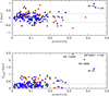 |
Fig. 9. Top: Z-coordinate above and below the Galactic plane vs. eccentricity. Bottom: estimated maximum Z-coordinate along the orbit vs. eccentricity. In the bottom panel the stars V CrB and HIP 40374 are located beyond the Y-axis limits, at |Zmax| = 4.4 and 8.8 kpc, respectively. The horizontal dotted lines in both panels at Z ∼ ±0.3 indicate the commonly accepted scale height of the local thin disc. Colour-coding as in Fig. 2. |
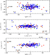 |
Fig. 10. Velocity (radial, orbital, and vertical) diagrams for the sample stars. Orbital velocities refer to the local standard of rest, VθLSR = 240 km s−1. Colour-coding as in Fig. 2. A few objects with peculiar kinematics are labelled. |
5. Characterisation of carbon stars with the Gaia-2MASS diagram
Recently, Lebzelter et al. (2018), using the Gaia DR2 LPV candidates in the Large Magellanic Cloud, showed that an optimal combination of visual and infrared photometry allows the identification of subgroups of AGB stars according to their mass and chemistry (i.e. C- and O-rich AGB stars). These authors adopted a particular combination of Gaia and IR photometry, leading to the infrared Wesenheit function defined as WRP, BP − RP − WKs, J − Ks with
 (3)
(3)
and
 (4)
(4)
where GBP and GRP are the Gaia magnitudes in the blue and the red band, respectively. In the Gaia-2MASS diagram, which plots the Ks-absolute magnitude versus WRP, BP − RP − WKs, J − Ks, the C- and O-rich AGB stars populate different regions, which allows us to easily identify them as long as their distances are known. Furthermore, with the help of synthetic population models (Girardi et al. 2005; Marigo et al. 2017), Lebzelter et al. (2018) show that this diagram also allows the distinction between low-mass, intermediate-mass, and massive O-rich AGB stars as well as super giants and extreme C-rich AGB stars, the specific stellar mass range in each of these groups depending on the stellar metallicity (see Lebzelter et al. 2018, for details). The named extreme C-rich stars concerns very red objects with large (J − Ks) and high mass-loss rates. Recently, Mowlavi et al. (2019) have extended this analysis to the Small Magellanic Cloud and the Galactic LPVs from the full Gaia DR2 archive, showing the power of this diagram in the study of populations harbouring AGB stars. In particular, they found some interesting features in the diagram emerging from the different metallicities in these three stellar systems.
The distribution in the Gaia-2MASS diagram of our sample stars is shown in Fig. 11. For comparison purposes, we have added to the sample a few Galactic O-rich AGB stars (black filled circles, see Sect. 2 and Table 1) presumably of intermediate mass (≳3 − 4 M⊙) according to García-Hernández et al. (2007), fulfilling our parallax quality criterion (see Sect. 2). Dashed lines delimit the regions of different stellar masses identified by Lebzelter et al. (2018) (see their Table 1) for the LPV objects in the LMC, according to the synthetic population models by Marigo et al. (2017). We adopt the same areas here, but we have re-scaled them to the absolute magnitude Ks, assuming that the distance modulus of the LMC is 18.49 (Alves 2004). We note that some differences may exists in these limits when taking into account the difference in metallicity between the main stellar population of the LMC ([Fe/H] ∼ −0.3) and our Galactic stars ([Fe/H] ∼ 0.0), but we do not expect them to be significant. Nevertheless, Mowlavi et al. (2019) find that this difference is indeed observed at the limit separating O-rich and C-rich objects in the Gaia-2MASS diagram (continuous line in Fig. 11) depending on the average metallicity of the stellar population under study. This border is shown to be shifted to slightly larger WRP, BP − RP − WKs, J − Ks values with increasing average metallicity. According to these authors, this limit would be around WRP, BP − RP − WKs, J − Ks ≈ 0.9 mag for Galactic LPVs, as has been set in Fig. 11. Moreover, due to the higher metallicity of the Galactic LPVs, the line delimiting C-rich and extremely C-rich objects (WRP, BP − RP − WKs, J − Ks ≈ 1.7 mag, in Fig. 11) should probably be slightly shifted to lower WRP, BP − RP − WKs, J − Ks values because the mass-loss rate is expected to be favoured for higher metallicities; in Galactic AGB carbon stars, higher mass-loss rates would appear earlier (lower (J − Ks) value) during the AGB phase with respect to those in the MCs.
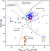 |
Fig. 11. Gaia-2MASS diagram for our sample stars. The curved line delineates the theoretical limit between O-rich (left of the line) and C-rich AGB stars (right of the line). Dashed lines separate subgroups of stars as indicated in the figure. Possible outlier stars are labelled (see text). We have used open blue circles for N-type stars for clarity. Colour code as in Fig. 2 (see text). The uncertainty in MKs is ±0.25 mag typically. |
Figure 11 also shows that the Gaia-2MASS can be used not only to separate O-rich from C-rich objects, but also to identify the different types of carbon stars. N-type stars (blue circles) clearly occupy the whole C-rich region, while the J-type stars (red dots) are located in the same region, but have been shifted a bit to fainter MKs, as discussed in Sect. 3. Remarkably, most of the SC-type stars (green circles), which are characterised by a C/O value very close to unity, are clearly located at the border between O-rich and C-rich objects. The R-hot stars occupy a different region in the RGB and/or faint AGB area compared to the other carbon star spectral types15. Moreover, a considerable number of N-type stars are located in the extreme C-rich zone. According to Lebzelter et al. (2018), these stars would have higher mass-loss rates and, preferably, higher C/O ratios. However, for the stars in our sample with a derived mass-loss rate and a C/O ratio in the literature, we have not found any correlation with the increasing WRP, BP − RP − WKs, J − Ks value. Nevertheless, the N-type stars CW Leo and IY Hya (initially in our sample, but excluded because of their parallax uncertainty), which are known to be extremely red objects with huge mass-loss rates (≳10−5 M⊙ yr−1), are indeed located in this region with WRP, BP − RP − WKs, J − Ks > 4 mag. Clearly, larger and more complete stellar samples are needed to draw a firm conclusion.
The N-type stars TX Psc and V Hya (see Fig. 11) are clearly outside their expected location. Both stars are relatively well-studied carbon stars. The average C/O ratio derived in TX Psc is 1.07 (Klotz et al. 2013), which has been interpreted as evidence of a recent transition from an oxygen-rich to a carbon-rich atmosphere, making TX Psc a relatively “fresh” carbon star. Brunner et al. (2019) have also recently detected an elliptical detached molecular shell around this star and speculate about the possibility of a recent (or a few) TDU episode that transformed it into a C-rich object. Thus, it could be that TX Psc recently became a carbon star and is actually moving rapidly towards the right of the Gaia-2MASS diagram; we have just “caught” it during this move16. V Hya shows evidence of high-velocity, collimated outflows and dense equatorial structures. It is considered as a transition object from an AGB star towards an aspherical planetary nebula (Scibelli et al. 2019). The observed circumstellar structures are also compatible with the existence of a binary companion in an eccentric orbit (Sahai et al. 2016). The impact of the presence of circumstellar structures and binarity on the location of carbon stars in the Gaia-2MASS is beyond the scope of the present study, but the cases of TX Psc and V Hya are quite promising for the use of this diagram, also as a tool to identify “peculiar” AGB stars.
Finally, the few O-rich AGB stars in Fig. 11 are located where they were expected to be. Nevertheless, several studies (García-Hernández et al. 2006, 2007; Pérez-Mesa et al. 2017) point out that some of these stars are intermediate-mass rather than low-mass O-rich AGB stars (i.e. they should be found in Fig. 11 at larger WRP, BP − RP − WKs, J − Ks values and brighter Ks-luminosity). They show strong Li lines and enhanced Rb abundances, which are expected in intermediate-mass (≳3 − 4 M⊙) AGB stars experiencing HBB. Obviously, the small number of O-rich objects in Fig. 11 prevents us from drawing any definitive conclusions.
6. Summary
In this study, we have analysed the Gaia DR2 data for a sample of 210 luminous red giant carbon stars of N, SC, J, and R-hot spectral types belonging to the solar neighbourhood and fulfilling the criterion ϵ(ϖ)/ϖ ≤ 0.2, in order to derive accurate luminosities and kinematic properties. The sample contains variable stars of Mira, irregular, and semi-regular types. Our conclusions can potentially be affected by the accuracy of the distance estimation from Gaia DR2 data and the limited statistics in the case of the SC- and J-type stars. They can be summarised as follows:
We have shown that carbon stars of types N, SC, and J are distributed homogeneously and in a similar way within ∼1.5 kpc of the Sun. A simple exponential fit to the distance from the Galactic plane results in a scale height zo ≈ 180 pc, in agreement with previous determinations. This scale height is compatible with a mass 1.5−1.8 M⊙ for the progenitors of AGB carbon stars at solar metallicity, also in agreement with theoretical expectations. In contrast, we confirm that R-hot stars extend further above or below the Galactic plane, which indicates a lower mass and older population for them.
Carbon stars of N and SC types are well represented by a population having a Gaussian distribution of absolute magnitudes such that (Mbol, σo) = (−5.09, 0.58). Our derived bolometric luminosity function shows two tails at fainter and brighter luminosities that are more extended than previously found. This luminosity function contrasts with the much narrower one derived in Galactic Mira carbon stars (Whitelock et al. 2006), which would constrain this variable type of carbon star to a mass range around ∼2 M⊙. The derived LF implies that Galactic AGB carbon stars may reach up to Mbol ∼ −6.0 mag, a value similar to that found in the Magellanic Clouds. We show that the fainter tail can be understood by considering a contribution of extrinsic low-mass (M ≲ 1 M⊙) carbon stars, while the brighter tail would imply that a non-negligible fraction of stars with initial masses up to 5 M⊙ may become carbon stars during the AGB phase. This would increase the lower mass limit for the occurrence of the HBB to this value, which is in some tension with the extant theoretical models.
Stars of J type are clearly fainter than the N and SC types by about half a magnitude both in Mbol and MK. This is the first time that this figure is clearly shown on an accurate observational basis. This result, together with their very different chemical patterns, confirms that these objects have a different origin, that is still unknown.
We find that R-hot stars have an average ⟨MK⟩ = − 2.54 ± 1.53 mag, which places these stars in the upper part of the RGB. This is about half a magnitude brighter than the value found by Knapp et al. (2001) on the basis of HIPPARCOS parallaxes. This makes it unlikely for these stars to be red-clump objects and the progenitors of J-type stars, as previously suggested.
Our kinematic study shows that the overwhelming majority of the N-, SC-, and J-type stars belong to the thin disc population. To the contrary, a significant fraction (∼30%) of the R-hot stars have kinematics typical of the thick disc, which points towards lower masses and older ages for these objects with respect to the other carbon star types.
Finally, we have shown the potential of the Gaia-2MASS diagram recently used for the LPVs in the Large Magellanic Cloud to identify the different types of carbon stars, which opens an amazing opportunity to identify them in any stellar system as far as accurate distances are known.
There are other types of less evolved carbon stars such as the dwarf carbon stars, CH, Ba, and carbon enhanced metal poor (CEMP) stars. They are main-sequence, subgiants or first-ascend red giant stars and, although they show carbon enhancement, C/O does not necessarily exceed unity in the envelope. We do not study these stars here.
We adopt here the usual notation [X/H] = log (X/H)⋆ – log (X/H)⊙, where (X/H)⋆ is the abundance by number of the element X in the corresponding star.
Very luminous Li-rich carbon stars have also been found in the Magellanic Clouds (Smith et al. 1995).
We do not discuss here the R-cold (or late) carbon stars as it has been shown that they are indistinguishable from the N-type stars (Zamora et al. 2009).
The Two Micron Sky Survey is less sensitive to the detection of R-type stars than to the other carbon star types (Claussen et al. 1987).
We do not expect the proper motions to be affected by this effect as the signature on the sky over the time span of the Gaia DR2 observations allows us to distinguish clearly the proper motion movement from the parallax effect.
We assumed a symmetric uncertainty derived as the average of (rest − rlow) and (rhigh − rest); see Bailer-Jones et al. (2018) for further details.
Luminous (Mbol ≲ −5.8 mag) AGB carbon stars have been found in the Magellanic Clouds (van Loon et al. 1999), some of them exceeding the classical AGB luminosity limit, which could be HBB stars in the latest stage of the AGB phase.
We include here only those carbon stars considered by Gullieuszik et al. (2012) to have dusty envelopes, and therefore more probably placed on the AGB phase.
Although models show that the HBB ceases when the envelope mass is reduced to ∼1 M⊙ (see e.g. Karakas & Lattanzio 2014), the duration of the C-star phase would be too short to provide any sizeable contribution to the LF, but very bright C-stars indeed exist (e.g. IRAS04496–6958 in the LMC with Mbol ∼ −6.8; van Loon et al. 1999; Trams et al. 1999).
At the beginning of the TP-AGB phase of low-mass solar metallicity models, the core mass is around 0.55 M⊙; the models attain the C-rich phase when the core mass is around 0.60 M⊙.
The number within the parenthesis indicates the possible deviation from this figure obtained as  , where N is the number of stars.
We checked that other carbon enriched objects (but not necessarily showing C/O > 1 in their atmosphere) such as CH, Ba, and CEMP stars are also located in this region.
TX Psc is suspected to be a binary star; it is the brightest N-type star in our sample (G = 3.72 mag). Such a bright G-magnitude may be affected by saturation problems that could occur for the brightest Gaia DR2 targets, also affecting the determination of the parallax (Drimmel et al. 2019). These two factors may therefore affect its WRP, BP − RP − WKs, J − Ks value.
Acknowledgments
This work has been partially supported by the Spanish grants AYA2015-63588-P and PGC2018-095317-B-C21 within the European Funds for Regional Development (FEDER) and by the “Programme National de Physique Stellaire” (PNPS) of CNRS/INSU co-funded by CEA and CNES. It has made use of data from the European Space Agency (ESA) mission Gaia (https://www.cosmos.esa.int/gaia), processed by the Gaia Data Processing and Analysis Consortium (DPAC, https://www.cosmos.esa.int/web/gaia/dpac/consortium). Funding for the DPAC has been provided by national institutions, in particular the institutions participating in the Gaia Multilateral Agreement. This research has also made use of the SIMBAD database, operated at CDS, Strasbourg, France. The authors would like to thank the referee, J. T. van Loon, for the careful reading of the manuscript and useful comments and suggestions.
References
- Abia, C., & Isern, J. 2000, ApJ, 536, 438 [NASA ADS] [CrossRef] [Google Scholar]
- Abia, C., & Wallerstein, G. 1998, MNRAS, 293, 89 [NASA ADS] [CrossRef] [Google Scholar]
- Abia, C., Boffin, H. M. J., Isern, J., & Rebolo, R. 1993, A&A, 272, 455 [NASA ADS] [Google Scholar]
- Abia, C., Pavlenko, Y., & de Laverny, P. 1999, A&A, 351, 273 [NASA ADS] [Google Scholar]
- Abia, C., Busso, M., Gallino, R., et al. 2001, ApJ, 559, 1117 [NASA ADS] [CrossRef] [Google Scholar]
- Abia, C., Domínguez, I., Gallino, R., et al. 2002, ApJ, 579, 817 [NASA ADS] [CrossRef] [Google Scholar]
- Abia, C., Domínguez, I., Gallino, R., et al. 2003, PASA, 20, 314 [NASA ADS] [CrossRef] [Google Scholar]
- Abia, C., Cunha, K., Cristallo, S., & de Laverny, P. 2015, A&A, 581, A88 [NASA ADS] [CrossRef] [EDP Sciences] [Google Scholar]
- Abia, C., Straniero, O., & Ventura, P. 2017a, Mem. Soc. Astron. It., 88, 360 [NASA ADS] [Google Scholar]
- Abia, C., Hedrosa, R. P., Domínguez, I., & Straniero, O. 2017b, A&A, 599, A39 [NASA ADS] [CrossRef] [EDP Sciences] [Google Scholar]
- Abia, C., Cristallo, S., Cunha, K., de Laverny, P., & Smith, V. V. 2019, A&A, 625, A40 [NASA ADS] [CrossRef] [EDP Sciences] [Google Scholar]
- Alves, D. R. 2000, ApJ, 539, 732 [NASA ADS] [CrossRef] [MathSciNet] [Google Scholar]
- Alves, D. R. 2004, New Astron. Rev., 48, 659 [NASA ADS] [CrossRef] [Google Scholar]
- Aoki, W., & Tsuji, T. 1997, A&A, 317, 845 [NASA ADS] [Google Scholar]
- Arenou, F., Grenon, M., & Gomez, A. 1992, A&A, 258, 104 [NASA ADS] [Google Scholar]
- Bailer-Jones, C. A. L., Rybizki, J., Fouesneau, M., Mantelet, G., & Andrae, R. 2018, AJ, 156, 58 [NASA ADS] [CrossRef] [Google Scholar]
- Barnbaum, C., Stone, R. P. S., & Keenan, P. C. 1996, ApJS, 105, 419 [NASA ADS] [CrossRef] [EDP Sciences] [Google Scholar]
- Bensby, T., Feltzing, S., & Lundström, I. 2003, A&A, 410, 527 [NASA ADS] [CrossRef] [EDP Sciences] [Google Scholar]
- Bergeat, J., Knapik, A., & Rutily, B. 2001, A&A, 369, 178 [NASA ADS] [CrossRef] [EDP Sciences] [Google Scholar]
- Bergeat, J., Knapik, A., & Rutily, B. 2002, A&A, 390, 967 [NASA ADS] [CrossRef] [EDP Sciences] [Google Scholar]
- Bessell, M. S., & Wood, P. R. 1984, PASP, 96, 247 [NASA ADS] [CrossRef] [Google Scholar]
- Bessell, M. S., Castelli, F., & Plez, B. 1998, A&A, 333, 231 [NASA ADS] [Google Scholar]
- Binney, J. 2012, MNRAS, 426, 1328 [NASA ADS] [CrossRef] [Google Scholar]
- Boffin, H. M. J., Abia, C., Isern, J., & Rebolo, R. 1993, A&AS, 102, 361 [NASA ADS] [Google Scholar]
- Bovy, J. 2015, ApJS, 216, 29 [NASA ADS] [CrossRef] [Google Scholar]
- Boyer, M. L., Girardi, L., Marigo, P., et al. 2013, ApJ, 774, 83 [NASA ADS] [CrossRef] [Google Scholar]
- Brunner, M., Mecina, M., Maercker, M., et al. 2019, A&A, 621, A50 [NASA ADS] [CrossRef] [EDP Sciences] [Google Scholar]
- Busso, M., Gallino, R., Lambert, D. L., Raiteri, C. M., & Smith, V. V. 1992, ApJ, 399, 218 [NASA ADS] [CrossRef] [Google Scholar]
- Buzzoni, A., Patelli, L., Bellazzini, M., Pecci, F. F., & Oliva, E. 2010, MNRAS, 403, 1592 [NASA ADS] [CrossRef] [Google Scholar]
- Capozzi, D., Maraston, C., Daddi, E., et al. 2016, MNRAS, 456, 790 [NASA ADS] [CrossRef] [Google Scholar]
- Castellani, V., Degl’Innocenti, S., Girardi, L., et al. 2000, A&A, 354, 150 [NASA ADS] [Google Scholar]
- Catchpole, R. M., & Feast, M. W. 1971, MNRAS, 154, 197 [NASA ADS] [Google Scholar]
- Cescutti, G., & Molaro, P. 2019, MNRAS, 482, 4372 [NASA ADS] [CrossRef] [Google Scholar]
- Chiavassa, A., Freytag, B., & Schultheis, M. 2018, A&A, 617, L1 [NASA ADS] [CrossRef] [EDP Sciences] [Google Scholar]
- Claussen, M. J., Kleinmann, S. G., Joyce, R. R., & Jura, M. 1987, ApJS, 65, 385 [NASA ADS] [CrossRef] [Google Scholar]
- Cole, A. A., & Weinberg, M. D. 2002, ApJ, 574, L43 [NASA ADS] [CrossRef] [Google Scholar]
- Costa, E., & Frogel, J. A. 1996, AJ, 112, 2607 [NASA ADS] [CrossRef] [Google Scholar]
- Cristallo, S., Piersanti, L., Straniero, O., et al. 2011, ApJS, 197, 17 [NASA ADS] [CrossRef] [Google Scholar]
- Cristallo, S., Straniero, O., Piersanti, L., & Gobrecht, D. 2015, ApJS, 219, 40 [NASA ADS] [CrossRef] [Google Scholar]
- Cutri, R. M., Skrutskie, M. F., van Dyk, S., et al. 2003, VizieR Online Data Catalog: II/246 [Google Scholar]
- Deroo, P., van Winckel, H., Verhoelst, T., et al. 2007, A&A, 467, 1093 [NASA ADS] [CrossRef] [EDP Sciences] [Google Scholar]
- Dominy, J. F. 1984, ApJS, 55, 27 [NASA ADS] [CrossRef] [Google Scholar]
- Dove, J. B., & Thronson, Jr., H. A. 1993, ApJ, 411, 632 [NASA ADS] [CrossRef] [Google Scholar]
- Drimmel, R., Bucciarelli, B., & Inno, L. 2019, Res. Notes Am. Astron. Soc., 3, 79 [Google Scholar]
- Feast, M. W., Whitelock, P. A., & Menzies, J. W. 2006, MNRAS, 369, 791 [NASA ADS] [CrossRef] [Google Scholar]
- Freeman, K., & Bland-Hawthorn, J. 2002, ARA&A, 40, 487 [NASA ADS] [CrossRef] [Google Scholar]
- Frogel, J. A., Persson, S. E., & Cohen, J. G. 1980, ApJ, 239, 495 [NASA ADS] [CrossRef] [Google Scholar]
- Frost, C. A., Cannon, R. C., Lattanzio, J. C., Wood, P. R., & Forestini, M. 1998, A&A, 332, L17 [NASA ADS] [Google Scholar]
- Gaia Collaboration (Helmi, A., et al.) 2018, VizieR Online Data Catalog: 361 [Google Scholar]
- García-Hernández, D. A., García-Lario, P., Plez, B., et al. 2006, Science, 314, 1751 [NASA ADS] [CrossRef] [Google Scholar]
- García-Hernández, D. A., García-Lario, P., Plez, B., et al. 2007, A&A, 462, 711 [NASA ADS] [CrossRef] [EDP Sciences] [Google Scholar]
- Gilmore, G., Wyse, R. F. G., & Kuijken, K. 1989, ARA&A, 27, 555 [NASA ADS] [CrossRef] [Google Scholar]
- Girardi, L., Groenewegen, M. A. T., Hatziminaoglou, E., & da Costa, L. 2005, A&A, 436, 895 [NASA ADS] [CrossRef] [EDP Sciences] [Google Scholar]
- Gontcharov, G. A. 2006, Astron. Lett., 32, 759 [NASA ADS] [CrossRef] [Google Scholar]
- Groenewegen, M. A. T., de Jong, T., van der Bliek, N. S., Slijkhuis, S., & Willems, F. J. 1992, A&A, 253, 150 [NASA ADS] [Google Scholar]
- Groenewegen, M. A. T., Wood, P. R., Sloan, G. C., et al. 2007, MNRAS, 376, 313 [NASA ADS] [CrossRef] [Google Scholar]
- Guandalini, R., & Cristallo, S. 2013, A&A, 555, A120 [NASA ADS] [CrossRef] [EDP Sciences] [Google Scholar]
- Gullieuszik, M., Groenewegen, M. A. T., Cioni, M.-R. L., et al. 2012, A&A, 537, A105 [NASA ADS] [CrossRef] [EDP Sciences] [Google Scholar]
- Hartwick, F. D. A., & Cowley, A. P. 1985, AJ, 90, 2244 [NASA ADS] [CrossRef] [Google Scholar]
- Houdashelt, M. L., Bell, R. A., & Sweigart, A. V. 2000, AJ, 119, 1448 [Google Scholar]
- Ibata, R., Lewis, G. F., Irwin, M., Totten, E., & Quinn, T. 2001, ApJ, 551, 294 [NASA ADS] [CrossRef] [Google Scholar]
- Iben, Jr., I., & Renzini, A. 1983, ARA&A, 21, 271 [NASA ADS] [CrossRef] [Google Scholar]
- Ivezić, Ž., Beers, T. C., & Jurić, M. 2012, ARA&A, 50, 251 [NASA ADS] [CrossRef] [Google Scholar]
- Izzard, R. G., & Tout, C. A. 2004, MNRAS, 350, L1 [NASA ADS] [CrossRef] [Google Scholar]
- Izzard, R. G., Jeffery, C. S., & Lattanzio, J. 2007, A&A, 470, 661 [NASA ADS] [CrossRef] [EDP Sciences] [Google Scholar]
- Izzard, R. G., Jeffery, C. S., & Lattanzio, J. 2008, in Evolution and Nucleosynthesis in AGB Stars, eds. R. Guandalini, S. Palmerini, & M. Busso, Am. Inst. Phys. Conf. Ser., 1001, 33 [NASA ADS] [Google Scholar]
- Javadi, A., & van Loon, J. T. 2020, IAU Symp., 343, in press [arXiv:1811.12025] [Google Scholar]
- Jura, M. 1991, A&ARv, 2, 227 [NASA ADS] [CrossRef] [Google Scholar]
- Jura, M., & Kleinmann, S. G. 1989, ApJ, 341, 359 [NASA ADS] [CrossRef] [Google Scholar]
- Jurić, M., Ivezić, Ž., Brooks, A., et al. 2008, ApJ, 673, 864 [NASA ADS] [CrossRef] [MathSciNet] [Google Scholar]
- Karakas, A. I., & Lattanzio, J. C. 2014, PASA, 31, e030 [NASA ADS] [CrossRef] [Google Scholar]
- Katz, D., Sartoretti, P., Cropper, M., et al. 2019, A&A, 622, A205 [NASA ADS] [CrossRef] [EDP Sciences] [Google Scholar]
- Keenan, P. C. 1993, PASP, 105, 905 [NASA ADS] [CrossRef] [Google Scholar]
- Kerschbaum, F., Lebzelter, T., & Mekul, L. 2010, A&A, 524, A87 [NASA ADS] [CrossRef] [EDP Sciences] [Google Scholar]
- Kipper, T. 1998, Balt. Astron., 7, 435 [NASA ADS] [Google Scholar]
- Klotz, D., Paladini, C., Hron, J., et al. 2013, A&A, 550, A86 [NASA ADS] [CrossRef] [EDP Sciences] [Google Scholar]
- Knapp, G., Pourbaix, D., & Jorissen, A. 2001, A&A, 371, 222 [NASA ADS] [CrossRef] [EDP Sciences] [Google Scholar]
- Kordopatis, G., Recio-Blanco, A., de Laverny, P., et al. 2011, A&A, 535, A107 [NASA ADS] [CrossRef] [EDP Sciences] [Google Scholar]
- Lambert, D. L., Gustafsson, B., Eriksson, K., & Hinkle, K. H. 1986, ApJS, 62, 373 [NASA ADS] [CrossRef] [Google Scholar]
- Lambert, D. L., Smith, V. V., Busso, M., Gallino, R., & Straniero, O. 1995, ApJ, 450, 302 [NASA ADS] [CrossRef] [Google Scholar]
- Lattanzio, J. 2003, in Planetary Nebulae: Their Evolution and Role in the Universe, eds. S. Kwok, M. Dopita, & R. Sutherland, IAU Symp., 209, 73 [NASA ADS] [Google Scholar]
- Lebzelter, T., Mowlavi, N., Marigo, P., et al. 2018, A&A, 616, L13 [NASA ADS] [CrossRef] [EDP Sciences] [Google Scholar]
- Lindegren, L. 2018, Re-normalising the Astrometric Chi-square in Gaia DR2, gAIA-C3-TN-LU-LL-124 [Google Scholar]
- Lindegren, L., Hernández, J., Bombrun, A., et al. 2018, A&A, 616, A2 [NASA ADS] [CrossRef] [EDP Sciences] [Google Scholar]
- Ludwig, H. G. 2006, A&A, 445, 661 [NASA ADS] [CrossRef] [EDP Sciences] [Google Scholar]
- Marigo, P., Girardi, L., & Bressan, A. 1999, A&A, 344, 123 [NASA ADS] [Google Scholar]
- Marigo, P., Girardi, L., Bressan, A., et al. 2017, ApJ, 835, 77 [NASA ADS] [CrossRef] [Google Scholar]
- Mauron, N., Gigoyan, K. S., Berlioz-Arthaud, P., & Klotz, A. 2014, A&A, 562, A24 [NASA ADS] [CrossRef] [EDP Sciences] [Google Scholar]
- McClure, R. D. 1984, in Observational Tests of the Stellar Evolution Theory, eds. A. Maeder, & A. Renzini, IAU Symp., 105, 187 [NASA ADS] [CrossRef] [Google Scholar]
- McSaveney, J. A., Wood, P. R., Scholz, M., Lattanzio, J. C., & Hinkle, K. H. 2007, MNRAS, 378, 1089 [NASA ADS] [CrossRef] [Google Scholar]
- Mengel, J. G., & Gross, P. G. 1976, Ap&SS, 41, 407 [NASA ADS] [CrossRef] [Google Scholar]
- Menzies, J. W., Feast, M. W., & Whitelock, P. A. 2006, MNRAS, 369, 783 [NASA ADS] [CrossRef] [Google Scholar]
- Miller, G. E., & Scalo, J. M. 1979, ApJS, 41, 513 [NASA ADS] [CrossRef] [Google Scholar]
- Montegriffo, P., Ferraro, F. R., Origlia, L., & Fusi Pecci, F. 1998, MNRAS, 297, 872 [NASA ADS] [CrossRef] [Google Scholar]
- Morgan, D. H., Cannon, R. D., Hatzidimitriou, D., & Croke, B. F. W. 2003, MNRAS, 341, 534 [NASA ADS] [CrossRef] [Google Scholar]
- Mowlavi, N., Lecoeur-Taïbi, I., Lebzelter, T., et al. 2018, A&A, 618, A58 [NASA ADS] [CrossRef] [EDP Sciences] [Google Scholar]
- Mowlavi, N., Trabucchi, M., & Lebzelter, T. 2019, 53rd ESLAB Symposium: The Gaia Universe, held 8–12 April, 2019 at ESTEC/ESA, Noordwijk, The Netherlands, 62 [Google Scholar]
- Neugebauer, G., & Leighton, R. B. 1969, Two-micron Sky Survey; A Preliminary Catalog, 3047 [Google Scholar]
- Neyskens, P., Van Eck, S., Plez, B., et al. 2011, J. Phys. Conf. Ser., 328, 012014 [CrossRef] [Google Scholar]
- Nordström, B., Mayor, M., Andersen, J., et al. 2004, A&A, 418, 989 [NASA ADS] [CrossRef] [EDP Sciences] [Google Scholar]
- Ohnaka, K., & Tsuji, T. 1996, A&A, 310, 933 [NASA ADS] [Google Scholar]
- Paczyński, B. 1971, Acta Astron., 21, 1 [NASA ADS] [Google Scholar]
- Pastorelli, G., Marigo, P., Girardi, L., et al. 2019, MNRAS, 485, 5666 [NASA ADS] [CrossRef] [Google Scholar]
- Pérez-Mesa, V., Zamora, O., García-Hernández, D. A., et al. 2017, A&A, 606, A20 [NASA ADS] [CrossRef] [EDP Sciences] [Google Scholar]
- Piersanti, L., Cabezón, R. M., Zamora, O., et al. 2010, A&A, 522, A80 [NASA ADS] [CrossRef] [EDP Sciences] [Google Scholar]
- Platais, I., Pourbaix, D., Jorissen, A., et al. 2003, A&A, 397, 997 [NASA ADS] [CrossRef] [EDP Sciences] [Google Scholar]
- Pourbaix, D., Platais, I., Detournay, S., et al. 2003, A&A, 399, 1167 [Google Scholar]
- Recio-Blanco, A., de Laverny, P., Kordopatis, G., et al. 2014, A&A, 567, A5 [NASA ADS] [CrossRef] [EDP Sciences] [Google Scholar]
- Reid, M. J., & Honma, M. 2014, ARA&A, 52, 339 [NASA ADS] [CrossRef] [Google Scholar]
- Renzini, A. 2015, in Why Galaxies Care about AGB Stars III: A Closer Look in Space and Time, eds. F. Kerschbaum, R. F. Wing, & J. Hron, ASP Conf. Ser., 497, 1 [NASA ADS] [Google Scholar]
- Rowe, J. F., Richer, H. B., Brewer, J. P., & Crabtree, D. R. 2005, AJ, 129, 729 [NASA ADS] [CrossRef] [Google Scholar]
- Sahai, R., Scibelli, S., & Morris, M. R. 2016, ApJ, 827, 92 [NASA ADS] [CrossRef] [Google Scholar]
- Salaris, M., & Girardi, L. 2002, MNRAS, 337, 332 [NASA ADS] [CrossRef] [Google Scholar]
- Samus, N. N., Durlevich, O. V., et al. 2004, VizieR Online Data Catalog: II/250 [Google Scholar]
- Schechter, P. L., Cook, K. H., Aaronson, M., & Blanco, V. M. 1987, BAAS, 19, 1069 [NASA ADS] [Google Scholar]
- Schönrich, R. 2012, MNRAS, 427, 274 [NASA ADS] [CrossRef] [Google Scholar]
- Scibelli, S., Sahai, R., & Morris, M. R. 2019, ApJ, 870, 117 [NASA ADS] [CrossRef] [Google Scholar]
- Sellwood, J. A. 2014, Rev. Mod. Phys., 86, 1 [NASA ADS] [CrossRef] [Google Scholar]
- Sengupta, S., Izzard, R. G., & Lau, H. H. B. 2013, A&A, 559, A66 [NASA ADS] [CrossRef] [EDP Sciences] [Google Scholar]
- Smith, V. V., & Lambert, D. L. 1990, ApJS, 72, 387 [NASA ADS] [CrossRef] [Google Scholar]
- Smith, V. V., Plez, B., Lambert, D. L., & Lubowich, D. A. 1995, ApJ, 441, 735 [NASA ADS] [CrossRef] [Google Scholar]
- Stancliffe, R. J., Izzard, R. G., & Tout, C. A. 2005, MNRAS, 356, L1 [NASA ADS] [CrossRef] [Google Scholar]
- Straniero, O., Domínguez, I., Cristallo, S., & Gallino, R. 2003, PASA, 20, 389 [NASA ADS] [CrossRef] [Google Scholar]
- Straniero, O., Gallino, R., & Cristallo, S. 2006, Nucl. Phys. A, 777, 311 [NASA ADS] [CrossRef] [Google Scholar]
- Trams, N. R., van Loon, J. T., Zijlstra, A. A., et al. 1999, A&A, 344, L17 [NASA ADS] [Google Scholar]
- Van Eck, S., & Jorissen, A. 1999, A&A, 345, 127 [NASA ADS] [Google Scholar]
- Van Eck, S., Jorissen, A., Udry, S., Mayor, M., & Pernier, B. 1998, A&A, 329, 971 [NASA ADS] [Google Scholar]
- van Leeuwen, F. 2007, A&A, 474, 653 [NASA ADS] [CrossRef] [EDP Sciences] [Google Scholar]
- van Loon, J. T., Zijlstra, A. A., Whitelock, P. A., et al. 1997, A&A, 325, 585 [NASA ADS] [Google Scholar]
- van Loon, J. T., Zijlstra, A. A., & Groenewegen, M. A. T. 1999, A&A, 346, 805 [NASA ADS] [Google Scholar]
- Vanture, A. D., Smith, V. V., Lutz, J., et al. 2007, PASP, 119, 147 [NASA ADS] [CrossRef] [Google Scholar]
- Vassiliadis, E., & Wood, P. R. 1993, ApJ, 413, 641 [NASA ADS] [CrossRef] [Google Scholar]
- Ventura, P., Karakas, A. I., Dell’Agli, F., et al. 2015, MNRAS, 450, 3181 [NASA ADS] [CrossRef] [Google Scholar]
- Wallerstein, G., & Knapp, G. R. 1998, ARA&A, 36, 369 [NASA ADS] [CrossRef] [Google Scholar]
- Wallerstein, G., Iben, Jr., I., Parker, P., et al. 1997, Rev. Mod. Phys., 69, 995 [NASA ADS] [CrossRef] [Google Scholar]
- Whitelock, P. A. 2020, IAU Symp., 343, in press [arXiv:1809.10077] [Google Scholar]
- Whitelock, P., Menzies, J., Irwin, M., & Feast, M. 1999, in The Stellar Content of Local Group Galaxies, eds. P. Whitelock, & R. Cannon, IAU Symp., 192, 136 [NASA ADS] [Google Scholar]
- Whitelock, P. A., Feast, M. W., van Loon, J. T., & Zijlstra, A. A. 2003, MNRAS, 342, 86 [NASA ADS] [CrossRef] [MathSciNet] [Google Scholar]
- Whitelock, P. A., Feast, M. W., Marang, F., & Groenewegen, M. A. T. 2006, MNRAS, 369, 751 [NASA ADS] [CrossRef] [EDP Sciences] [Google Scholar]
- Willems, F. J. 1988, A&A, 203, 51 [NASA ADS] [Google Scholar]
- Wojno, J., Kordopatis, G., Steinmetz, M., et al. 2016, MNRAS, 461, 4246 [NASA ADS] [CrossRef] [Google Scholar]
- Wyse, R. F. G., & Gilmore, G. 1995, AJ, 110, 2771 [NASA ADS] [CrossRef] [Google Scholar]
- Zamora, O., Abia, C., Plez, B., Domínguez, I., & Cristallo, S. 2009, A&A, 508, 909 [NASA ADS] [CrossRef] [EDP Sciences] [Google Scholar]
- Zhang, X., & Jeffery, C. S. 2013, MNRAS, 430, 2113 [NASA ADS] [CrossRef] [Google Scholar]
- Zijlstra, A. A., Matsuura, M., Wood, P. R., et al. 2006, MNRAS, 370, 1961 [NASA ADS] [CrossRef] [Google Scholar]
All Figures
|
Fig. 1. Comparison between the HIPPARCOS and the Gaia DR2 parallaxes for 139 stars in common with our sample of Galactic carbon stars. Typical parallax errors are of the order of 50% (or even larger) for HIPPARCOS and smaller than 15% for Gaia. Error bars are omitted in the plot for clarity. The HIPPARCOS parallaxes are systematically larger for sources with Gaia ϖ ≲ 1 mas. See text for details. |
| In the text | |
|
Fig. 2. Left: location of the sample carbon stars of different spectral types on the Galactic plane. The Sun is placed at (X, Y) = (0, 0). Stars shown are N-type (blue); J-type (red); SC-type (green), and R-hot type (brown). Right: distribution above or below the Galactic plane vs. the Galactocentric distance. The Sun is at R = 8.34 kpc. The typical uncertainty in the (X, Y, Z) coordinates is ±20 pc, and ±50 pc for the Galactocentric distance. Two N-type stars with peculiar locations above the Galactic plane are labelled (see text). |
| In the text | |
|
Fig. 3. Luminosity distributions derived in this study for the different spectral types of Galactic carbon stars. The bin size is 0.25 mag. The range of luminosities is different for the R-hot type stars, which are fainter. |
| In the text | |
|
Fig. 4. Derived LF distribution of the present study (blue histogram, excluding J- and R-hot-type stars), compared to those obtained by Gullieuszik et al. (2012) (black dotted line) in the VMC survey of carbon stars, Guandalini & Cristallo (2013) (red dotted line) in Galactic AGB carbon stars, and Whitelock et al. (2006) in Galactic Mira carbon stars (green dashed line). The LFs of these studies have been re-binned with a 0.25 mag step for better comparison. |
| In the text | |
|
Fig. 5. Derived LF for our full sample of Galactic AGB carbon stars (solid black line, excluding J-type and R-hot stars) compared with the theoretical LFs described in Sect. 3 (red dashed histogram), and with the LF expected for a typical model of an extrinsic C-star (black dotted line; see text). The theoretical LFs are normalised such that the peak of a LF matches the peak of the corresponding observations. |
| In the text | |
|
Fig. 6. Bolometric corrections as a function of the effective temperature. Data are from Buzzoni et al. (2010) (red squares) and this study (magenta circles). The new fit (black line) is compared with the one adopted by Straniero et al. (2006) (blue line). See text for details. |
| In the text | |
|
Fig. 7. Evolution of the C/O ratio (upper panels) and surface luminosity (lower panels) for models calculated with different mass-loss laws. See text for details. |
| In the text | |
|
Fig. 8. Toomre diagram for the selected stars of the present study (colour-coding as in Fig. 2). Stars are plotted according to their membership probability (> 80%) to belong to the thin disc (solid circles), thick disc (crosses), or halo (triangles) stellar population. Dashed lines indicate |
| In the text | |
|
Fig. 9. Top: Z-coordinate above and below the Galactic plane vs. eccentricity. Bottom: estimated maximum Z-coordinate along the orbit vs. eccentricity. In the bottom panel the stars V CrB and HIP 40374 are located beyond the Y-axis limits, at |Zmax| = 4.4 and 8.8 kpc, respectively. The horizontal dotted lines in both panels at Z ∼ ±0.3 indicate the commonly accepted scale height of the local thin disc. Colour-coding as in Fig. 2. |
| In the text | |
|
Fig. 10. Velocity (radial, orbital, and vertical) diagrams for the sample stars. Orbital velocities refer to the local standard of rest, VθLSR = 240 km s−1. Colour-coding as in Fig. 2. A few objects with peculiar kinematics are labelled. |
| In the text | |
|
Fig. 11. Gaia-2MASS diagram for our sample stars. The curved line delineates the theoretical limit between O-rich (left of the line) and C-rich AGB stars (right of the line). Dashed lines separate subgroups of stars as indicated in the figure. Possible outlier stars are labelled (see text). We have used open blue circles for N-type stars for clarity. Colour code as in Fig. 2 (see text). The uncertainty in MKs is ±0.25 mag typically. |
| In the text | |
Current usage metrics show cumulative count of Article Views (full-text article views including HTML views, PDF and ePub downloads, according to the available data) and Abstracts Views on Vision4Press platform.
Data correspond to usage on the plateform after 2015. The current usage metrics is available 48-96 hours after online publication and is updated daily on week days.
Initial download of the metrics may take a while.