| Issue |
A&A
Volume 633, January 2020
|
|
|---|---|---|
| Article Number | A57 | |
| Number of page(s) | 9 | |
| Section | Stellar structure and evolution | |
| DOI | https://doi.org/10.1051/0004-6361/201936774 | |
| Published online | 10 January 2020 | |
NICER observations of the Crab pulsar glitch of 2017 November
No. 24, NTI Layout 1st Stage, 3rd Main, 1st Cross, Nagasettyhalli, Bangalore 560094, India
e-mail: This email address is being protected from spambots. You need JavaScript enabled to view it.
Received:
24
September
2019
Accepted:
20
November
2019
Abstract
Context. The Crab pulsar underwent its largest timing glitch on 2017 Nov. 8. The event was discovered at radio wavelengths, and was followed at soft X-ray energies by observatories, such as XPNAV and NICER.
Aims. This work aims to compare the glitch behavior at the two wavelengths mentioned above. Preliminary work in this regard has been done by the X-ray satellite XPNAV. NICER with its far superior sensitivity is expected to reveal much more detailed behavior.
Methods. NICER has accumulated more than 301 kilo seconds of data on the Crab pulsar, equivalent to more than 3.3 billion soft X-ray photons. These data were first processed using the standard NICER analysis pipeline. Then the arrival times of the X-ray photons were referred to the solar system’s barycenter. Then specific analysis was done to study the specific behavior outlined in the following sections, while taking dead time into account.
Results. The variation of the rotation frequency of the Crab pulsar and its time derivative during the glitch is almost exactly similar at the radio and X-ray energies. The following properties of the Crab pulsar remain essentially constant before and after the glitch: the total X-ray flux; the flux, widths, and peaks of the two components of its integrated profile; and the soft X-ray spectrum. There is no evidence for giant pulses at X-ray energies. However, the timing noise of the Crab pulsar shows quasi sinusoidal variation before the glitch, with increasing amplitude, which is absent after the glitch.
Conclusions. Even the strongest glitch in the Crab pulsar appears not to affect all but one of the properties mentioned above, at either frequency. The fact that the timing noise appears to change due to the glitch is an important clue to unravel as this is still an unexplained phenomenon.
Key words: stars: neutron / pulsars: general / pulsars: individual: J0534+2200 / pulsars: individual: B0531+21 / X-rays: stars
© ESO 2020
1. Introduction
On 2017 Nov. 8, a timing glitch occurred in the Crab pulsar that was the largest of the glitches so far (Shaw et al. 2018). They analyzed data for about 150 days after the glitch, and several hundred days before, and brought about the following conclusions that are relevant for this work.
Firstly, the rotation frequency ν rises abruptly at the glitch and decays exponentially, which is similar to other glitches of the Crab pulsar. Most of this rise is abrupt (unresolved in time) while a small part of the rise is delayed and resolved in their data (panel C of Fig. 1, and top panel of Fig. 3, of Shaw et al. 2018). Next, the time derivative of the frequency  reflects the variation of ν on short time scales (< 10 days) – unresolved increase and rapid decrease. On longer timescales, it exponentially recovers to values close to the preglitch value, similar to other glitches of the Crab pulsar (panel D of Fig. 1, and bottom panel of Fig. 3, of Shaw et al. 2018). Further, there is no change in pulse morphology due to the glitch at radio frequencies. The parameters that remain constant across the glitch are the peaks and widths of the main pulse and the inter pulse of the Crab pulsar at 610 and 1520 mega Hertz (MHz) (Fig. 5 of Shaw et al. 2018). Finally, there is no change in the 2 − 50 kilo electron volt (KeV) X-ray flux on account of the glitch (Fig. 6 of Shaw et al. 2018).
Some of these results were confirmed by the X-Ray Pulsar Navigation (XPNAV) satellite (Zhang et al. 2018), whose main purpose was navigation and not astronomy. It nevertheless obtained unprecedented cadence of timing observations at X-ray energies in the range 0.5 − 10 KeV. See their Fig. 3 for the variation in ν and  at the glitch, and their Fig. 5 for constancy of X-ray flux across the glitch.
This work analyses the X-ray data obtained by the Neutron star Interior Composition Explorer (NICER) satellite (Gendreau & Arzoumanian 2017), that is significantly more sensitive than XPNAV, which allows for some analysis that is not possible with XPNAV data. However, NICER is not a dedicated timing instrument, so its cadence of timing observations is nowhere near that of XPNAV.
2. Observations and analysis
NICER consists of 56 coaligned detectors, each of which is essentially a small X-ray telescope (Arzoumanian et al. 2014; Gendreau et al. 2016; Prigozhin et al. 2016). The operating range of NICER is 0.2 − 12 KeV with a peak collecting area of 1900 cm2 at 1.5 KeV, while that of XPNAV is 2.4 cm2 at 1.5 KeV. The time resolution is better than a microsecond (μs); photons are time stamped by an onboard GPS.
At the time of carrying out this work, NICER observed the Crab pulsar on 62 different days, starting from 2017 Aug. 5 to 2019 Apr. 26, which is a duration of 630 days. The first observation was 94 days before the glitch (observation identity number (ObsID) 1013010101, modified Julian date (MJD) 57970.791). There were eight days of observations during 2017 Aug., and two days in 2017 Sep., the last of which occurred on 2017 Sep. 28 (ObsID 1011010201, MJD 58024.575). Then there was a gap of 42 days before the next observation (ObsID 1013010109, MJD 58066.421), which was two days after the glitch (glitch epoch MJD 58064.555), but this observation had a live time of only 224 seconds (s). For the next 11 days, the observations were done daily, after which there was a gap of 40 days (ObsID 1013010122, MJD 58117.329). From then on the observations were mostly on individual days separated by long gaps, except for four continuous days of observation in 2018 Mar., eight continuous days of observation in 2018 Sep., and four continuous days of observation in 2018 Dec. The last observation available for this work was on 2019 Apr. 26 (ObsID 2013010103, MJD 58599.988), but this had only 34 s of live time. This kind of nonuniform cadence of observations implies that one can not perform the phase coherent timing analysis that was done by Shaw et al. (2018) and Zhang et al. (2018). This is particularly true for the glitch that is under discussion; it is so large that the change in phase over a single day can be larger than one cycle so that the cadence required for phase coherent analysis is several timing observations in a single day.
Five of these ObsIDs have live times of 2, 7, 20, 34, and 92 s, and were of no use since one requires at least 100 s of live time on the Crab pulsar to obtain a reasonable integrated profile (IP). In addition, two pairs of observations (ObsIDs 1013010131 and 1013020101 observed on 2018 Apr. 7, and 2013010101 and 2013020101 observed on 2019 Mar. 11) appear to have been observed in some experimental mode – their photon events are not time ordered, but distributed across the two files. So they could not be analyzed together. For Sect. 4, which required the alignment of the data of individual ObsIDs, only those having live times greater than 1000 s were used. This yielded 43 useful ObsIds for analysis. For Sect. 3 which analyses several ObsIDs together, smaller files with at least 100 s of live time could also be used.
The data were analyzed using NICER version five software included in the HEAsoft distribution 6.25; the calibration setup was the CALDB version XTI(20190516). The analysis began with the pipeline tool nicerl2 with default parameters, which selects all 56 detectors, applies standard filters, applies calibration, cleans the events and merges them, etc. Next the average count rate for each detector was calculated using the extractor tool in the light curve mode, and those with counts rates significantly below the mean value are excluded; see Deneva et al. (2019) for details. In the list of 43 ObsIds of Sect. 4, 40 had 52 useful detectors, while two had 51 detectors and one had 50 detectors. Next, light curves were scrutinized for count rates well above and below the mean value. These segments of data were excluded by editing the good times in the tenth HDU (GTI_FILT), and then using the tool fselect with the gtifilter option to filter out photon events outside the good times. The event epochs were then referenced to the solar system barycenter using the barycorr tool using the JPL ephemeris DE431, with the position of the Crab pulsar at that epoch as input.
Finally, an approximate period (1/ν) is estimated (at a nominal period derivative ( )) for each ObsID by first obtaining the power spectrum of the data using the powspec tool. This is refined by searching for maximum probability of period using the efsearch tool. This is further refined by cross correlating the first and second halves of the data (see Vivekanand 2015 for details). These intermediate period and period derivative (or alternately the intermediate ν and
  ) are the starting point for the analysis of the following sections.
2.1. Dead time
An important advantage of NICER’s design is that the effective dead time is very low (LaMarr et al. 2016; Stevens et al. 2018). However this has not been estimated quantitatively so far for the Crab pulsar. Figure 1 shows the dead time for the longest observation in the data set.
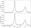 |
Fig. 1. Dead time estimation for the data of ObsID 1013010147. Top panel: IP of the Crab pulsar using the appropriate values of ν and |

Typically, each photon event of NICER results in a dead time of about 15 or 22 μs for each detector (LaMarr et al. 2016); practically the dead time is larger. Now the typical photon count rate per detector, for the Crab nebula plus the Crab pulsar, can be estimated by dividing the total number of photons obtained in Fig. 1 by the live time and by the number of detectors, which is 260699397/23722.5/52 ≈ 211.3 counts per second per detector. This implies a mean interval of about 4.7 milliseconds (ms) between photons. Clearly the dead time is a negligible fraction of this interval, so the dead time correction to the observed count rate would also be negligible. Because the dead time is such a small value, it scales almost linearly with the photon count rate in each phase bin of the IP in Fig. 1, as expected. The offpulse dead time, in the phase range 0 − 0.2, is 0.46 per cent (%) of the live time; at the peak of the Crab pulsar’s pulse the dead time fraction is 0.73%.
These numbers are consistent with the expected values. A Poisson process with mean interval between events τ has an exponential probability density distribution for the time interval between any two events: 1/τ × exp(−t/τ). So the fraction of events that fall during the dead time, say T s, is (by simple integration) ≈T/τ. Now, the mean dead time for the above ObsID is T = 23.1 ± 4.2 μs, and τ = 4.7 ms, so the mean dead time fraction is  %. This work estimates the dead time as a function of the phase of the Crab pulsar’s pulse for each ObsID, and uses it for correction throughout this work, although it is indeed a negligible value.
3. Stride fit
The top and bottom panels of Fig. 3 of Shaw et al. (2018) display the long term variation of ν and  , respectively, at radio wavelengths. The top and bottom panels of Fig. 3 of Zhang et al. (2018) do the same at soft X-ray energies. Shaw et al. (2018) obtain their results by what they label as the “striding boxcar” fit, which essentially fits their timing residuals in smaller but overlapping segments of epochs. Thus they fit timing residuals for 20 consecutive days to a second order polynomial to obtain the ν and
  at the central epoch of the data. They repeat the exercise after sliding the 20 day “boxcar” by five days, to obtain the ν and
  at the next epoch; this implies a 15 day overlap of data between adjacent boxcars. This is done after averaging their original data to just two timing residuals per day, for higher sensitivity to explore the long term variation. Zhang et al. (2018) do the same stride fit, but their boxcar is four days long, with sliding step of half a day.
Figure 2 shows the results of applying the stride fit technique to NICER data of the Crab pulsar. Since the data cadence is highly nonuniform and inadequate, only that data is analyzed in this section that consists of at least two days of consecutive observations. The boxcar width used is three days, except when only two days are possible; the sliding step is one day. Timing residuals are estimated for each 100 s of data within the boxcar, provided the actual live time within the 100 s is at least 90 s. Further details of the stride fit analysis are given in Appendix A.
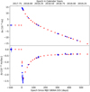 |
Fig. 2. Variation of ν and |


The dots in Fig. 2 are the departures of ν and  values tabulated in the so called Jodrell Bank Crab Pulsar Monthly Ephemeris1 (Lyne et al. 1993; henceforth JBCPME), with respect to the preglitch timing model. This is obtained by fitting the frequency and its first two time derivatives, at the glitch epoch, to data 700 days prior to the glitch; these values (ν0,
  and
and  ) are given in Table 1. The departures Δν and
  vary as in Fig. 3 of Shaw et al. (2018).
The preglitch reference timing model, obtained using ν from JBCPME (Lyne et al. 1993) for ≈700 days before the glitch.
The values of ν0,  and
and  of Shaw et al. (2018) are given in their Table 1. Propagating them from their reference epoch to the glitch epoch, their ν0 differs from the value in Table 1 above by −0.492 micro Hertz (μHz); their
  differs from the above value by 0.042 × 10⁻¹² Hz s−1. These two values are negligible compared to the scale of Δν and
  in Fig. 2, respectively. Strictly, however, they are significant compared to their formal errors. The
  of Shaw et al. (2018) is an order of magnitude larger than the value in Table 1.
Undertaking a similar exercise for the preglitch parameters of Zhang et al. (2018), their ν0 differs from the value in Table 1 above by −0.490 μHz; their  differs from the above value by −0.005 × 10⁻¹² Hz s−1. The
  of Zhang et al. (2018) is an factor of two smaller than the value in Table 1.
I believe these differences arise from the fact that firstly, the ν values listed by the JBCPME (from which Table 1 is derived) are themselves average values, mostly monthly averages, and secondly the preglitch durations of the three works may differ significantly; this may particularly affect the frequency second derivative. It is therefore concluded that there is broad agreement between the preglitch parameters derived here with those of Shaw et al. (2018) and Zhang et al. (2018), at least for the purpose of this work.
The boxes in Fig. 2 are the departures Δν and  estimated from NICER data, with respect to the preglitch timing model given in Table 1. The agreement between the dots (radio data) and the boxes (soft X-ray NICER data) is excellent, not just very close to the glitch but also almost 500 days away from it. The XPNAV data covered only 100 days after the glitch; within these 100 days, Fig. 2 above is both qualitatively and quantitatively consistent with Fig. 3 of Zhang et al. (2018). This section therefore concludes that the variation of ν and
  of the Crab pulsar during the glitch of 2017 Nov. 8 is very similar at the radio and X-ray energies, right from ≈100 days before the glitch to almost 500 days afterward.
4. Pulse properties
At 610 MHz radio frequency, the IP of the Crab pulsar consists of a main pulse; an inter pulse about 0.4 phase cycles after the main pulse, of about half the amplitude; and a much smaller third component known as the precursor leading the main pulse by 0.04 phase cycles (Shaw et al. 2018). All three components are very narrow compared to one phase cycle. At 1520 MHz the precursor almost disappears. Shaw et al. (2018) investigate the possibility of these components changing due to the glitch. They model the two main components using gaussians, and plot their widths, and ratio of their peaks, at both radio frequencies, as a function of epoch at a cadence of once a day (see their Fig. 5). They find no evidence of any change in these parameters on account of the glitch.
Shaw et al. (2018) also plot the daily X-ray flux of the Crab pulsar, in the energy range 15 − 50 KeV, from the Burst Alert Telescope (BAT) instrument aboard the Swift X-ray satellite, as well as the daily X-ray flux in the energy range 2 − 20 KeV from the Monitor of All-sky X-ray Image (MAXI) instrument aboard the International Space Station (ISS); see their Fig. 6. They conclude that there is no change in the X-ray flux of the Crab pulsar that can be associated with the glitch. Zhang et al. (2018) plot five day averages of the onpulse flux in the energy range 0.5 − 10 KeV, and notice no significant change in X-ray flux of the Crab pulsar due to the glitch; see their Fig. 5.
Figure 3 shows the IP of the Crab pulsar for the data of ObsID 1013010143, after folding at the ν and  derived in the previous section, and after aligning it with the IP in Fig. 1 using cross-correlation, and after subtracting the offpulse flux as described later. There are only two pulse components at soft X-rays, and both are fairly wide and appear merged into each other. For the purpose of this section, the two pulse components are defined as follows. First, the minimum of the X-ray flux between the two peaks is identified, by fitting a second order polynomial to the flux data in the phase range 0.475 − 0.625. This is the solid red curve between the two pulse components in Fig. 3. Differentiating this curve gives the phase of minimum flux, which is identified by the middle vertical dashed line in Fig. 3; the horizontal dashed line represents the minimum flux at this phase.
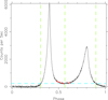 |
Fig. 3. Integrated profile of the Crab pulsar for the data of ObsID 1013010143. The solid red curve between the two pulse components, and the horizontal and vertical dashed lines define the two pulse components for the purpose of parameter estimation; they are explained in the text. |
Next the two outer intersection points of the horizontal dashed line with the IP are estimated, after passing the IP data through a moving average filter of three phase bins, to reduce noise; these are the first and third vertical dashed lines in Fig. 3. Then the main and inter pulses of the Crab pulsar’s IP are identified as lying between the first two and last two vertical dashed lines, respectively. The onpulse flux of the Crab pulsar is defined as lying beyond the phase 0.2.
This procedure is applied to data of each ObsID that has live time > 1000 s, after aligning (using cross-correlation) its IP with the reference IP in Fig. 1, viz. that of ObsID 1013010147, and after subtracting the average offpulse flux in phase range 0.0 − 0.2. Then the following seven parameters are estimated: the average fluxes of the main pulse, the inter pulse and the onpulse; and the rms widths and peaks of the main and inter pulse.
Figure 4 shows the results of this section. The top panel displays the average onpulse X-ray flux of the Crab pulsar per detector. The variation of the data is consistent with it being essentially constant. The total range of data is 13.03 − 12.61 = 0.42 photons per second per detector, while the rms of these data values is 0.09; so the data is spread over 0.42/0.09 = 4.7 standard deviations. Now, for 43 data points one expects a spread over at least three standard deviations. The rest is probably due to factors such as time variability of the calibration of the 56 individual detectors, day and night differences in calibration of NICER, etc. Although there are only six of the 43 points before the glitch, the variation of the data is similar before and after the glitch. It is therefore clear that there is no significant variation of this parameter due to the glitch. This is consistent with the results of Shaw et al. (2018) and Zhang et al. (2018).
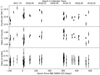 |
Fig. 4. Variation of pulse properties as a function of epoch. Top to bottom panels: average onpulse X-ray flux of the Crab pulsar (photons per second per detector in the energy range 0.2 − 12 KeV), ratio of the average fluxes of the main and inter pulse, and ratio of the rms widths of the main and inter pulse, respectively. |
The middle panel of Fig. 4 shows the ratio of the average fluxes of the main and inter pulse. This is close to the value one because the inter pulse is wider although its peak is smaller. The bottom panel of Fig. 4 shows the ratio of the rms widths of the main and inter pulse. These two parameters also do not display any significant variation due to the glitch. This is also consistent with the results of Shaw et al. (2018). Since the lower two panels of Fig. 4 imply that (consequently) the ratio of the peaks of the two components would also be constant, this result has not been plotted in Fig. 4.
5. Soft X-ray spectrum
This section investigates whether the soft X-ray spectrum of the Crab pulsar changes during the glitch. The calibrated spectrum has to be obtained using the tool xspec. However, it is known that these are early days for the NICER project, and their spectrum calibration is still preliminary. See Sect. 2.1 and Fig. 1 of Ludlam et al. (2018), and Sect. 3 of Miller et al. (2018); see also the pdf file available in nicer_arfrmf_20180329.tar.gz at the NICER archive site2, and NICERDAS-CalibGuide-20180814.pdf at the NICER calibration site3. Even though it is possible that several calibrations issues may have been resolved in the later calibration files that are used in this work, the analysis of this section is performed on both the calibrated as well as the raw spectrum of the Crab pulsar.
One begins the analysis by repeating the initial procedure of Sect. 4 – data of each ObsID is folded at the appropriate ν and  , and shifted in phase using cross-correlation so that its IP is aligned to the reference profile in Fig. 1. Then the phase of each photon is written into an additional column in the event file. This file is filtered in phase using the tool fselect to produce two event files – one with phase ≤0.2 and another with phase > 0.2, corresponding to offpulse and onpulse, respectively. These event files are input to the tool extractor used in the spectrum mode, to produce the corresponding offpulse and onpulse raw spectra. To use them in xspec, the live times of these files have to be corrected – the “EXPOSURE” keyword in the off and on spectra is multiplied by the factor 0.2 and 0.8, respectively, and inserted using the tool fparkey.
Next, the keywords “RESPFILE” and “ANCRFILE” in the onpulse spectrum are set to the current “RMF”4 and “ARF”5 spectrum calibration files, respectively. Finally the “BACKFILE” keyword in the onpulse spectrum is set to the offpulse spectrum. This ensures that when the onpulse spectrum file is defined as the data in xspec, it automatically picks up the offpulse spectrum as the background spectrum, and also picks up the appropriate spectrum calibration files.
Finally, each onpulse spectrum is analyzed using xspec, which is run in the “PYTHON” environment, using the “from xspec import *” command in PYTHON, which picks up the PYTHON libraries from the HEAsoft 6.25 environment if the latter has been installed properly. Channels below 30 and above 600 are ignored, the abscissa is set to the energy mode (“Plot.xAxis = Kev”), and channel dependent effective area is set (“Plot.area = True”). Then the energy, count rate and its error are printed out. The top panel of Fig. 5 displays the calibrated spectrum for ObsID 1013010147.
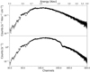 |
Fig. 5. Calibrated (top panel) and uncalibrated (bottom panel) spectrum of ObsID 1013010147. |
The uncalibrated spectrum (bottom panel of Fig. 5) is obtained by removing the response file (“Spectrum.response = None”) and resetting the abscissa to channel mode (“Plot.xAxis = channel”). The uncalibrated spectrum can also be obtained by extracting the raw counts in each channel from the onpulse and offpulse spectra, using the ftlist tool, then dividing them by the respective live times, and then subtracting the two values; this is essentially what xspec also does, apart from calibration. As a consistency check, the integrated photon count rate of the uncalibrated spectrum (over all channels) should agree with the values in the top panel of Fig. 4, after accounting for (a) number of detectors, and (b) the fact that onpulse photons in Fig. 5 arrive during only 80% of the period, while in Fig. 4 they are assumed (correctly) to arrive over the entire period, in order to estimate the average count rate.
Figure 6 shows the result of comparing the calibrated spectrum of each ObsID with that of the reference ObsID (1013010147). The top panel of Fig. 6 shows the χ2 per degree of freedom after subtracting the calibrated spectrum of each ObsID from the calibrated spectrum of the reference ObsID (1013010147). The values are very close to 1.0, with negligible error on them since the number of degrees of freedom is 570. The mean preglitch and postglitch χ2 values are 0.99 and 1.03, with standard deviations 0.06 and 0.07 respectively. The bottom panel conducts the same comparison in a different way. The calibrated spectrum of each ObsID is divided by the calibrated spectrum of the reference ObsID (1013010147), channel by channel, and the average ratio across the spectrum is plotted. The values lie close to 1.0; the mean preglitch and postglitch ratios are 1.01 and 1.00, with standard deviations 0.01 and 0.01 respectively. In both panels of Fig. 6, the scale of variation is similar before and after the glitch.
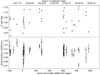 |
Fig. 6. Variation of spectral properties as a function of epoch. Top panel: normalized χ2 after subtracting the reference calibrated spectrum from the calibrated spectrum of the rest of the ObsIDs. Bottom panel: average Ratio after dividing the calibrated spectrum of each ObsID with the reference calibrated spectrum. |
Figure 6 has also been produced using the uncalibrated spectra, and the results are almost identical. This section therefore concludes that there is no difference in the soft X-ray spectrum of the Crab pulsar before and after the glitch.
6. Giant pulses
The Crab pulsar emits at radio frequencies what are known as giant pulses; their amplitude is orders of magnitude larger than that of the mean radio pulse. These occur only within the main pulse and inter pulse, which at radio frequencies are very narrow windows in phase. The radio peaks are aligned with the corresponding peaks at X-rays (Lundgren et al. 1995; Sallmen et al. 1999; Hankins 2000; Cordes et al. 2004; Karuppusamy et al. 2010). Several attempts to detect giant pulses in X-rays and γ-rays have proved futile (Bilous et al. 2012; Mickaliger et al. 2012; Ahronian et al. 2018).
Figure 7 top panel shows the IP of the Crab pulsar (in arbitrary units) using most of the data acquired by NICER, after aligning the IP of each ObsID with that of the reference ObsID 1013010147, using cross-correlation. Visual inspection of the IP, particularly in the phase range 0.2 centered at the main and inter pulses (see Fig. 2 of Mickaliger et al. 2012; see also Sect. 7 of Cordes et al. 2004), revealed no indication of an excess emission. One expects this excess emission to be confined to a few phase bins that represent the domain of arrival of giant pulses.
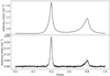 |
Fig. 7. Test for giant pulses. Top panel: integrated profile of the Crab pulsar in soft X-rays, using 289.3 Ks of data (3181769922 photons from 51 ObsIDs) in 1024 phase bins. Bottom panel: difference between the IP of the top panel, and the IP obtained by including only those photons that differ in arrival times by less than 1 μs from each other, after proper scaling, as explained in the text. |
To investigate this issue more quantitatively, an IP was formed from the data using only those photons that differed in arrival times by less than one μs from each other. If the giant pulse phenomenon at radio wavelengths implies more simultaneous photons at X-rays also, then the second IP should show an excess at the phases where giant pulses are expected. This IP contained a factor of ≈24 less photons than that in the top panel of Fig. 7. After proper scaling of both IPs (total area under the IPs should be 1.0) and subtracting, and after introducing a scaling constant, the result obtained is shown in the bottom panel of Fig. 7. There is no excess of photons that is confined to very few channels; the excess is spread over the phase ranges of the main and inter pulses, which is expected naturally because the probability of arrival of closely spaced photons increases with increasing photon count. The photons in the bottom panel of Fig. 7 arrive on different detectors, since on any single detector the time interval between any two photons can not be less than the dead time (15 or 22 μs).
7. Timing noise
Timing noise is the slow and irregular variation of the rotation frequency (ν) of a pulsar (Lyne et al. 1993; Hobbs et al. 2010; Shannon & Cordes 2010; Melatos & Link 2014), unlike the abrupt change in ν at a glitch, and is as yet an unexplained phenomenon. Here it is demonstrated that the largest glitch in the Crab pulsar may have modified its timing noise.
Figure 8 shows the timing noise of the Crab pulsar for 1200 days. The preglitch data is identical to the preglitch data in the top panel of Fig. 2, where only 100 days of this data are displayed. The postglitch data in Fig. 8 are the residuals obtained after fitting Eq. (1) of Vivekanand (2015) (or Eq. (1) of Zhang et al. 2018) to the postglitch data in the top panel of Fig. 2, using the glitch parameters given in Table 2. The fit is done to data from 20 to 554 days after the glitch epoch. Data from the glitch epoch to day 20 varies quite differently, as is evident in the top panel of Fig. 2, but is more clearly apparent in panel C of Fig. 1 of Shaw et al. (2018). Attempt was made to fit this data in two segments – data from glitch epoch to day five, and data from day five to day 20. The resulting residuals were very noisy, and so have been omitted from Fig. 8.
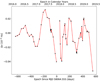 |
Fig. 8. Timing noise of the Crab pulsar for about 3.5 years centered on the glitch. |
The above fit excludes the latest reasonably sized glitch on MJD 58687.59 but includes the two much smaller glitches on MJDs 58237.357 and 58470.939, which fall on days 172.8 and 406.4 in Fig. 8. Their magnitudes are 0.008 and 0.005 fraction of the largest glitch.
The slow and stochastic changes in the ν of the Crab pulsar with respect to its secular variation are evident, with time scales of ≈ a few hundred days before the glitch, and shorter time scales after the glitch, even if one restricted oneself to the range 20–172 days after the glitch. The quasi sinusoidal variation before the glitch, with increasing amplitude, is absent after the glitch. However, since the data of two small glitches have been included in this analysis, the postglitch results of this section can only be tentative.
The difference in preglitch and postglitch Δν in Fig. 8 can not be attributed to any difference in analysis method. Firstly, there is no bias in actual stride lengths between preglitch and postglitch analysis. Secondly, the X-ray data in Fig. 8 (points having larger error bars) fall very close to their corresponding radio points (having no visible error bars at all), when the two observational epochs nearly coincide, say at epochs −100 and 500 days along abscissa.
8. Discussion
The summary of this work is the following. Firstly, the ν and  of the Crab pulsar vary similarly at the radio and soft X-ray energies, during the glitch of 2017 Nov. 8. Secondly, the following properties of the Crab pulsar remain essentially constant before and after the glitch: (a) the total onpulse X-ray flux, (b) the flux of the two components of its integrated profile, (c) the widths and peaks of these two components, and (d) the soft X-ray spectrum. Thirdly, there is no evidence for giant pulses at X-ray energies. Finally, the timing noise appears to change after the glitch. The following discussion focuses on three aspects of the radio and X-ray emission of the Crab pulsar, and on the requirement for X-ray timing observations of rotation powered pulsars.
8.1. Overall emission
Even the strongest glitch in the Crab pulsar (comparable to those occurring in the Vela pulsar) does not change several emission parameters discussed above, both at radio as well as X-ray energies. This is consistent with the belief that both emissions occur very close to each other in the pulsar’s magnetosphere. This has been independently demonstrated by Rots et al. (2004) and Bilous et al. (2012), who show that the separation in phase between the X-ray and radio peaks is 0.01, the radio peak arriving later, so the two emission regions are separated by ≈0.01/29.63 * 3 × 105 ≈ 100 kilometers (km), which is a small fraction of the light cylinder radius in the Crab pulsar (≈1600 km).
The results of this work are also consistent with the belief that both emissions occur far away from the surface of the neutron star, say in the outer gaps (Romani & Watters 2010), since any effect of the glitch is more likely to occur closer to the surface of the neutron star. However, this argument needs to be considered with some caution. Only two pulsars (out of about two thousand) have shown glitch associated radiative changes, and as argued by Shaw et al. (2018), it is not clear why a fractional increase of ≈10−6 in rotation frequency at the surface of the neutron star should induce changes in the pulsar magnetosphere that could affect the pulsar emission.
Since the X-ray spectrum is also unchanged on account of the glitch, the electric fields that accelerate electrons and positrons in the outer gaps, their energy distribution, and the magnetic field in the magnetosphere where they emit X-rays, all three remain the same before and after the glitch. However, the charged particles begin their life at the surface of the neutron star, in the polar cap (Romani & Watters 2010), so if the glitch is accompanied by a re-arrangement of the surface (say a star quake), some of the above three parameters are likely to get affected. Even then, we are unlikely to observe the consequences if the intense gravity at the surface of the neutron star re-adjusts the surface on time scales of, say, 1000 s, which is the time required to obtain a significant integrated profile.
8.2. Giant pulses
The phenomenon of radio giant pulses does not yet have an explanation; see Lundgren et al. (1995), Bilous et al. (2012), and Mickaliger et al. (2012) and references therein for some possibilities. The absence of simultaneous giant pulses at X-rays and γ-rays could imply that coherent bunching of emitting particles might occur on length scales that are much smaller than radio wavelengths, but much larger than X-ray wavelengths. Before proceeding further it should be mentioned that some evidence for giant pulses has been reported at optical wavelengths (Shearer et al. 2003). Here it is argued that there may be instrumental selection effects in observing giant pulses at X-rays.
Let us consider the various possibilities at X-rays that can accompany a radio giant pulse, if the two are indeed correlated. First, there can be multiple X-ray photons emitted simultaneously; Fig. 7 tries to explore this possibility. However, the veto sections of X-ray detectors may discard such photons, because they might be misconstrued for high energy particles, depending upon how many photons there are and what their energy is and what kind of detectors are used, unless there is reasonable time separation between the simultaneous photons. Moreover, this time separation must be larger than the dead time of the detector. The design of NICER drastically reduces the dead time problem – there are several detectors to receive the simultaneous photons. However, if the giant pulses at X-rays are emitted by a coherent mechanism (such as in a laser), and they all happen to fall on one single detector of NICER, then one might have to once again face the veto and dead time aspects of the X-ray detector.
Next, instead of several simultaneous X-ray photons, maybe only a single higher energy photon is emitted; this speculation is not unjustified since we do not know the exact mechanism of giant pulse emission. Then, once again depending upon the actual situation, the photon may either get vetoed, or it falls in a higher energy channel. In this case, one would be looking for excess photons in a region of the spectrum that naturally has very few photons, due to the spectral index of the Crab pulsar at X-ray energies. An inspection of the spectrum for the combined data in Fig. 7 revealed no such excess. If the energy of such a photon is larger than 12 KeV, then NICER would anyway not detect it.
Finally, a radio giant pulse may be accompanied by just a single average energy X-ray photon. In this best scenario situation, the better way of looking for giant pulses using NICER may be to observe simultaneously at radio and X-rays and look for photons that are correlated at both wavelengths, as was done by Lundgren et al. (1995), Bilous et al. (2012), Ahronian et al. (2018).
8.3. Pre glitch timing noise
The preglitch timing noise in Fig. 8 looks like an oscillating signal with increasing amplitude. This requires two ingredients for explanation – an oscillator, and a positive feed back system.
Ruderman (1970) proposed that the quasi periodic timing in the Crab pulsar could be due to Tkachenko oscillations, in which the vortices remain parallel to the rotation axis, but their density (and therefore the angular momentum of the fluid) are redistributed periodically. Equation (7) of Ruderman (1970) shows that the periods of these oscillations are ≈120 days, which is similar in order of magnitude to the ≈200 days quasi periodicity seen before the glitch.
Other modes of oscillation, such as the Kelvin modes or the r-modes, have periods much much smaller than the above values (Ruderman 1970; Haskell & Melatos 2015; Haskell & Sedrakian 2018). Therefore, for the purpose of this discussion Tkachenko oscillations are assumed to be operative before the glitch; however, see Haskell (2011) for the effect of vortex pinning and fluid compressibility, and maybe even entrainment, on the viability of these oscillations.
Next one needs a positive feed back system, something that pumps energy into the oscillator at the correct phase to enhance the amplitude. It is speculated here that this could probably be due to some vortices that are pinned strongly, and therefore are not moving, but are still executing the Tkachenko oscillations, albeit weakly, due to the “knock on” effect of vortices that are in the process of creating an “avalanche”; see Haskell & Melatos (2015), Haskell & Sedrakian (2018) for details. These vortices might strain the crustal lattice, and could create small cracks in it, which would create heat that is pumped into the super fluid system. This periodic thermal pulse could create a periodic bias in the potential in which the vortices are “creeping” (Alpar et al. 1984). Depending upon the actual numbers and one’s imagination, one could believe in the possibility of a positive feed back.
Two points need to be clarified regarding the above speculation. First, the vortices providing the positive feed back are not the ones that are annihilating themselves while depositing angular momentum into the crust. They belong to a different domain in the neutron star, they are pinned to the crust, and they merely sense the Tkachenko oscillations, by virtue of being connected to the super fluid. The high thermal conductivity of the neutron star might ensure that this heat percolates into the neighboring domains where the vortices are free to move. Second, the scale of this activity is orders of magnitude smaller than the scale of the glitch of 2017 Nov. 8 – see the difference in the scale of the ordinates in Figs. 2 and 8. Finally, it is interesting that, while the giant glitch of 2017 Nov. 8 in the Crab pulsar does not fall within the epoch predicted by Vivekanand (2017), one smaller and one relatively larger glitch (MJDs 58470.939 and 58687.59)6 lie within the uncertainty of prediction.
8.4. Importance of X-ray timing observations
Most rotation powered pulsars are easier to observe at radio frequencies than at X-ray energies, for reasons of sensitivity, cost and convenience. However there are several scientific reasons for observing them at X-rays also. Firstly, in some pulsars like the Crab, glitches are believed to be triggered by cracking of the crust of the neutron star, which can lead to bursts of X-ray emission (Ruderman 1991). Therefore X-ray study of pulsar glitches is important to understand their trigger mechanism. Next, the much wider main and inter pulse of the Crab pulsar at X-rays, relative to their radio counterparts, implies that study of pulse morphology variation at X-rays might sense the properties of a much larger volume of the pulsar magnetosphere, than such studies at radio frequencies. Finally, optical and X-ray studies of giant pulses in pulsars might reveal the size of the basic unit of emission, if the phenomenon is due to decreasing coherence of the emission region at increasing frequencies of observation.
nixtiref20170601v001.rmf.
nixtiaveonaxis20170601v002.arf.
Acknowledgments
I thank Marco Antonelli and Brynmor Haskell for useful discussion regarding the role of vortices in the neutron star super fluid. I thank the referee for useful discussion.
References
- Alpar, M. A., Pines, D., Anderson, P. W., & Shaham, J. 1984, ApJ, 276, 325 [NASA ADS] [CrossRef] [Google Scholar]
- Ahronian, F., Akamatsu, H., Akimoto, F., et al. 2018, PASJ, 70, 15 [NASA ADS] [Google Scholar]
- Arzoumanian, Z., Gendreau, K. C., Baker, C. L., et al. 2014, Proc. SPIE, 9144, 914420 [Google Scholar]
- Bilous, A. V., McLaughlin, M. A., Kondratiev, V. I., et al. 2012, ApJ, 749, 24 [NASA ADS] [CrossRef] [Google Scholar]
- Cordes, J. M., Bhat, N. D. R., Hankins, T. H., et al. 2004, ApJ, 612, 375 [NASA ADS] [CrossRef] [Google Scholar]
- Deneva, J. S., Ray, P. S., Lommen, A., et al. 2019, ApJ, 874, 160 [NASA ADS] [CrossRef] [Google Scholar]
- Gendreau, K., Arzoumanian, Z., Adkins, P. W., et al. 2016, Proc. SPIE, 9905, 99051H [Google Scholar]
- Gendreau, K., & Arzoumanian, Z. 2017, Nat. Astron., 1, 895 [NASA ADS] [CrossRef] [Google Scholar]
- Hankins, T. H. 2000, in Pulsar Astronomy - 2000 and Beyond, eds. M. Kramer, N. Wex, & N. Wielebinski, ASP Conf. Ser., 202, 165 [NASA ADS] [Google Scholar]
- Haskell, B. 2011, Phys. Rev. D, 83, 043006 [NASA ADS] [CrossRef] [Google Scholar]
- Haskell, B., & Melatos, A. 2015, Int. J. Mod. Phys. D, 24, 1530008 [NASA ADS] [CrossRef] [Google Scholar]
- Haskell, B., & Sedrakian, A. 2018, in Superfluidity and Superconductivity in Neutron Stars, Astrophys. Space Sci. Lib., 401, 457 [Google Scholar]
- Hobbs, G., Lyne, A. G., & Kramer, M. 2010, MNRAS, 402, 1027 [NASA ADS] [CrossRef] [Google Scholar]
- Karuppusamy, R., Stappers, B. W., & van Straten, W. 2010, A&A, 515, A36 [NASA ADS] [CrossRef] [EDP Sciences] [Google Scholar]
- LaMarr, B., Prigozhin, G., Remillard, R., et al. 2016, Proc. SPIE, 9905, 99054W [Google Scholar]
- Ludlam, R. M., Miller, J. M., Arzoumanian, Z., et al. 2018, ApJ, 858, L5 [NASA ADS] [CrossRef] [Google Scholar]
- Lundgren, S. C., Cordes, J. M., Ulmer, M., et al. 1995, ApJ, 453, 433 [NASA ADS] [CrossRef] [Google Scholar]
- Lyne, A. G., Pritchard, R. S., & Graham Smith, F. 1993, MNRAS, 265, 1003 [NASA ADS] [CrossRef] [Google Scholar]
- Melatos, A., & Link, B. 2014, MNRAS, 437, 21 [NASA ADS] [CrossRef] [Google Scholar]
- Mickaliger, M. B., McLaughlin, M. A., Lorimer, D. R., et al. 2012, ApJ, 760, 64 [NASA ADS] [CrossRef] [Google Scholar]
- Miller, J. M., Gendreau, K., Ludlam, R. M., et al. 2018, ApJ, 860, L28 [NASA ADS] [CrossRef] [Google Scholar]
- Prigozhin, G., Gendreau, K., Doty, J. P., et al. 2016, Proc. SPIE, 9905, 99051I [Google Scholar]
- Romani, R. W., & Watters, K. P. 2010, ApJ, 714, 810 [NASA ADS] [CrossRef] [Google Scholar]
- Rots, A. H., Jahoda, K., & Lyne, A. G. 2004, ApJ, 605, L129 [NASA ADS] [CrossRef] [Google Scholar]
- Ruderman, M. 1970, Nature, 225, 619 [NASA ADS] [CrossRef] [Google Scholar]
- Ruderman, M. 1991, ApJ, 382, 587 [NASA ADS] [CrossRef] [Google Scholar]
- Sallmen, S., Backer, D. C., Hankins, T. H., et al. 1999, ApJ, 517, 460 [NASA ADS] [CrossRef] [Google Scholar]
- Shannon, R. M., & Cordes, J. M. 2010, ApJ, 725, 1607 [NASA ADS] [CrossRef] [Google Scholar]
- Shaw, B., Lyne, A. G., Stappers, B. W., et al. 2018, MNRAS, 478, 3832 [NASA ADS] [CrossRef] [Google Scholar]
- Shearer, A., Stappers, B., O’Connor, P., et al. 2003, Science, 301, 493 [NASA ADS] [CrossRef] [Google Scholar]
- Stevens, A. L., Uttley, P., Altamirano, D., et al. 2018, ApJ, 865, L15 [NASA ADS] [CrossRef] [Google Scholar]
- Vivekanand, M. 2015, ApJ, 806, 190 [NASA ADS] [CrossRef] [Google Scholar]
- Vivekanand, M. 2017, A&A, 597, L9 [NASA ADS] [CrossRef] [EDP Sciences] [Google Scholar]
- Zhang, X., Shuai, P., Huang, L., et al. 2018, ApJ, 866, 82 [NASA ADS] [CrossRef] [Google Scholar]
Appendix A: Details of stride fitting
The stride fitting procedure is applied to the data of usually three, but sometimes two, consecutive ObsIDs. First, one has to estimate the initial ν and  valid for all three (or two) ObsIds, starting from the intermediate ν and
  of each ObsID that are derived in Sect. 2. It was found that for most of the data the initial
  (Table 1) was a good starting point. This value had to be modified only for data close in epoch to the epoch of minimum
  in the lower panel of Fig. 2. Using this value of initial
  , that value of initial ν was obtained, which best aligned the data of all three (or two) ObsIDs. The cross correlation of the IPs of the first and second halves of the combined data was used as a measure of the alignment. These initial ν and
  are referenced to the epoch at the middle of the combined data. Figure A.1 is a contour plot of the combined data of the ObsIDs 1013010116, 1013010117, and 1013010118. The initial ν = 29.6364286361 Hz and the initial
  Hz s−1; the latter is different from the
  of Table 1 to enhance the phase variation, for better viewing.
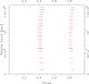 |
Fig. A.1. Contour plot of the combined data of the ObsIDs 1013010116, 1013010117, and 1013010118, after alignment using initial ν and |

Next, IPs are formed from data of 100 s duration, using the initial ν and  , and the phase of the main pulse is obtained by fitting a Gaussian to the peak (see Vivekanand 2015 for details); this phase is plotted in Fig. A.2 as a function of epoch, relative to the mid epoch of the combined data. The phase data shows the characteristic quadratic behavior expected for deviations of ν and
  from their initial values. A second order polynomial is fit to this phase data, to obtain the final ν and
  . It is essentially to such data that Shaw et al. (2018) and Zhang et al. (2018) have fit a second order polynomial, to obtain their ν and
  as a function of epoch.
In Fig. A.2, a correction to ν will shift the position of minimum phase away from the origin. It is clear that this correction is quite small; it turn out to be −0.019(2) μHz. The correction to  is 0.104(1)×10−10 Hz s−1. It is important to get the initial values of ν and
  as close as possible to the final values. Otherwise, the quadratic curve would be shifted away from the origin and there is a chance of the higher phase values becoming larger than 1.0, in which case they are folded over to very small values in the next cycle.
All Tables
The preglitch reference timing model, obtained using ν from JBCPME (Lyne et al. 1993) for ≈700 days before the glitch.
All Figures
|
Fig. 1. Dead time estimation for the data of ObsID 1013010147. Top panel: IP of the Crab pulsar using the appropriate values of ν and |
| In the text | |
|
Fig. 2. Variation of ν and |
| In the text | |
|
Fig. 3. Integrated profile of the Crab pulsar for the data of ObsID 1013010143. The solid red curve between the two pulse components, and the horizontal and vertical dashed lines define the two pulse components for the purpose of parameter estimation; they are explained in the text. |
| In the text | |
|
Fig. 4. Variation of pulse properties as a function of epoch. Top to bottom panels: average onpulse X-ray flux of the Crab pulsar (photons per second per detector in the energy range 0.2 − 12 KeV), ratio of the average fluxes of the main and inter pulse, and ratio of the rms widths of the main and inter pulse, respectively. |
| In the text | |
|
Fig. 5. Calibrated (top panel) and uncalibrated (bottom panel) spectrum of ObsID 1013010147. |
| In the text | |
|
Fig. 6. Variation of spectral properties as a function of epoch. Top panel: normalized χ2 after subtracting the reference calibrated spectrum from the calibrated spectrum of the rest of the ObsIDs. Bottom panel: average Ratio after dividing the calibrated spectrum of each ObsID with the reference calibrated spectrum. |
| In the text | |
|
Fig. 7. Test for giant pulses. Top panel: integrated profile of the Crab pulsar in soft X-rays, using 289.3 Ks of data (3181769922 photons from 51 ObsIDs) in 1024 phase bins. Bottom panel: difference between the IP of the top panel, and the IP obtained by including only those photons that differ in arrival times by less than 1 μs from each other, after proper scaling, as explained in the text. |
| In the text | |
|
Fig. 8. Timing noise of the Crab pulsar for about 3.5 years centered on the glitch. |
| In the text | |
|
Fig. A.1. Contour plot of the combined data of the ObsIDs 1013010116, 1013010117, and 1013010118, after alignment using initial ν and |
| In the text | |
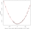 |
Fig. A.2. Phase of the main pulse of the IP of 100 s duration, of the data in Fig. A.1. |
| In the text | |
Current usage metrics show cumulative count of Article Views (full-text article views including HTML views, PDF and ePub downloads, according to the available data) and Abstracts Views on Vision4Press platform.
Data correspond to usage on the plateform after 2015. The current usage metrics is available 48-96 hours after online publication and is updated daily on week days.
Initial download of the metrics may take a while.