| Issue |
A&A
Volume 633, January 2020
|
|
|---|---|---|
| Article Number | A146 | |
| Number of page(s) | 11 | |
| Section | Galactic structure, stellar clusters and populations | |
| DOI | https://doi.org/10.1051/0004-6361/201936294 | |
| Published online | 24 January 2020 | |
The nature of the NGC 2546: Not one but two open clusters⋆⋆⋆
1
Facultad de Ciencias Exactas, Físicas y Naturales, Universidad Nacional de San Juan, Complejo Universitario “Islas Malvinas”, Av. Ignacio de la Roza Oeste 590, J5402DCS San Juan, Argentina
e-mail: This email address is being protected from spambots. You need JavaScript enabled to view it.
2
Instituto de Ciencias Astronómicas, de la Tierra y del Espacio (ICATE-Universidad Nacional de San Juan), Av. España Sur 1512, J5402DSP San Juan, Argentina
Received:
10
July
2019
Accepted:
10
December
2019
Abstract
Context. As part of a broader project on the role of binary stars in clusters, we present a spectroscopic study of the open cluster NGC 2546, which is a large cluster lacking previous spectroscopic analysis.
Aims. We report the finding of two open clusters in the region of NGC 2546. For the two star groups, we determine radial velocity, parallax, proper motion, reddening, distance modulus, and age, using our spectroscopic observations and available photometric and astrometric data, mainly from the second Gaia data release (Gaia-DR2). We also determine the orbit of four spectroscopic binaries in these open clusters.
Methods. From mid-resolution spectroscopic observations for 28 stars in the NGC 2546 region, we determined radial velocities and evaluate velocity variability. To analyze double-lined spectroscopic binaries, we used a spectral separation technique and fit the spectroscopic orbits using a least-squares code. The presence of two stellar groups is suggested by the radial velocity distribution and confirmed by available photometric and astrometric data. We applied a multi-criteria analysis to determine cluster membership, and obtained kinematic and physical parameters of the clusters.
Results. NGC 2546 is actually two clusters, NGC 2546A and NGC 2546B, which are not physically related to each other. NGC 2546A has an age of about 180 Myr and a distance of 950 pc. It has a half-number radius of 8 pc and contains about 480 members brighter than G = 18 mag. NGC 2546B is a very young cluster (<10 Myr) located at a distance of 1450 pc. It is a small cluster with 80 members and a half-number radius of 1.6 pc. Stars less massive than 2.5 M⊙ in this cluster would be pre-main-sequence objects. We detected four spectroscopic binaries and determined their orbits. The two binaries of NGC 2546A contain chemically peculiar components: HD 68693 is composed of two mercury-manganese stars and HD 68624 has a Bp silicon secondary. Among the most massive objects of NGC 2546B, there are two binary stars: HD 68572, with P = 124.2 d, and CD -37 4344 with P = 10.4 d.
Key words: binaries: spectroscopic / stars: chemically peculiar / open clusters and associations: individual: NGC 2546 / techniques: radial velocities / surveys
Tables 2 and 3 are only available at the CDS via anonymous ftp to cdsarc.u-strasbg.fr (130.79.128.5) or via http://cdsarc.u-strasbg.fr/viz-bin/cat/J/A+A/633/A146
This work is based on observations obtained at the Complejo Astronómico El Leoncito, operated under an agreement between the Consejo Nacional de Investigaciones Científicas y Técnicas de la República Argentina and the National Universities of La Plata, Córdoba and San Juan.
© ESO 2020
1. Introduction
The present work is part of a wider project aimed at detecting and characterizing spectroscopic binaries in open clusters. Besides the impact that interactive binaries have on stellar evolution giving rise to a variety of exotic stellar products, the binary population, in general, is of particular importance in the dynamical evolution of the clusters (Leigh & Geller 2012, 2013). The empirical knowledge on this matter, however, is scarce (Duchêne & Kraus 2013) since extensive spectroscopic observations and a proper membership analysis are required. Such detailed studies are lacking even for many bright clusters.
This is the case of NGC 2546, a large cluster with relatively bright stars (the main-sequence extends to V ∼ 8 mag) that has been largely neglected. Among the 236 clusters listed by Piskunov et al. (2007), for example, only ∼10% have a larger mass and tidal radius than NGC 2546. Less than 4% of the clusters included in the WEBDA database have a larger angular diameter. In fact, the high angular diameter of open clusters often hamper their study since extended clusters have a stronger field star contamination and are more difficult to study photometrically with standard detectors.
NGC 2546 was studied by Lindoff (1968) through UBV photographic photometry. He measured 1047 stars, finding 85 probable members spread on an elongated area of 25′ × 50′. This author determined a true distance modulus of 9.95 mag (d = 980 pc), a reddening of E(B − V) = 0.17 mag and an age of log(τ) = 7.3. In this paper, we use the identification numbers of that work.
Beyond that early work and the photoelectric search for Ap stars by Maitzen (1982), no other specific study of this cluster has been carried out. Several of the brightest stars, however, have UBV photoelectric magnitudes obtained in different surveys (e.g., Lodén 1969). On the other hand, there is no previous spectroscopic study devoted to this cluster. The Michigan Catalogue of spectral types (Houk 1982) includes fifteen stars in the field of the cluster, among which there are three silicon stars (stars 30, 322, and 544). Accurate radial velocities have only been obtained for the two giant stars 99 and 356 by Mermilliod et al. (2008), while a handful of bright stars have been measured on photographic plates by Harris (1976).
In the present paper, we expose the results of our spectroscopic study of this cluster, including the detection of new spectroscopic binaries and the identification of two different stellar groups. In Sect. 2 and 3, we describe the spectroscopic observations and the orbital analysis of binary stars. In Sect. 4, we combine our spectroscopic data with other available information to discuss cluster membership on a basis of multiple criteria. The main conclusions are summarized in Sect. 5.
2. Spectroscopy
The spectroscopic analysis of NGC 2546 is based on 177 spectra collected between the years 2000 and 2018. These observations were carried out using the 2.15 m telescope and the REOSC echelle spectrograph at the CASLEO, San Juan, Argentina. The spectra cover the wavelength range 3700–6300 Å with a resolving power R = 12 400. The data were reduced by using standard tasks of the NOAO/IRAF package. The final steps of the data processing included combination of the echelle orders, spectrum normalization, cosmic rays remotion, and heliocentric velocity correction.
We determined spectral types for the 28 observed stars using the criteria of Gray & Corbally (2009), Jaschek & Jaschek (2009), and Sota et al. (2014). In the case of broad-line stars, we compared the object spectrum with spectra of standard stars observed with the same instrument and convolved with appropriate rotational profiles. The spectral types obtained are listed in Table 1. Cases of uncertain classification (mostly due to low signal-to-noise ratio or high rotational velocity) are marked with a colon.
Results obtained from spectroscopy and membership analysis.
We measured radial velocities (hereafter RVs) by cross-correlation using the IRAF task fxcor. The selection of spectral regions for the correlations depended on the line width. For spectra with line profiles of FWHM (full-width at half-maximum) < 200 km s−1 we excluded hydrogen lines, interstellar lines, and regions lacking lines. On the other hand, for spectra with FWHM > 200 km s−1 we used mainly helium and hydrogen lines. The relative velocity between object and template was measured by fitting a Gaussian to the correlation peak. The template spectra for the cross-correlations were selected from database of Bertone et al. (2008). In high rotation stars, synthetic templates were previously convolved with appropriate rotational profiles. All RV measurements are listed in Table 2 (single stars) and Table 3 (double lined spectroscopic binaries), available at the CDS. The errors listed were calculated as the quadratic sum of the measurement error given by the task fxcor and an error of 0.7 km s−1 related to the centering of the star on the slit. This value was estimated by González & Lapasset (2000) for the instrument used under standard conditions.
For each star we calculated the average velocity ( ) and its uncertainty (
 ) using the expressions of González & Lapasset (2000). In those equations the error is calculated taking into account both the individual errors and the dispersion of the measurements. We adopted the criterion of that paper to classify a star as an RV variable. The results of these calculations are listed in Table 1. Stars 9, 134, and 277 are classified as RV variable (var). These stars could be single-lined spectroscopic binaries (SB1s), so further observational monitoring is desirable to confirm their binarity and, in such a case, determine their orbits. However, from our membership analysis we concluded that the star 9 is not a cluster member. We note that several stars classified as RV constant have only two measurements. The variability classification must be considered as preliminar for these stars.
3. Spectroscopic binaries
The sample of 28 stars observed contains three double-lined spectroscopic binaries (SB2s) and one single-lined binary (SB1). For SB2s we used the spectral separation technique described by González & Levato (2006). This method allows to measure RVs even in spectra where the separation between the components in the spectrum is comparable to the width of the lines.
The detection of the binary nature of stars 30 and 257 was not trivial, since the spectral features of the two companions strongly overlap, and the spectral lines of the primary “hide” those of its companion. In these systems, the binarity was suspected from line profile variations detected on the basis of 2–5 observations per star taken in the first observing runs, and consequently, they were monitored in subsequent runs. As illustration, we show in Fig. 1 the spectra obtained in that first spectroscopic survey of the cluster along with the final spectra of the components, reconstructed combining all observations with the method mentioned above. The systems are close to the resolution limit, with RV differences smaller than the width of the lines. Besides the careful inspection of the line profiles, the identification of small spectral lines that are not present in the primary (because of the difference in spectral type) helped to detect the binary nature of the star 30. Afterward, the binarity was definitely confirmed by the convergence of the iterative disentangling and by the morphology of the reconstructed spectra of the companions. We note that if in these stars RV measurements are made by standard correlations with templates of the same line-width, they would be classified as RV constant.
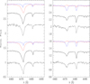 |
Fig. 1. Spectral separation of the SB2s 30 (right panel) and 257 (left panel). Two observed spectra taken at different orbital phases are plotted for each star. The reconstructed spectra of the two stellar component are shown in blue and red. Below, in thin black line, is the spectrum modeled combining the two spectra of the components, and below it, in heavy black line, the observed spectrum. |
Once the RVs of both components were obtained, we used the IRAF task pdm to identify the orbital period of the system. Then we fit the spectroscopic orbits using our own least-squares FORTRAN code. The orbital elements obtained for the three SB2 stars (stars 10, 30, and 257) and the SB1 star 475 are listed in Table 4. The RV curves are showed in Fig. 2. Only one of the four spectroscopic binaries detected, star 10, had been previously reported in González & González (2012). The components of this binary are both chemically peculiar of the HgMn type.
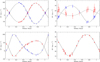 |
Fig. 2. Radial velocity curves of the four studied binaries: NGC 2546−10 (upper left), NGC 2546−30 (upper right), NGC 2546−257 (lower left), and NGC 2546−475 (lower right). |
Orbital parameters for SB.
4. Membership
4.1. Radial velocities
To calculate the cluster mean RV and determine kinematic membership, we analyzed the RV distribution of the observed stars. For each star we considered the mean RV in the case of constant stars and the center-of-mass velocity for the four spectroscopic binaries. For the two RV variables we adopted different criteria. In the case of the star 134, we fit several possible orbits to the measured RVs, obtaining that the center-of-mass velocities were, in all cases, very close to the mean RV computed. Therefore, we included that value in the calculation. On the other hand, we discarded the more uncertain mean RV of the star 277. The RV distribution is shown in Fig. 3, where each star is represented by a Gaussian whose width σ is related to the uncertainty of its mean RV. The global distribution (sum of all Gaussians) is clearly bimodal, suggesting the presence of two stellar groups with RVs of about 16 and 26 km s−1, which we call NGC 2546A and NGC 2546B, respectively. Blue and red lines in the figure represent the distribution of bona fide members, what exclude stars rejected by other membership criteria (see further below).
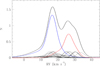 |
Fig. 3. RV distribution of observed objects. Each star is represented by a Gaussian whose width depends on the RV error. Heavy black line is the global RV distribution. Blue and red lines show the distributions of stars classified as members of the clusters NGC 2546A and NGC 2546B, respectively. |
The cluster NGC 2546A is well represented kinematically by five stars with mean RV determined better than 1.1 km s−1: three late-B type stars (stars 10, 30, and 134) and two red giants (stars 99 and 356). Their average RV is 16.3 km s−1 with σ = 1.0 km s−1. The stellar group NGC 2546B can be defined by the three early-B type stars 257, 259, and 475, whose mean RV is 26.3 km s−1 with σ = 0.9 km s−1. The late-B type star 544 has a RV consistent with this group, but is not a cluster member as shown below. The massive star 682, a photometric member of this group, has a RV somewhat higher (30.5 ± 0.8 km s−1). Taking into account these parameters, we selected as probable RV members those stars whose RV difference with the cluster mean is smaller that its uncertainty. In the final calculation of the RV of the cluster we included all stars classified as members (see Table 1). Since RV uncertainties vary considerably from star to star, in the cluster mean we applied weights proportional to (ε2 + Δ2)−1, where ε is the uncertainty of the star RV and Δ = 1 km s−1. The reason of including the constant Δ is that the RV of an individual star, as an estimator of the mean cluster velocity, has a uncertainty of at least the internal velocity of the cluster, which is typically on the order of 1 km s−1 in open clusters. The final values for the mean RV of the clusters are 16.5 ± 0.5 km s−1 and 26.3 ± 0.6 km s−1.
Only three stars of NGC 2546A have RVs in the second Gaia data release (Gaia-DR2) with uncertainties below 8 km s−1, the two red giants and one main-sequence star not observed by us. The RVs of the red giants 99 and 356 (16.67 ± 0.12 km s−1 and 15.18 ± 0.18, respectively) are in excellent agreement with our results (16.83 ± 0.46 km s−1 and 15.20 ± 0.36 km s−1). The third star is TYC 7660-2144-1, whose RV in Gaia is 20.8 ± 1.9 km s−1.
4.2. Reddening
As a second criterion to evaluate the existence of two stellar groups and asign membership, we analyzed the interstellar reddening of early-type stars. We did not use the photographic photometry by Lindoff (1968) because of its low quality. Instead, we used photoelectric UBV measurements from different sources (Claria 1985; Lodén 1969; Schild et al. 1983; Fernie 1979, priv. comm.; Oja 1976, priv. comm.). Figure 4 shows the color–color diagram for stars with available photoelectric UBV photometry.
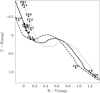 |
Fig. 4. Color–color diagram obtained with the available photoelectric photometry and the standard sequence of Schmidt-Kaler (1982). The dashed line corresponds to E(B − V) = 0.00, the black and gray continuous lines correspond to E(B − V) = 0.14 mag and E(B − V) = 0.29 mag respectively. |
The standard sequence of Schmidt-Kaler (1982) shifted according to E(B − V) = 0.00, 0.14, and 0.29 is shown for comparison. This diagram shows two stellar sequences with different interstellar extinction suggesting, alike the RV distribution, the presence of two clusters. The four OB type stars 266, 272, 475, and 682 define a sequence different than that of stars of later spectral types. Using the Q method (Johnson & Morgan 1953) we determined individual values of E(B − V) for all early-type stars with available UBV magnitudes (see Table 5). The mean values obtained are E(B − V) = 0.140 ± 0.006 mag for NGC 2546A and E(B − V) = 0.292 ± 0.004 mag for NGC 2546B.
Interstellar extinction obtained with the Q method.
4.3. Spectroscopic distance modulus
We used the Schmidt-Kaler calibration to estimate absolute magnitudes MV and intrinsic colors (B − V)0 from spectral types. Combining these values with apparent magnitudes and colors we derived the reddening and distance modulus. The results are shown in Fig. 5.
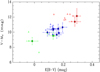 |
Fig. 5. Spectroscopic reddening and distance modulus. Filled circles are stars with photoelectric photometry. Blue, red, and green symbols are stars belonging to NGC 2546A, NGC 2546B, and the galactic field, respectively, according to our multicriteria final assignment. Open triangles correspond to Tycho magnitudes (see text). |
Unfortunately, less than half of our spectroscopic targets have reliable photometric data. Filled circles in the figure are stars with photoelectric photometry. The cluster NGC 2546A is well represented; the mean reddening and distance modulus for this cluster are E(B − V) = 0.15 and (V − MV) = 10.20, while the true distance modulus is 9.74 ± 0.21 mag. In these calculation we excluded red giant stars, whose spectroscopic absolute magnitudes have large uncertainties, and star 313, which is a field star according to parallax and proper motion (See Sect. 4.4).
Only two probable members of NGC 2546B have photoelectric photometry: stars 475 and 682. For that reason, we consider that this method does not give meaningful information for this cluster. Nonetheless, it might be mentioned that the distance modulus obtained for these two stars is consistent with the value derived from other methods.
In order to verify the presence of two groups in our spectroscopic sample, we calculated reddening and distance modulus using Tycho magnitudes BT and VT, which were transformed to Johnson B and V following Bessell (2000). These data are plotted with open triangles in Fig. 5 and show clearly the two clusters.
4.4. Proper motion and parallax
The definitive identification of the stellar clusters NGC 2546A and B was made using Gaia DR2 data (Gaia Collaboration 2018a). The stars mentioned above, which distinguished kinematically the two clusters, also defined two distinct groups in the proper motion space, as can be seen in Fig. 6. The five RV members of NGC 2546A are marked with filled blue circles. Open blue circles represent stars whose mean RVs have errors larger than 1.1 km s−1 but are consistent with the cluster velocity (stars 90, 112, 322, 354, and 448). Red diamonds are probable (kinematic or photometric) members of the young cluster NGC 2546B (stars 257, 259, 266, 272, 277, and 475). As in the previous case, open diamonds distinguish stars with greater errors in mean RV. The massive star 682 (filled red square) is probable member according to photometric and proper motion criteria, while its RV is about 4 km s−1 higher than other probable members. Proper motions and/or spectroscopic distance modulus discard as member of either of the two clusters the three A-type stars 201, 380, and 575, the Bp star 544, and the giant star 540.
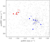 |
Fig. 6. Proper motion of RV members of the two clusters. Blue circles are RV members of NGC 2546A; filled circles are stars with RV uncertainties below 1.1 km s−1. Red diamonds are RV members of NGC 2546B; the filled red square is the O-type star 682. The other stars are Gaia sources with magnitude G < 14 mag. |
In order to define the mean proper motion and parallax of the two clusters we analyzed Gaia data in a circle of 1° radius centered at the nominal coordinates of the cluster (α2000 = 08h12m15s,  ). In a first approach we used only stars brighter than G = 14 mag in order to reduce the field star contamination. Figure 7 shows the Gaia proper motion distribution, where both star clusters are detectable. To calculate the barycenter of the clusters we built a continuous proper motion distribution by replacing each point by a Gaussian of σ = 0.1 mas yr−1. Then we fit the observed distribution with two Gaussians representing the cluster under consideration and the local field distribution. The proper motion distribution along the vertical and horizontal sections shown in blue and red in Fig. 7 are plotted in Fig. 8. As an statistical confirmation of the existence of two clusters, we applied to the parallax distribution a two-sample Kolmogorov–Smirnov test to the two star groups defined by proper motions, obtaining that the probability that the two samples belong to the same parent population is less than 1.0 × 10⁻⁴.
 |
Fig. 7. Proper motion distribution of Gaia stars brighter than G = 14 mag. The position of clusters NGC 2546A and NGC 2546B are at the intersection of continuous red lines and dashed blue lines, respectively. |
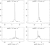 |
Fig. 8. Sections of the proper motion distribution along the vertical and horizontal lines shown in Fig. 7. Upper panels correspond to NGC 2546A and lower panels to NGC 2546B. |
The parallax distribution of all stars brighter than G = 14 mag is shown in the upper panel of Fig. 9. The histogram has been plotted using an adaptive smoothing kernel (K-nearest-neighbors).
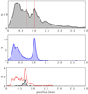 |
Fig. 9. Parallax distribution of stars within a circle of 1 deg radius. Upper panel: stars brighter than G = 14 mag. Vertical lines mark the position of the two clusters. Middle panel: stars brighter than G = 16 mag with proper motion consistent with the cluster NGC 2546A. Lower panel: stars brighter than G = 16 mag with proper motion consistent with NGC 2546B in a circle of 1 deg radius (red curve) and in a 0.1 deg radius circle centred in the coordinates of NGC 2546B (gray filled curve). |
In order to obtain star samples that are clean and large enough to determine the mean cluster parallax, we extended the limiting magnitude to G = 16 mag but restricted the sample to probable proper-motion members of each cluster. We considered stars in a circle of 0.5 mas yr−1 radius around the cluster mean in the proper-motion space. The stars of NGC 2546A selected in this way are distributed covering a wide area in the sky but they are numerous enough to define a clear peak in the parallax distribution, as can be seen in the second panel of Fig. 9. In the case of the cluster NGC 2546B the number of stars is smaller but their spatial distribution much more concentrated. We show in Fig. 10 the position in the sky of stars with proper motions compatible with the cluster NGC 2546B. From this point distribution we derived preliminar coordinates of the cluster center and selected those lying within a 0.1 deg radius circle to analyze the parallax distribution. The resulting sample shows a clear concentration in parallax with a mean value of 0.70 mas (lower panel of Fig. 9). The mean cluster parallax was calculated for each cluster by fitting a Gaussian (plus a linear background) to these distributions, obtaining 1.03 for NGC 2546A and 0.69 mas for NGC 2546B.
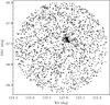 |
Fig. 10. Spatial distribution of stars with G < 16 mag and proper motion compatible with the cluster NGC 2546B. |
Using the Tycho-Gaia Astrometric Solution, Cantat-Gaudin et al. (2018) determined for NGC 2546 a mean parallax of 0.98 ± 0.07 mas, which is in line with the value computed in this work for NGC 2546A. This is not the case for the proper motion, since the mean values of μα and μδ obtained by those authors are intermediate between those computed by us for the two clusters.
4.5. Astrometric errors
The diameter of both clusters is small enough compared to the distance, so that the observed star-to-star dispersion in parallax (about 0.06 mas), is a measure of the typical internal uncertainty of Gaia data. However, the uncertainty of the cluster mean parallax cannot be calculated as usual by dividing the rms by the square root of the number of stars, since Gaia data suffer of various systematic errors, both global and depending on the sky position, as have been reported in several works (see for example Lindegren et al. 2018; Gaia Collaboration 2018b; Arenou et al. 2018; Luri et al. 2018).
According to Lindegren et al. (2018), there exist systematic errors that depend on the celestial coordinates mainly on two different scales. On the one hand, there are modulations on scales of tens of degrees with amplitudes of 0.017 mas in parallax and 0.028 mas yr−1 in proper motions and, on the other hand, a periodic pattern with a period close to 1 deg and amplitudes of 0.043 mas and 0.066 mas yr−1. These smaller scale errors have less impact on the cluster mean parameters in the case of large clusters. Particularly, for NGC 2546A the probable error of the mean is about half of the modulations amplitude (see Fig. 3 of Vasiliev 2019). In all cases, these values are significantly larger than the error of the mean calculated from the point dispersion, so systematic errors are in parallax as well as in proper motions, the main source of uncertainty of the cluster mean. Combining quadratically the internal measurement errors with large and small scale systematic errors, we estimated that the uncertainties of the cluster mean parallax and proper motion are 0.028 mas and 0.044 mas yr−1 for the cluster NGC 2546A, and 0.047 mas and 0.074 mas yr−1 for NGC 2546B.
In addition, Gaia parallaxes have a global systematic error of −0.03 mas that has not been corrected for in the published data (Lindegren et al. 2018; Luri et al. 2018). Therefore, we applied this correction to the values of mean cluster parallaxes. The corrected values are consigned in Table 6.
Cluster parameters.
5. Cluster radius, distance, and age
5.1. Cluster radius
We reanalyzed the star spatial distribution using probable members of parallax and proper motion. We selected stars in a 0.5 mas yr−1 radius circle in proper motion space and within ±0.2 mas interval in parallax around the mean cluster values. These ranges are wide enough to include > 99% of cluster members if parallax and proper motions follow normal distributions. Star count in strips parallel to right ascension and declination axis was used to define the mean cluster coordinates. Afterward, we used radial star count to determine the half-number radius and the total cluster population. These parameters were calculated by fitting the cumulative number of stars as a function of the distance to the cluster centre (r):
 (1)
(1)
where Ncl is the total number of stars in the cluster and ρf the star surface density of the field. Figure 11 shows the radial distribution of stars selected according to proper motion and parallax as described above.
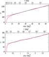 |
Fig. 11. Cumulative number of stars as a funcion of the distance to the cluster centre for NGC 2546A (up) and NGC 2546B (bottom). The upper abscissa axis is the distance to the cluster center and the lower abscissa axis the area of the corresponding circle. |
The cluster NGC 2546A extends up to almost r = 2 deg, with a half number radius of 28′. NGC 2546B is much smaller (half number radius of only 4′) and is completely superimposed to NGC 2546A, since the separation of their centres is about 17′. The total number of cluster stars was calculated by a linear fit of the cumulative number of stars as a function of the circle area (Eq. (1)). The main astrometric parameters are listed in Table 6: coordinates, proper motion, parallax, true distance modulus (from parallax), half number radius, and total number of stars brighter than G = 18 mag. We note that this approach to calculate the total number of cluster stars and half-mass radius is non-parametric and is free of any assumption on the radial distribution of cluster stars.
Lindoff (1968) found that the star distribution of NGC 2546 was not symmetrical, showing an elongated shape. We confirmed this fact and noted that this preferential direction coincides with the galactic plane. The ratio between the semi-minor and semi-major axis of the star distribution is about 0.6. Figure 12 shows density profiles measured in 2 deg wide strips along and perpendicular to the galactic equator.
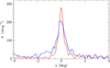 |
Fig. 12. Star density profiles of NGC 2546A along the direction of the galactic equator (blue) and perpendicular to it (red). |
5.2. Photometric distance and age
Gaia photometric data allow also to check the distance and estimate the age from the color–magnitude diagram. We used isochrones for Gaia photometric bands (Weiler 2018) corresponding to PARSEC stellar models (Bressan et al. 2012) for solar abundances, and isochrones of the MIST grid (Choi et al. 2016), corresponding to MESA stellar models (Paxton et al. 2011). Figure 13 shows the G vs. (GBP − GRP) color–magnitude diagram of probable members of the two clusters. From the spectral line width (see Table 1) we estimate that v sin i values for bright stars in both clusters cover evenly the range 0−300 km s−1. Therefore, MIST isochrones with stellar rotation (rotational velocity 0.4 times the critical value) are expected to be more appropriate. In left panel of Fig. 13 we have plotted for NGC 2546A three isochrones for the same age: PARSEC, MIST with rotation, and MIST without rotation. The differences are small and do not have much impact on the derived stellar parameters.
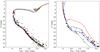 |
Fig. 13. Color–magnitude diagram of NGC 2546A (left) and NGC 2546B (right). In both cases only stars with proper motion and parallax consistent with the cluster have been plotted. In the left panel filled (open) symbols are stars with angular distance to the cluster centre in the range 0.0–0.4 deg (0.4–1.0 deg). Spectroscopic binaries are marked with open squares. Three isochrones for log τ = 8.25 are shown: PARSEC (green), MIST without rotation (blue), and MIST with rotation (red). In the right panel MIST isochrones (with rotation) for log τ = 6.0 (red), 6.7 (black), and 7.0 (blue) are plotted. Dashed line is the zero-age main-sequence. |
The color–magnitude diagram of NGC 2546A is very well fit by an isochrone of log(τ) = 8.25. The two SB2 (stars 10 and 30) and the RV variable (star 134) detected are close to the turn-off point. In the case of NGC 2546B the distance modulus is not well defined by the photometric data. We therefore adopted the distance modulus value derived from parallax. The interstellar absorption was calculated from the reddening, adopting AG/E(GBP − GRP) = 2.0 (Andrae et al. 2018). NGC 2546B is a very young cluster with about 80 members with G < 18 mag. Stars brighter than G ≈ 13 mag are main-sequence stars with masses higher than 2.5 M⊙. Below this limit, stars are still in the pre-main sequence stage, indicating an age below 10 Myr. In the Table 6 we present a summary of the parameters obtained for these two clusters, including half-number radius, distance modulus, and age.
6. Mixture model approach to cluster membership
In the previous sections we were able to detect the existence of two stellar clusters by analysing different observational data, among which RV and reddening were crucial. A relevant question is whether this result could have been obtained from Gaia data by an unsupervised learning method like Gaussian mixture models (GMM). As an experiment, we applied GMM to a star sample consisting of 56 000 Gaia sources brighter than G = 16 mag, within a 2 deg radius circle, and having all five astrometric parameters. The proper modeling of field star distribution required a large number of Gaussian components. This is not unexpected but a frequent result when all star data are included in a highly contaminated region (see for example Hosek et al. 2015; Olivares et al. 2018). The main reason is that the parameter distributions for the field are usually not Gaussian (Cabrera-Cano & Alfaro 1990; Sánchez & Alfaro 2009). Clearly the parallax distribution is intrinsically asymmetric (see Fig. 9) and the width of the proper motion distribution is a function of the distance (distant stars have small proper motion dispersion), to mention two obvious examples. Even considering up to 18 Gaussian components, we found difficult to detect both clusters with GMM. The most populous cluster NGC 2546A is easily detected but GMM fails to detect the small cluster NGC 2546B, unless a more limited input sample is defined trimming the variable domain to smaller ranges around the cluster position.
Besides the problem of non-Gaussian parameter distributions, we emphasize that the apparent magnitude distribution must be included in the calculation membership probabilities, since the level of field star contamination depends strongly on the magnitude. Even though very often cluster membership studies rely solely on proper motions, ignoring magnitudes or spatial position leads to a bias in membership probabilities, as was already noted by Francic (1989). In our approach we performed the GMM analysis with the five astrometric parameters, but calculated a posteriori membership probabilities taking into account the apparent magnitude distribution, by replacing the mixture weights by functions ϕ(G) representing the magnitude distribution of each mixture component. The cluster parameters, calculated by averaging all stars weighted with the membership probability, are entirely consistent with those consigned in Table 6. The color–magnitude diagram for all stars brighter than G = 17 mag in a 2 deg circle is shown in Fig. 14, where membership probability is indicated by the color scale. Only 357 out of a total of 115 350 stars have membership probability larger than 50%.
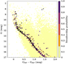 |
Fig. 14. Color–magnitude diagram of NGC 2546A, discriminating stars according to cluster membership probability. |
The high contamination level for faint magnitudes is illustrated in Fig. 15, which shows the fraction of member stars in a 0.2 deg circle centred in NGC 2546A as a function of apparent magnitude. At the cluster center about half of the bright stars are cluster members, while this fraction is reduced to 10% and for G = 14 mag and to only 1.4% for G = 17 mag.
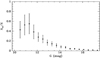 |
Fig. 15. Fraction of member stars as a function of apparent magnitude at the center of NGC 2546A. |
7. Discussion
We performed the first spectroscopic study of the cluster NGC 2546, determining spectral types and radial velocities for 28 probable cluster members. As a result, we detected three new spectroscopic binaries and distinguished two different stellar groups, superimposed in the sky but with a distance difference of about 500 pc. The identification of these two clusters was confirmed by a multicriteria membership analysis that included interstellar reddening, spectroscopic distance modulus, proper motion, and parallax. We determined the parameters of both clusters on the basis of our spectroscopic data, UBV photoelectric photometry from different sources, and Gaia astrometric and photometric data. This work shows how productive is to combine data obtained through different observational techniques to perform a comprehensive analysis of a system of interest. In particular, this paper, alike a number of recent studies of open clusters (e.g., Dias et al. 2018; Fritzewski et al. 2019), demonstrates the great usefulness of the precise Gaia data to determine age and distance of stellar clusters with scarce available information, as well as to obtain a better picture of their spatial dimension and structure.
Radial velocities, spectral types, and reddening were key to the detection of the duplicity of this cluster, particularly to the identification of NGC 2546B. Experiments with GMM applied to astrometric Gaia data in wide (1–2 deg) regions failed to detect the small cluster NGC 2546B. Besides the problems of non-Gaussian parameter distribution that affect the applicability of the standard GMM method and the need of a consistent inclusion of photometric magnitude distributions, reliable membership calculations must consider individual observational errors, which dominates the observed cluster dispersion. This kind of membership studies in the region of NGC 2546 would imply a complex mixture analysis (like in Olivares et al. 2018, for example), involving a large number of objects (in the field of NGC 2546 there are about 2.2 × 10⁵Gaia sources with r < 2 deg and G < 18 mag), which is beyond the scope of the paper, since the primary purpose of our astrometric analysis was to confirm the existence of two clusters and verify the membership of the observed stars.
The reddening and distance found by Lindoff (1968) agree with the values determined by us for NGC 2546A. The same holds for the parameters adopted in the catalogs of Dias et al. (2002), Joshi et al. (2016), and Loktin & Popova (2017), which are in the ranges d = 903−935 pc and E(B − V) = 0.13−0.15 mag. Nonetheless, the ages determined by previous works spread between our values for the clusters NGC 2546A and NGC 2546B: Lindoff (1968) estimated an age of 30 Myr, the catalogs of Dias et al. (2002) and Loktin & Popova (2017) adopted 74 Myr, and Joshi et al. (2016), 136 Myr.
There is no previous kinematic study of the cluster but the RV of the two red giants of NGC 2546A have been measured by Mermilliod et al. (2008) and by the Gaia mission. In both cases our results are in agreement with those works, being the mean differences 0.7 km s−1 with respect to Mermilliod et al. (2008) and less than 0.1 km s−1 with respect to Gaia.
The stellar content of NGC 2546A offers interesting cases for the study of the origin of spectroscopic peculiarities. We have detected two spectroscopic binaries with chemically peculiar components close to turn-off point. Using the mass ratio and the location in the color–magnitude diagram of these binaries we estimated masses for their components. The binary star 30 has a B7III primary with a mass of about 4.0 M⊙, which is at the end of the main-sequence, and a silicon secondary star with a mass of about 2 M⊙. The binary star 10, formed by two HgMn companions, has a primary of about 3.7 M⊙ that has already spent 85% of its main-sequence lifetime. These binaries share the turn-off region with other likely single, chemically normal stars (e.g., stars 165, 448, 353), and with the RV variable 134, that would be a long period binary with a chemically normal primary. From its location in the color–magnitude diagram we estimate that the primary of the binary 134 has a mass of about 3.8–3.9 M⊙ and has about 5% left of its main-sequence lifetime. Since all these stars have very similar masses and presumably the same age and original composition, the factors determining the occurrence of atmospheric chemical diffusion has to be found in the original rotational velocity, magnetic field, and binarity. The HgMn binary has an orbital period short enough for tidal forces to have effect on the rotational velocities. By contrast, in the binary with a silicon secondary, the physical properties of the stars would not be affected by the companion, since the orbital semiaxis is about 1100 R⊙.
Therefore, binaries with primaries of similar mass and evolutionary state can develop different chemical pattern in their atmospheres. In particularly, HgMn stars are often found in systems with periods between 3 and 20 days (Schöller et al. 2010), range in which stellar rotation, locked by tides, is slowed down. Our spectral resolution does not allow a reliable measure of projected stellar rotation, however, the spectral line broadening of the components of star 10 would suggests v sin i values on the order of 30–40 km s−1. This is consistent with co-rotation since, according to estimated masses and radii, the expected values of v sin i for pseudo-synchronization are 45 km s−1 and 32 km s−1 for the primary and secondary components.
Besides the binaries detected among the brightest stars of the cluster, another interesting fact of the color–magnitude diagram of NGC 2546A is that a sequence of binary stars with mass-ratio close to one would be perceptible in the lower main-sequence (Fig. 13).
The components of the two binaries (stars 257 and 475) and the RV variable (star 277) detected in the cluster NGC 2546B seem to be normal early B-type stars. The primaries of these systems are unevolved main-sequence stars. Considering their locations in the color–magnitude diagram and the mass-ratio, we estimated for the binary 257 stellar masses of about 9 and 7 M⊙. The orbit would have a semiaxis of ∼50 R⊙ and a low inclination angle (i ∼ 25°). The primary of the binary 475, would be one of the most massive stars of the cluster, with a mass on the order of 15 M⊙.
NGC 2546A is large and populous enough to discuss mass segregation within the cluster. Recomputing the calculations of the half-number radius in three magnitude ranges we obtain: R0.5 = 0.34 deg for G < 12 mag (corresponding to M ≳ 2 M⊙), R0.5 = 0.49 deg for G = 12−15 mag (2 M⊙ ≳ M ≳ 1 M⊙), and R0.5 = 0.68 deg for G = 15−18 mag (1 M⊙ ≳ M ≳ 0.6 M⊙). It is worth noting that the spectroscopic binaries 10, 30, and 134 are all three within a distance of only 0.13 deg from the cluster center.
Acknowledgments
Authors thank the support of CONICET through grant PIP 0331 and the Universidad Nacional de San Juan (Proyectos CICITCA and PROJOVI), Argentina. This research has made use of the WEBDA database, operated at the Department of Theoretical Physics and Astrophysics of the Masaryk University. This work has made use of data from the European Space Agency (ESA) mission Gaia (https://www.cosmos.esa.int/gaia), processed by the Gaia Data Processing and Analysis Consortium (DPAC, https://www.cosmos.esa.int/web/gaia/dpac/consortium). Funding for the DPAC has been provided by national institutions, in particular the institutions participating in the Gaia Multilateral Agreement.
References
- Andrae, R., Fouesneau, M., Creevey, O., et al. 2018, A&A, 616, A8 [NASA ADS] [CrossRef] [EDP Sciences] [Google Scholar]
- Arenou, F., Luri, X., Babusiaux, C., et al. 2018, A&A, 616, A17 [Google Scholar]
- Bertone, E., Buzzoni, A., Chávez, M., & Rodríguez-Merino, L. H. 2008, A&A, 485, 823 [NASA ADS] [CrossRef] [EDP Sciences] [Google Scholar]
- Bessell, M. S. 2000, PASP, 112, 961 [NASA ADS] [CrossRef] [Google Scholar]
- Bressan, A., Marigo, P., Girardi, L., et al. 2012, MNRAS, 427, 127 [NASA ADS] [CrossRef] [Google Scholar]
- Cabrera-Cano, J., & Alfaro, E. J. 1990, A&A, 235, 94 [NASA ADS] [Google Scholar]
- Cantat-Gaudin, T., Vallenari, A., Sordo, R., et al. 2018, A&A, 615, A49 [NASA ADS] [CrossRef] [EDP Sciences] [Google Scholar]
- Choi, J., Dotter, A., Conroy, C., et al. 2016, ApJ, 823, 102 [NASA ADS] [CrossRef] [Google Scholar]
- Claria, J. J. 1985, A&AS, 59, 195 [NASA ADS] [Google Scholar]
- Dias, W. S., Alessi, B. S., Moitinho, A., & Lépine, J. R. D. 2002, A&A, 389, 871 [NASA ADS] [CrossRef] [EDP Sciences] [Google Scholar]
- Dias, W. S., Monteiro, H., Lépine, J. R. D., et al. 2018, MNRAS, 481, 3887 [NASA ADS] [CrossRef] [Google Scholar]
- Duchêne, G., & Kraus, A. 2013, ARA&A, 51, 269 [Google Scholar]
- Francic, S. P. 1989, AJ, 98, 888 [NASA ADS] [CrossRef] [Google Scholar]
- Fritzewski, D. J., Barnes, S. A., James, D. J., et al. 2019, A&A, 622, A110 [NASA ADS] [CrossRef] [EDP Sciences] [Google Scholar]
- Gaia Collaboration (Brown, A. G. A., et al.) 2018a, A&A, 616, A1 [NASA ADS] [CrossRef] [EDP Sciences] [Google Scholar]
- Gaia Collaboration (Helmi, A., et al.) 2018b, A&A, 616, A12 [NASA ADS] [CrossRef] [EDP Sciences] [Google Scholar]
- González, E. J., & González, J. F. 2012, in Second Conference on Stellar Astrophysics, eds. J. A. Ahumada, M. C. Parisi, & O. I. Pintado, 126 [Google Scholar]
- González, J. F., & Lapasset, E. 2000, AJ, 119, 2296 [NASA ADS] [CrossRef] [Google Scholar]
- González, J. F., & Levato, H. 2006, A&A, 448, 283 [NASA ADS] [CrossRef] [EDP Sciences] [Google Scholar]
- Gray, R. O., Corbally, C. J., & Burgasser, A. J. 2009, Stellar Spectral Classification (Princeton: Princeton University Press) [Google Scholar]
- Harris, G. L. H. 1976, ApJS, 30, 451 [NASA ADS] [CrossRef] [Google Scholar]
- Hosek, Jr., M. W., Lu, J. R., Anderson, J., et al. 2015, ApJ, 813, 27 [NASA ADS] [CrossRef] [Google Scholar]
- Houk, N. 1982, Michigan Catalogue of Two-dimensional Spectral Types for the HD Stars. Volume 3. Declinations −40°.0 to −26°.0 [Google Scholar]
- Jaschek, C., & Jaschek, M. 2009, The Behavior of Chemical Elements in Stars (Cambridge: Cambridge University Press) [Google Scholar]
- Johnson, H. L., & Morgan, W. W. 1953, ApJ, 117, 313 [NASA ADS] [CrossRef] [Google Scholar]
- Joshi, Y. C., Dambis, A. K., Pandey, A. K., & Joshi, S. 2016, A&A, 593, A116 [NASA ADS] [CrossRef] [EDP Sciences] [Google Scholar]
- Leigh, N., & Geller, A. M. 2012, MNRAS, 425, 2369 [NASA ADS] [CrossRef] [Google Scholar]
- Leigh, N. W. C., & Geller, A. M. 2013, MNRAS, 432, 2474 [NASA ADS] [CrossRef] [Google Scholar]
- Lindegren, L., Hernández, J., Bombrun, A., et al. 2018, A&A, 616, A2 [NASA ADS] [CrossRef] [EDP Sciences] [Google Scholar]
- Lindoff, U. 1968, Arkiv Astron., 5, 63 [NASA ADS] [Google Scholar]
- Lodén, L. O. 1969, Arkiv Astron., 5, 149 [NASA ADS] [Google Scholar]
- Loktin, A. V., & Popova, M. E. 2017, Astrophys. Bull., 72, 257 [NASA ADS] [CrossRef] [Google Scholar]
- Luri, X., Brown, A. G. A., Sarro, L. M., et al. 2018, A&A, 616, A9 [NASA ADS] [CrossRef] [EDP Sciences] [Google Scholar]
- Maitzen, H. M. 1982, A&A, 115, 275 [NASA ADS] [Google Scholar]
- Mermilliod, J. C., Mayor, M., & Udry, S. 2008, A&A, 485, 303 [NASA ADS] [CrossRef] [EDP Sciences] [Google Scholar]
- Olivares, J., Sarro, L. M., Moraux, E., et al. 2018, A&A, 617, A15 [NASA ADS] [CrossRef] [EDP Sciences] [Google Scholar]
- Paxton, B., Bildsten, L., Dotter, A., et al. 2011, ApJS, 192, 3 [Google Scholar]
- Piskunov, A. E., Schilbach, E., Kharchenko, N. V., Röser, S., & Scholz, R. D. 2007, A&A, 468, 151 [NASA ADS] [CrossRef] [EDP Sciences] [Google Scholar]
- Sánchez, N., & Alfaro, E. J. 2009, ApJ, 696, 2086 [NASA ADS] [CrossRef] [Google Scholar]
- Schild, R. E., Garrison, R. F., & Hiltner, W. A. 1983, ApJS, 51, 321 [NASA ADS] [CrossRef] [Google Scholar]
- Schmidt-Kaler, T. 1982, in Landolt-Bornstein, New Series, Group VI, eds. K. Schaifers, & H. H. Voigt (Berlin: Springer), 2b [Google Scholar]
- Schöller, M., Correia, S., Hubrig, S., & Ageorges, N. 2010, A&A, 522, A85 [NASA ADS] [CrossRef] [EDP Sciences] [Google Scholar]
- Sota, A., Maíz Apellániz, J., Morrell, N. I., et al. 2014, ApJS, 211, 10 [NASA ADS] [CrossRef] [Google Scholar]
- Vasiliev, E. 2019, MNRAS, 489, 623 [NASA ADS] [CrossRef] [Google Scholar]
- Weiler, M. 2018, A&A, 617, A138 [NASA ADS] [CrossRef] [EDP Sciences] [Google Scholar]
All Tables
All Figures
|
Fig. 1. Spectral separation of the SB2s 30 (right panel) and 257 (left panel). Two observed spectra taken at different orbital phases are plotted for each star. The reconstructed spectra of the two stellar component are shown in blue and red. Below, in thin black line, is the spectrum modeled combining the two spectra of the components, and below it, in heavy black line, the observed spectrum. |
| In the text | |
|
Fig. 2. Radial velocity curves of the four studied binaries: NGC 2546−10 (upper left), NGC 2546−30 (upper right), NGC 2546−257 (lower left), and NGC 2546−475 (lower right). |
| In the text | |
|
Fig. 3. RV distribution of observed objects. Each star is represented by a Gaussian whose width depends on the RV error. Heavy black line is the global RV distribution. Blue and red lines show the distributions of stars classified as members of the clusters NGC 2546A and NGC 2546B, respectively. |
| In the text | |
|
Fig. 4. Color–color diagram obtained with the available photoelectric photometry and the standard sequence of Schmidt-Kaler (1982). The dashed line corresponds to E(B − V) = 0.00, the black and gray continuous lines correspond to E(B − V) = 0.14 mag and E(B − V) = 0.29 mag respectively. |
| In the text | |
|
Fig. 5. Spectroscopic reddening and distance modulus. Filled circles are stars with photoelectric photometry. Blue, red, and green symbols are stars belonging to NGC 2546A, NGC 2546B, and the galactic field, respectively, according to our multicriteria final assignment. Open triangles correspond to Tycho magnitudes (see text). |
| In the text | |
|
Fig. 6. Proper motion of RV members of the two clusters. Blue circles are RV members of NGC 2546A; filled circles are stars with RV uncertainties below 1.1 km s−1. Red diamonds are RV members of NGC 2546B; the filled red square is the O-type star 682. The other stars are Gaia sources with magnitude G < 14 mag. |
| In the text | |
|
Fig. 7. Proper motion distribution of Gaia stars brighter than G = 14 mag. The position of clusters NGC 2546A and NGC 2546B are at the intersection of continuous red lines and dashed blue lines, respectively. |
| In the text | |
|
Fig. 8. Sections of the proper motion distribution along the vertical and horizontal lines shown in Fig. 7. Upper panels correspond to NGC 2546A and lower panels to NGC 2546B. |
| In the text | |
|
Fig. 9. Parallax distribution of stars within a circle of 1 deg radius. Upper panel: stars brighter than G = 14 mag. Vertical lines mark the position of the two clusters. Middle panel: stars brighter than G = 16 mag with proper motion consistent with the cluster NGC 2546A. Lower panel: stars brighter than G = 16 mag with proper motion consistent with NGC 2546B in a circle of 1 deg radius (red curve) and in a 0.1 deg radius circle centred in the coordinates of NGC 2546B (gray filled curve). |
| In the text | |
|
Fig. 10. Spatial distribution of stars with G < 16 mag and proper motion compatible with the cluster NGC 2546B. |
| In the text | |
|
Fig. 11. Cumulative number of stars as a funcion of the distance to the cluster centre for NGC 2546A (up) and NGC 2546B (bottom). The upper abscissa axis is the distance to the cluster center and the lower abscissa axis the area of the corresponding circle. |
| In the text | |
|
Fig. 12. Star density profiles of NGC 2546A along the direction of the galactic equator (blue) and perpendicular to it (red). |
| In the text | |
|
Fig. 13. Color–magnitude diagram of NGC 2546A (left) and NGC 2546B (right). In both cases only stars with proper motion and parallax consistent with the cluster have been plotted. In the left panel filled (open) symbols are stars with angular distance to the cluster centre in the range 0.0–0.4 deg (0.4–1.0 deg). Spectroscopic binaries are marked with open squares. Three isochrones for log τ = 8.25 are shown: PARSEC (green), MIST without rotation (blue), and MIST with rotation (red). In the right panel MIST isochrones (with rotation) for log τ = 6.0 (red), 6.7 (black), and 7.0 (blue) are plotted. Dashed line is the zero-age main-sequence. |
| In the text | |
|
Fig. 14. Color–magnitude diagram of NGC 2546A, discriminating stars according to cluster membership probability. |
| In the text | |
|
Fig. 15. Fraction of member stars as a function of apparent magnitude at the center of NGC 2546A. |
| In the text | |
Current usage metrics show cumulative count of Article Views (full-text article views including HTML views, PDF and ePub downloads, according to the available data) and Abstracts Views on Vision4Press platform.
Data correspond to usage on the plateform after 2015. The current usage metrics is available 48-96 hours after online publication and is updated daily on week days.
Initial download of the metrics may take a while.