| Issue |
A&A
Volume 633, January 2020
|
|
|---|---|---|
| Article Number | A129 | |
| Number of page(s) | 7 | |
| Section | Galactic structure, stellar clusters and populations | |
| DOI | https://doi.org/10.1051/0004-6361/201935833 | |
| Published online | 22 January 2020 | |
ESPRESSO highlights the binary nature of the ultra-metal-poor giant HE 0107−5240⋆
1
GEPI, Observatoire de Paris, Université PSL, CNRS, 5 Place Jules Janssen, 92190 Meudon, France
e-mail: This email address is being protected from spambots. You need JavaScript enabled to view it.
, This email address is being protected from spambots. You need JavaScript enabled to view it.
2
Istituto Nazionale di Astrofisica, Osservatorio Astronomico di Trieste, Via G.B. Tiepolo 11, 34143 Trieste, Italy
3
Institute for Fundamental Physics of the Universe, Via Beirut, 2, 34151 Grignano, Trieste, Italy
4
Instituto de Astrofísica e Ciências do Espaço, Universidade do Porto, CAUP, Rua das Estrelas, 4150-762 Porto, Portugal
5
Institute of Astronomy, University of Cambridge, Madingley Rd, Cambridge CB3 0HA, UK
6
Physikalisches Institut, Universität Bern, Bern, Switzerland
7
Instituto de Astrofísica de Canarias, Vía Láctea, 38205 La Laguna, Tenerife, Spain
8
Scuola Normale Superiore, P.zza dei Cavalieri 7, 56126 Pisa, Italy
9
Universidad de La Laguna, Departamento de Astrofísica, 38206 La Laguna, Tenerife, Spain
10
Observatoire de l’Université de Genève, Ch. des Maillettes 51, 1290 Versoix, Switzerland
11
European Southern Observatory, Casilla 19001, Santiago, Chile
12
Centro de Astrofísica da Universidade do Porto, Rua das Estrelas, 4150-762 Porto, Portugal
13
Istituto Nazionale di Astrofisica, Osservatorio Astronomico di Palermo, Piazza del Parlamento 1, Palermo, Italy
14
Departamento de Ciencias Fisicas, Universidad Andres Bello, Fernandez Concha 700, Las Condes, Santiago, Chile
15
Instituto de Astrofísica e Ciências do Espaço, Faculdade de Ciências da Universidade de Lisboa, Campo Grande, Lisboa 1749-016, Portugal
16
Istituto Nazionale di Astrofisica, Osservatorio Astronomico di Brera, Via E. Bianchi 46, 23807 Merate, LC, Italy
17
Fundación Galileo Galilei – INAF, Rambla José Ana Fernandez Pérez 7, 38712 Breña Baja, Spain
18
Departamento de Física e Astronomia, Faculdade de Ciências, Universidade do Porto, Rua do Campo Alegre, 4169-007 Porto, Portugal
19
Istituto Nazionale di Astrofisica, Osservatorio Astrofisico di Torino, Via Osservatorio 20, 10025 Pino Torinese, Italy
20
Centro de Astrobiología (CSIC-INTA), Carretera Ajalvir km 4, 28850 Torrejón de Ardoz, Madrid, Spain
Received:
3
May
2019
Accepted:
4
July
2019
Abstract
Context. The vast majority of the known stars of ultra low metallicity ([Fe/H] < −4.5) are known to be enhanced in carbon, and belong to the “low-carbon band” (A(C) = log(C/H)+12 ≤ 7.6). It is generally, although not universally, accepted that this peculiar chemical composition reflects the chemical composition of the gas cloud out of which these stars were formed. The first ultra-metal-poor star discovered, HE 0107−5240, is also enhanced in carbon and belongs to the “low-carbon band”. It has recently been claimed to be a long-period binary, based on radial velocity measurements. It has also been claimed that this binarity may explain its peculiar composition as being due to mass transfer from a former AGB companion. Theoretically, low-mass ratios in binary systems are much more favoured amongst Pop III stars than they are amongst solar-metallicity stars. Any constraint on the mass ratio of a system of such low metallicity would shed light on the star formation mechanisms in this metallicity regime.
Aims. We acquired one high precision spectrum with ESPRESSO in order to check the reality of the radial velocity variations. In addition we analysed all the spectra of this star in the ESO archive obtained with UVES to have a set of homogenously measured radial velocities.
Methods. The radial velocities were measured using cross correlation against a synthetic spectrum template. Due to the weakness of metallic lines in this star, the signal comes only from the CH molecular lines of the G-band.
Results. The measurement obtained in 2018 from an ESPRESSO spectrum demonstrates unambiguously that the radial velocity of HE 0107−5240 has increased from 2001 to 2018. Closer inspection of the measurements based on UVES spectra in the interval 2001–2006 show that there is a 96% probability that the radial velocity correlates with time, hence the radial velocity variations can already be suspected from the UVES spectra alone.
Conclusions. We confirm the earlier claims of radial velocity variations in HE 0107−5240. The simplest explanation of such variations is that the star is indeed in a binary system with a long period. The nature of the companion is unconstrained and we consider it is equally probable that it is an unevolved companion or a white dwarf. Continued monitoring of the radial velocities of this star is strongly encouraged.
Key words: binaries: spectroscopic / stars: abundances / Galaxy: abundances / Galaxy: halo
Tables 1 and 2 are also available at the CDS via anonymous ftp to cdsarc.u-strasbg.fr (130.79.128.5) or via http://cdsarc.u-strasbg.fr/viz-bin/cat/J/A+A/633/A129
© P. Bonifacio et al. 2020
 Open Access article, published by EDP Sciences, under the terms of the Creative Commons Attribution License (http://creativecommons.org/licenses/by/4.0), which permits unrestricted use, distribution, and reproduction in any medium, provided the original work is properly cited.
1. Introduction
The ultra-metal-poor star HE 0107−5240 was the first star that was discovered to have [Fe/H]1 < − 5.0 (Christlieb et al. 2002). Its chemical composition departs significantly from what was, at the time, considered the standard composition of extremely metal-poor stars. That is, for stars in which most elements are solar-scaled, with an enhancement of α elements over iron and a large scatter in the abundances of neutron capture elements (Bessell & Norris 1984; Molaro & Castelli 1990; Molaro & Bonifacio 1990; Primas et al. 1994; McWilliam et al. 1995; Ryan et al. 1996; Spite et al. 2000). Instead it was clear from the beginning that HE 0107−5240 belonged to the class of carbon-enhanced, metal-poor stars (Barbuy et al. 1997; Norris et al. 1997a). At the time most such stars appeared to be enhanced in neutron capture elements and their peculiar chemical composition was thought to be the result of mass transfer from an Asymptotic Giant Branch (AGB) companion, in fact being the extremely-metal-poor counterpart of CH stars (Vanture 1992a,b; McClure 1997). The discovery of CS 22957−27 (Norris et al. 1997b; Bonifacio et al. 1998) led to the introduction of a new class of stars that is carbon enhanced, but not enhanced in neutron capture elements. In turn this led to a questioning of the universality of the mass-transfer scenario for carbon-enhanced metal-poor stars; this class is currently known as CEMP-no (Beers & Christlieb 2005). HE 0107−5240 appeared immediately to be not enhanced in neutron capture elements and therefore in the same class as CS 22957−27, although two orders of magnitude lower in [Fe/H].
It was already well appreciated how difficult, or even impossible, it is to form a low-mass star from metal-free gas. In his review, Palla (2003) describes the current knowledge on primordial star formation at the time, as well as the surprise of finding a star as poor in [Fe/H] as HE 0107−5240. The majority of the community started to work on the hypothesis that the chemical composition of HE 0107−5240 reflects the composition of the gas out of which it was formed and was the result of enrichment by one or several supernovae (SNe; Umeda & Nomoto 2003; Bonifacio et al. 2003; Limongi et al. 2003). Also the formation of low-mass stars from such gas was explored (Schneider et al. 2003). In a very influential paper, Bromm & Loeb (2003) developed a theory showing how atomic lines of neutral oxygen and singly ionised carbon could effectively cool a metal-poor contracting cloud, provided the abundance of these elements was high enough. In the following years, other ultra-metal-poor stars were found (Frebel et al. 2005; Norris et al. 2007) and they were all carbon enhanced like HE 0107−5240. This led to the idea that all ultra-metal-poor stars were necessarily carbon enhanced. It was not until recently that ultra-metal-poor stars that are not carbon enhanced have been found (Caffau et al. 2011; Starkenburg et al. 2018), implying that metal-line cooling is not the only mechanism capable of allowing the formation of a low-mass, ultra-metal-poor star.
At the time of writing there are 14 stars known to have [Fe/H] < −4.5, and they are listed in Table 1. All of the 12 carbon-enhanced stars lie on the low-carbon band defined by Bonifacio et al. (2018). All of the stars on the low-carbon band for which it has been possible to assess the abundances of n-capture elements classify them as CEMP-no. This is a clear difference with the high-carbon band stars, which are almost all enhanced in s-process elements and classified as CEMP-s. Furthermore, the observations of Lucatello et al. (2005) and Starkenburg et al. (2014) have given a strong indication that CEMP-s stars are likely to be all binary stars. The high-carbon band stars are generally considered to be the result of mass transfer from a former AGB companion (Bonifacio et al. 2015, 2018), while the low-carbon band stars are generally considered to reflect the chemical composition of the gas cloud out of which they were formed.
Stars with [Fe/H] < −4.5.
In spite of the fact that the majority of the community accepted the chemical composition of HE 0107−5240, and its siblings, as being the same as that of the gas clouds out of which they formed, dissenting opinions that invoke mass transfer from a companion exist (Suda et al. 2004; Lau et al. 2007; Cruz et al. 2013). Such models are compatible with the observed lack of enhancement in n-capture elements. For HE 0107−5240 this possibility was often discarded because of the lack of any variation in its radial velocity over an interval of five years (2001–2006).
In the meanwhile, Arentsen et al. (2019) presented some low quality radial velocity measurements obtained with the High Resolution Spectrograph (Bramall et al. 2012) on the Southern African Large Telescope (SALT; Buckley et al. 2006). In spite of the large errors on their four measurements, the indication was clear that the radial velocity of HE 0107−5240 was almost 4 km s−1 larger than it was in the time interval 2001–2006. On this basis, Arentsen et al. (2019) suggested that the scenario of mass transfer in this star becomes highly likely. We note that mass transfer can also occur in a very wide binary, if it happens mainly through the stellar wind (Abate et al. 2018).
Since HE 0107−5240 is a prototype of the ultra-metal-poor, carbon-enhanced stars and so much effort has gone into the interpretation of its chemical abundances, we decided to observe it with the Echelle SPectrograph for Rocky Exoplanets and Stable Spectroscopic Observations (ESPRESSO; Pepe et al. 2013) in GTO time to look for radial velocity variations. We also re-analysed the Ultraviolet and Visual Echelle Spectrograph (UVES; Dekker et al. 2000) spectra retrieved from the ESO archive.
2. Observations and radial velocity measurements
We observed HE 0107−5240 on September 3, 2018 with ESPRESSO in the high resolution (HR) mode. In this mode the light collected from a single unit telescope is channeled by a full-optics coudé train to the combined coudé laboratory. In the coudé laboratory the light is fed to a dedicated front-end sub-system (one for each Unit Telescope (UT) that may be used) and corrected for atmospheric dispersion. The front-end unit feeds the light to the optical fibres. In the HR mode there are two fibres with a core diameter of 140 μm that corresponds to 1 0 on the sky. We decided to use one fibre for the star and the second for the sky. Before entering the spectrograph the light passes through the Anamorphic Pupil Slicing Unit. This optical system allows the compression of the beam in the direction of the cross-dispersion and splits the beam into two slices. Thus in ESPRESSO observations each échelle order on the detector is composed of four slices, in our case two for the star and two for the sky. We used a CCD binning 2 × 1 (two in the spatial direction) and a slow read-out mode, which results in a read-out-noise of 3 e− pixel−1 in the blue CCD of the mosaic and 2 e− pixel−1 in the red CCD. The exposure time was 3300 s. The seeing was about 1
 5, significantly larger than the 1
 0 aperture on the sky of the ESPRESSO high resolution fibre mode, leading to a significant light loss. The spectra were reduced using the ESPRESSO pipeline version 1.2.32. The pipeline performs background subtraction using the inter-order pixels, an optimal extraction on each of the slices, and a flat-field correction on the extracted spectra. The wavelength solution was derived using the spectrum of a ThAr lamp combined with a Fabry-Pérot Etalon. The spectrum of the sky fibre was scaled to take into account the different transmission of the two fibres as estimated from flat-field spectra, rebinned to the same step as the star spectrum and finally subtracted. The wavelength solution was corrected for the barycentric radial velocity at the time of observation. Finally the slices were rebinned, combined, and the orders merged. The step of the rebinned spectrum is close to the size of the original pixels as read-out from the CCD; in our case, taking into account the on-chip binning, we have a mean pixel size of 0.7 pm3 in the region of the G-band. The spectrum so obtained was calibrated in absolute flux using an absolute efficiency curve, derived from observations of flux standard stars. This flux calibration is aimed at having a good relative flux, but cannot take into account either slit losses or atmospheric absorption at the time of observation. During the reduction steps the pipeline computes errors in the spectrum and propagates the errors due to read-out noise, dark current, photon noise (source plus background), flat-fielding, and sky subtractions. The propagation is straightforward up to the rebinning step to produce one-dimensional spectra. The rebinning introduces a correlation between pixels. The pipeline propagates the error to the rebinned spectrum, but also provides an additional array that provides a correlation factor of each pixel. In our analysis we ignored the correlation between pixels in the rebinned spectrum and used the error provided by the pipeline to estimate the achieved signal-to-noise ratio (S/N) per pixel. In the region 433.55–433.83 nm, we find ⟨S/N⟩ = 2.4.
We also retrieved all the spectra obtained with UVES in the period 2001–2006 with different settings and slit widths, providing resolving power between 41 000 and 66 000. We used all the blue-arm spectra that covered the G-band, using exactly the same wavelength interval used to measure the ESPRESSO spectrum and the same template, except that for UVES the template was broadened so as to match the resolution provided by the slit width of each UVES spectrum. We used also the red-arm spectra that covered the Mg I b triplet. We did not use any of the UV or IR UVES spectra.
To measure radial velocities we used cross correlation against a synthetic spectrum template. This was computed using an ATLAS 9 model (Kurucz 2005) with Teff = 5100 K, log g = 2.2, metallicity −5.0, a standard α element enhancement of 0.4 dex, and microturbulence of 1.0 km s−1. From this model we used the SYNTHE (Sbordone et al. 2004; Kurucz 2005) spectrum synthesis code to compute a spectrum with microturbulence 2.2 km s−1 and the abundances derived by Christlieb et al. (2004), except for the oxygen abundance, for which we adopted the value of Bessell et al. (2004). We verified by comparison with the UVES archive spectra that this synthetic spectrum provides a close match both to the G-band and for the Mg I b triplet.
For the ESPRESSO spectrum we did not get any signal from the region around the Mg I b triplet, but we did get a very strong and clear signal from the G-band as shown in Fig. 1. The cross correlation was computed in Fourier space (by Fast Fourier Transform) in the ln(λ) space, following Tonry & Davis (1979). The considered interval was 400–449.8 nm, the observed spectra were continuum subtracted so that the “continuum” appeared at zero. The same operation was done to the template spectrum, which was previously broadened to a resolving power of R = 140 000. The error was estimated from the width and contrast of the peak of the cross correlation function, as described in Tonry & Davis (1979). For the UVES blue-arm spectra, we estimated the error from the cross correlation function and added 0.5 km s−1 to this to account for the uncertainty on the centring of the star on the slit (Molaro et al. 2008). In addition we measured all the UVES red-arm spectra that contained the Mg I b triplet. Some of these were observed coupled with some of the above-mentioned blue-arm spectra, but others were coupled with the 346 nm blue-arm spectrum, which does not cover the G-band. Since the UVES spectra were all acquired with the purpose of determining chemical abundances they all have a high S/N ratio for radial velocity determination (S/N ≈ 40 or higher), the Mg I b triplet always provides a very good and clean signal. All of the red-arm spectra cover the O2 X0 − b2 band around 630 nm produced by the Earth’s atmosphere. In spite of the known changes in shape due to pressure changes in the atmosphere, the wavelength position of these lines is stable at the level of 10 m s−1 over six years (Figueira et al. 2010). Gettel (2012) also describe the use of telluric lines for high precision radial velocities. We used atmospheric transmission synthetic spectra computed by Transmissions Atmosphériques Personnalisées pour l’AStronomie (TAPAS; Bertaux et al. 2014) as a template over the range 623–655 nm. This range also includes some weaker H2O lines, which are less stable than the O2 lines. We cross correlated this template with the observed spectra and measured the radial velocity of the telluric lines; this radial velocity was subtracted from the observed radial velocity. A possible concern is that the radial velocity is measured from a portion of the spectrum extracted from the lower CCD of the red arm of UVES, while the position of the telluric lines is measured on a portion of spectrum extracted from the upper CCD. In the UVES data reduction pipeline, independent wavelength solutions are obtained for the two CCDs. Molaro et al. (2008) have shown that the two CCDs of UVES provide radial velocities that are consistent to better than 0.1 km s−1, which is well beyond the accuracy we can expect from our spectra. In principle the measurement of the tellurics corrects for the positioning of the star on the slit. We always found the shift of the tellurics to be less than 1 km s−1 and the error on this shift, estimated from cross correlation function, is always less than 0.2 km s−1. This error was added linearly to the error derived from the measurement of the Mg I b triplet to provide our total error estimate.
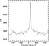 |
Fig. 1. Cross correlation function of ESPRESSO spectrum with the synthetic spectrum template. |
Applying these shifts reduces slightly the scatter in the radial velocity measurements, however, it should be stressed that none of the results discussed in the next section depend crucially on these corrections. The conclusion would be the same if we just take the observed velocities.
Some of our blue-arm spectra are coupled with red-arm spectra that contain the Mg I b triplet, namely four spectra in 2001, one in 2004, one in 2005, and one in 2006. For these spectra we explored the effect of applying the shift deduced from the tellurics in the red arm also to the velocity derived from the blue arm. The rationale for this is that if the slits of the two arms were perfectly aligned, then the shift measured in the red arm should also apply to the blue arm. Molaro et al. (2008) have shown that the radial velocities derived from the blue arm match those of the red arm to better than 0.1 km s−1 suggesting that the two slits are indeed well aligned. This result cannot, however, be generalised and in the lifetime of UVES the slits have been dismounted and re-aligned, because larger shifts between blue and red had been noticed. In our case the results of also applying the shift deduced from the red arm to the blue arm are not so clear. The success of the technique in the 2001 measurement is striking; the average red-blue goes from 0.267 km s−1 without correction to 0.047 km s−1 with correction of the blue spectra. However, for the 2004 spectra the red-blue difference goes from 0.772 km s−1 without correction to 0.963 km s−1 with correction. We therefore decided not to apply any correction to the blue spectra. Again we stress that none of our conclusions depend on this choice.
All of our measurements are summarised in Table 2. For the red arm spectra we also provide the velocity of the telluric lines and the error on that velocity. In Table 2 we report the four measurements of Arentsen et al. (2019).
Measured radial velocities of HE 0107−5240.
3. Discussion
3.1. Is the radial velocity of HE 0107−5240 variable or constant?
In Fig. 2 we provide all our measurements with the associated error bars and we also add the four data points of Arentsen et al. (2019). The measurements on the UVES data seem somewhat dispersed, however a non-parametric test to assess whether time and radial velocity are correlated provides a probability of correlation of 96%, both using Kendall’s τ and Spearman’s rank correlation. This means that even from the UVES data alone we should suspect that the star is a radial velocity variable. If then we add to the sample the measurement with ESPRESSO, this probability rises to 98.7%, at which point we can consider it certain that the radial velocity varies. The measurements of Arentsen et al. (2019) are less precise than the others, however they also support a variation of the radial velocity of HE 0107−5240. Since for a long time the radial velocity of HE 0107−5240 has been considered constant, based on the UVES spectra we should also ask the question: is it possible that the UVES measurements have a systematic error so that they are 3 km s−1 lower than the true value? As usual it is very difficult to exclude the presence of systematic errors in any given instrument. The first evidence against any systematic error is precisely the fact that a rank correlation provides a 96% probability of correlation, based on UVES data alone. Thus a higher radial velocity at later dates is indeed expected. If we applied a constant offset of 3 km s−1 to all the UVES data, the correlation would still be there and the fact that over ten years after the radial velocity is the same would be difficult to explain. The second argument against any systematic effect is that UVES is an instrument that is known to be both accurate and precise in radial velocity (e.g. Molaro et al. 2008) and systematic effects of this magnitude have never been reported. A third argument is that the measurements in the four different settings used (blue arm 390 nm and 437 nm; red arm 564 nm and 580 nm) are, by and large, consistent over a time span of five years. It is difficult to think of a systematic effect that would act in the same way for four different instrumental settings over such a long period of time. We conclude that the presence of systematic effects in the measurement of the UVES spectra at the level of 3 km s−1 is very unlikely.
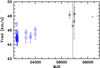 |
Fig. 2. Radial velocities of HE 0107−5240 as a function of time (MJD) of observation. Open symbols are our measurements on UVES spectra. Asterisks are the measurements of Arentsen et al. (2019). The small red dot is our measurement our measurements on the ESPRESSO spectrum. |
Let us check if the dispersion in the UVES measurements is compatible with the measurement errors. Since we know that there is a long-term trend in radial velocity, we isolate the measurements of 2001 (9 measurements) and 2002 (18 measurements); the standard deviation around the mean is 0.256 km s−1 for the 2001 measurements and 0.599 km s−1 for 2002. For 2001 the dispersion is much smaller than the mean measurement error. We can thus say that the dispersion is fully compatible with measurement errors. For the 2002 measurements the dispersion is slightly higher than the mean total error (0.425 km s−1). It is possible, although we cannot conclusively demonstrate it, that a part of this dispersion is due to the radial velocity jitter that is observed in some metal-poor red giants (Carney et al. 2003). This jitter can be as large as a few km s−1. To explain it, combinations of multiple causes have been invoked, including stellar oscillations, star spots, stellar activity, and stellar granulation. The majority of the stars that show radial velocity jitter are considerably more luminous than HE 0107−5240 (MV = –0.34, using the Gaia second data release (Gaia DR2; Gaia Collaboration 2018; Arenou et al. 2018, parallax of 0.079 mas), yet some stars of even lower luminosity are known to show some jitter (see Fig. 8 of Carney et al. 2003).
We consider the long-term radial velocity variation of HE 0107−5240 claimed by Arentsen et al. (2019) to be robustly confirmed by our measurements. The simplest explanation of such long-term variation is that HE 0107−5240 is in a binary system. Arentsen et al. (2019) computed plausible orbits and say that their orbit period distribution peaks in the interval 27–82 years. The time baseline did not allow us to obtain a reliable estimate of such a very long period. Moreover, just a trend, without a maximum or a minimum, was observed (Fig. 2). The amplitude spectrum of our data is shown in Fig. 3. The highest peak close to 0.0 is the unconstrained period due to the observed long trend; peaks at 0.5 and 1.0 d−1 are due to the spectral window. The mean level of the noise is 0.5 ± 0.3 km s−1. A significant peak should have S/N ≥ 4.0 (Kuschnig et al. 1997) but clearly none with an amplitude greater than 2.0 km s−1 stands out. Therefore, no periodicity smaller than the time span of the observations can be detected.
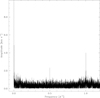 |
Fig. 3. Amplitude spectrum of HE 0107−5240 data. |
3.2. If HE 0107−5240 is a binary system, what is the nature of the less luminous companion?
Let us assume, for the sake of discussion, that HE 0107−5240 is indeed a binary system. The question arises as to the mass and the nature of the companion. Being a giant, HE 0107−5240 will outshine any unevolved companion or white dwarf companion at all wavelengths from vacuum ultraviolet to far infrared. The star is detected in Galex (Morrissey et al. 2005, 2007) NUV and not in the FUV filter (λeff = 213.6 nm and λeff = 153.9 nm, respectively Bianchi et al. 2011). The measured flux in the near-ultraviolet (NUV) band and lack of measurement in the far-ultraviolet (FUV) band is compatible with the theoretical flux distribution for HE 0107−5240. This is consistent with the findings of Venn et al. (2014) who explored the spectral energy distribution from 444 nm to 22 080 nm. They claimed a marginal detection of an IR excess in the Wide-Field Infrared Survey Explorer (WISE; Wright et al. 2010) W3 band (λeff = 11560 nm). The ALLWISE (Cutri et al. 2014) W3 photometry is about 0.3 mag fainter than that used in Venn et al. (2014), but since it is only at the level of a detection of 3.1σ, it is very difficult to detect an IR excess at this low S/N ratio. The spectral energy distribution of HE 0107−5240 cannot give us any hint as to the nature of the companion. Although it is possible that it is a white dwarf that in its AGB phase transferred mass to the currently observed giant, as advocated by Suda et al. (2004), Lau et al. (2007), Cruz et al. (2013), and Arentsen et al. (2019), it is equally probable that it is an unevolved star.
Further observations of HE 0107−5240 with high precision on the radial velocity may, in the future, allow us to determine the orbit of the system and its mass function4. The mass of the primary star (i.e. the star that is currently visible) can be estimated through the use of isochrones. This, coupled with an assumption of the orbit’s inclination, will provide an estimate of the mass of the secondary. This information may constrain the nature of the companion star. The mass distribution of white dwarfs is sharply peaked at about 0.55 M⊙ (Kepler et al. 2007). If we assume that the initial mass function (IMF) of the stars in the metallicity regime of HE 01507−5240 follows Kroupa’s law (Kroupa 2001, 2002), then we expect a peak at about 0.1 M⊙. If the mass estimated for the unseen companion is low, say 0.2 M⊙, one can reasonably argue that it is unlikely to be a white dwarf. However, if the mass is on the order of 0.5 M⊙, it is not possible to draw any firm conclusion, since the Kroupa IMF (and any other IMF) predicts a sizeable number of stars of this mass; unlike the mass distribution of white dwarfs, the peak is not sharp. The further complication is the uncertainty on the inclination of the orbit. While it is possible to make a statistical estimate of the most probable value of the inclination, it is impossible to rule out any value. Thus a low-mass estimate for the companion could simply result from a nearly edge-on orbit. Only if the binary motion could be observed in some other way (photometric, visual, astrometric) would it be possible to break the degeneracy and measure the orbit inclination. We note that in the Gaia DR2, HE 0107−5240 shows no excess astrometric noise.
3.3. Implications for the star formation processes at ultra-low metallicity
High resolution simulations of star formation from primordial gas have shown the importance of the fragmentation processes (Greif et al. 2011). On the one hand, this provides a way to produce low-mass stars even in the absence of efficient cooling mechanisms, on the other hand it may be a way to favour the formation of binary systems. In fact the simulations of Stacy & Bromm (2013) predict a binary fraction of 35% for Pop III stars and the period distribution is peaked at P ≲ 900 yr. According to Stacy & Bromm (2013), in Pop III stars low-mass ratios of the binary members are much more favoured than they are amongst solar-metallicity stars (Duquennoy & Mayor 1991). If one could measure the mass function of the system, this would place constraints on the mass of the secondary. This, in turn, could be used to constrain the nature of the secondary, using the theoretical distribution of mass ratios for primordial stars. One crucial point in the simulation of primordial star formation is to be able to follow the simulations long enough to understand how many of the fragments merge again and end up as massive stars, and how many end up as binary or multiple systems. This is computationally challenging and for the time being there is no consensus on the long-term evolution of the fragments.
Hartwig & Yoshida (2019) have suggested an interesting scenario in which the CEMP stars form as a consequence of inhomogeneous metal mixing. Although this scenario is appealing, it is not clear how it can be reconciled with the homogeneity of abundance ratios in low-carbon band stars for elements heavier than Si (Bonifacio et al. 2015) or with the homogeneity of all abundance ratios in carbon-normal stars (Cayrel et al. 2004; Bonifacio et al. 2009).
4. Conclusions
Thanks to the exquisite radial velocity precision of ESPRESSO, and the long baseline afforded by the ESO observations, we have confirmed the long-term variability in radial velocity of HE 0107−5240 claimed by Arentsen et al. (2019). The simplest explanation of this variability is that HE 0107−5240 is a long-period binary system. The current observations, however, do not provide any constraint on the nature of the companion that could be, with equal probability, a white dwarf or an unevolved star. Unfortunately this does not provide any progress on whether HE 0107−5240 has undergone mass transfer from an AGB companion or not. We encourage continued monitoring of the radial velocity of this system with high precision instruments.
[Fe/H] = log(Fe/H) – log(Fe/H)⊙.
The pipeline and its documentation are available at https://www.eso.org/sci/software/pipelines/espresso/espresso-pipe-recipes.html.
1 pm = 10−12 m.
The mass function of a binary system is defined as  , where M1 and M2 denote the masses of the components and M1 < M2 and i is the inclination of the orbit with respect to the line of sight (i = 90° is an edge-on orbit, i = 0° is a face-on orbit).
Acknowledgments
P. B. and E. C. acknowledge support from the Scientific Council of Observatoire de Paris and from the Programme National de Physique Stellaire of the Institut National des Sciences de l’Univers – CNRS. J. I. G. H. acknowledges financial support from the Spanish Ministry project MINECO AYA2017-86389-P, and also from the Spanish MINECO under the 2013 Ramón y Cajal programme MINECO RYC-2013-14875. C. J. A. P. was financed by FEDER – Fundo Europeu de Desenvolvimento Regional funds through the COMPETE 2020 – Operational Programme for Competitiveness and Internationalisation (POCI), and by Portuguese funds through FCT – Fundação para a Ciência e a Tecnologia in the framework of the project POCI-01-0145-FEDER-028987. N. S. was supported by FCT – Fundação para a Ciência e a Tecnologia through national funds and by FEDER through COMPETE2020 – Programa Operacional Competitividade e Internacionalizačão by these grants: UID/FIS/04434/2013 and POCI-01-0145-FEDER-007672; PTDC/FIS-AST/28953/2017 and POCI-01-0145-FEDER-028953 and PTDC/FIS-AST/32113/2017 and POCI-01-0145-FEDER-032113. V. A. was supported by FCT through Investigador FCT contract no. IF/00650/2015/CP1273/CT0001. MRZO acknowledges financial support by the Spanish Ministry of Science, Innovation and Universities through project AYA2016-79425-C3-2-P. This project has received funding from the European Research Council (ERC) under the European Union’s Horizon 2020 research and innovation programme (project FOUR ACES; grant agreement No. 724427). The project has been carried out in the frame of the National Centre for Competence in Research PlanetS supported by the Swiss National Science Foundation (SNSF). This work has made use of data from the European Space Agency (ESA) mission Gaia (https://www.cosmos.esa.int/gaia), processed by the Gaia Data Processing and Analysis Consortium (DPAC, https://www.cosmos.esa.int/web/gaia/dpac/consortium). Funding for the DPAC has been provided by national institutions, in particular the institutions participating in the Gaia Multilateral Agreement.
References
- Abate, C., Pols, O. R., & Stancliffe, R. J. 2018, A&A, 620, A63 [NASA ADS] [CrossRef] [EDP Sciences] [Google Scholar]
- Aguado, D. S., Allende Prieto, C., González Hernández, J. I., & Rebolo, R. 2018a, ApJ, 854, L34 [NASA ADS] [CrossRef] [Google Scholar]
- Aguado, D. S., González Hernández, J. I., Allende Prieto, C., & Rebolo, R. 2018b, ApJ, 852, L20 [NASA ADS] [CrossRef] [Google Scholar]
- Aguado, D. S., González Hernández, J. I., Allende Prieto, C., & Rebolo, R. 2019, ApJ, 874, L21 [NASA ADS] [CrossRef] [Google Scholar]
- Allende Prieto, C., Fernández-Alvar, E., Aguado, D. S., et al. 2015, A&A, 579, A98 [NASA ADS] [CrossRef] [EDP Sciences] [Google Scholar]
- Arenou, F., Luri, X., Babusiaux, C., et al. 2018, A&A, 616, A17 [Google Scholar]
- Arentsen, A., Starkenburg, E., Shetrone, M. D., et al. 2019, A&A, 621, A108 [NASA ADS] [CrossRef] [EDP Sciences] [Google Scholar]
- Barbuy, B., Cayrel, R., Spite, M., et al. 1997, A&A, 317, L63 [NASA ADS] [Google Scholar]
- Beers, T. C., & Christlieb, N. 2005, ARA&A, 43, 531 [NASA ADS] [CrossRef] [Google Scholar]
- Bertaux, J. L., Lallement, R., Ferron, S., Boonne, C., & Bodichon, R. 2014, A&A, 564, A46 [NASA ADS] [CrossRef] [EDP Sciences] [Google Scholar]
- Bessell, M. S., & Norris, J. 1984, ApJ, 285, 622 [NASA ADS] [CrossRef] [Google Scholar]
- Bessell, M. S., Christlieb, N., & Gustafsson, B. 2004, ApJ, 612, L61 [NASA ADS] [CrossRef] [Google Scholar]
- Bianchi, L., Herald, J., Efremova, B., et al. 2011, Ap&SS, 335, 161 [Google Scholar]
- Bonifacio, P., Molaro, P., Beers, T. C., & Vladilo, G. 1998, A&A, 332, 672 [NASA ADS] [Google Scholar]
- Bonifacio, P., Limongi, M., & Chieffi, A. 2003, Nature, 422, 834 [NASA ADS] [CrossRef] [Google Scholar]
- Bonifacio, P., Spite, M., Cayrel, R., et al. 2009, A&A, 501, 519 [NASA ADS] [CrossRef] [EDP Sciences] [Google Scholar]
- Bonifacio, P., Caffau, E., Spite, M., et al. 2015, A&A, 579, A28 [NASA ADS] [CrossRef] [EDP Sciences] [Google Scholar]
- Bonifacio, P., Caffau, E., Spite, M., et al. 2018, A&A, 612, A65 [NASA ADS] [CrossRef] [EDP Sciences] [Google Scholar]
- Bramall, D. G., Schmoll, J., Tyas, L. M. G., et al. 2012, Proc. SPIE, 8446, 84460A [NASA ADS] [CrossRef] [Google Scholar]
- Bromm, V., & Loeb, A. 2003, Nature, 425, 812 [NASA ADS] [CrossRef] [EDP Sciences] [PubMed] [Google Scholar]
- Buckley, D. A. H., Swart, G. P., & Meiring, J. G. 2006, Proc. SPIE, 6267, 62670Z [Google Scholar]
- Caffau, E., Bonifacio, P., François, P., et al. 2011, Nature, 477, 67 [NASA ADS] [CrossRef] [PubMed] [Google Scholar]
- Caffau, E., Bonifacio, P., Spite, M., et al. 2016, A&A, 595, L6 [Google Scholar]
- Carney, B. W., Latham, D. W., Stefanik, R. P., Laird, J. B., & Morse, J. A. 2003, AJ, 125, 293 [NASA ADS] [CrossRef] [Google Scholar]
- Cayrel, R., Depagne, E., Spite, M., et al. 2004, A&A, 416, 1117 [NASA ADS] [CrossRef] [EDP Sciences] [Google Scholar]
- Christlieb, N., Bessell, M. S., Beers, T. C., et al. 2002, Nature, 419, 904 [NASA ADS] [CrossRef] [PubMed] [Google Scholar]
- Christlieb, N., Gustafsson, B., Korn, A. J., et al. 2004, ApJ, 603, 708 [NASA ADS] [CrossRef] [Google Scholar]
- Cruz, M. A., Serenelli, A., & Weiss, A. 2013, A&A, 559, A4 [NASA ADS] [CrossRef] [EDP Sciences] [Google Scholar]
- Cutri, R. M., Skrutskie, M. F., van Dyk, S., et al. 2014, VizieR Online Data Catalog: II/328 [Google Scholar]
- Dekker, H., D’Odorico, S., Kaufer, A., Delabre, B., & Kotzlowski, H. 2000, Proc. SPIE, 4008, 534 [Google Scholar]
- Duquennoy, A., & Mayor, M. 1991, A&A, 248, 485 [NASA ADS] [Google Scholar]
- Figueira, P., Pepe, F., Lovis, C., & Mayor, M. 2010, A&A, 515, A106 [NASA ADS] [CrossRef] [EDP Sciences] [Google Scholar]
- Frebel, A., Aoki, W., Christlieb, N., et al. 2005, Nature, 434, 871 [NASA ADS] [CrossRef] [PubMed] [Google Scholar]
- Frebel, A., Chiti, A., Ji, A. P., et al. 2015, ApJ, 810, L27 [NASA ADS] [CrossRef] [Google Scholar]
- Gaia Collaboration (Brown, A. G. A., et al.) 2018, A&A, 616, A1 [NASA ADS] [CrossRef] [EDP Sciences] [Google Scholar]
- Gettel, S. 2012, PhD Thesis, The Pennsylvania State University, USA [Google Scholar]
- Greif, T. H., Springel, V., White, S. D. M., et al. 2011, ApJ, 737, 75 [NASA ADS] [CrossRef] [Google Scholar]
- Hansen, T., Hansen, C. J., Christlieb, N., et al. 2014, ApJ, 787, 162 [NASA ADS] [CrossRef] [Google Scholar]
- Hartwig, T., & Yoshida, N. 2019, ApJ, 870, L3 [NASA ADS] [CrossRef] [Google Scholar]
- Keller, S. C., Bessell, M. S., Frebel, A., et al. 2014, Nature, 506, 463 [NASA ADS] [CrossRef] [PubMed] [Google Scholar]
- Kepler, S. O., Kleinman, S. J., Nitta, A., et al. 2007, MNRAS, 375, 1315 [NASA ADS] [CrossRef] [Google Scholar]
- Kroupa, P. 2001, MNRAS, 322, 231 [NASA ADS] [CrossRef] [Google Scholar]
- Kroupa, P. 2002, Science, 295, 82 [NASA ADS] [CrossRef] [PubMed] [Google Scholar]
- Kurucz, R. L. 2005, Mem. Soc. Astron. It. Suppl., 8, 14 [Google Scholar]
- Kuschnig, R., Weiss, W. W., Gruber, R., Bely, P. Y., & Jenkner, H. 1997, A&A, 328, 544 [NASA ADS] [Google Scholar]
- Lau, H. H. B., Stancliffe, R. J., & Tout, C. A. 2007, MNRAS, 378, 563 [NASA ADS] [CrossRef] [Google Scholar]
- Limongi, M., Chieffi, A., & Bonifacio, P. 2003, ApJ, 594, L123 [CrossRef] [Google Scholar]
- Lucatello, S., Tsangarides, S., Beers, T. C., et al. 2005, ApJ, 625, 825 [NASA ADS] [CrossRef] [Google Scholar]
- McClure, R. D. 1997, PASP, 109, 536 [NASA ADS] [CrossRef] [Google Scholar]
- McWilliam, A., Preston, G. W., Sneden, C., & Searle, L. 1995, AJ, 109, 2757 [NASA ADS] [CrossRef] [Google Scholar]
- Molaro, P., & Bonifacio, P. 1990, A&A, 236, L5 [NASA ADS] [Google Scholar]
- Molaro, P., & Castelli, F. 1990, A&A, 228, 426 [NASA ADS] [Google Scholar]
- Molaro, P., Levshakov, S. A., Monai, S., et al. 2008, A&A, 481, 559 [NASA ADS] [CrossRef] [EDP Sciences] [Google Scholar]
- Morrissey, P., Schiminovich, D., Barlow, T. A., et al. 2005, ApJ, 619, L7 [NASA ADS] [CrossRef] [Google Scholar]
- Morrissey, P., Conrow, T., Barlow, T. A., et al. 2007, ApJS, 173, 682 [Google Scholar]
- Nordlander, T., Bessell, M. S., Da Costa, G. S., et al. 2019, MNRAS, 488, L109 [Google Scholar]
- Norris, J. E., Ryan, S. G., & Beers, T. C. 1997a, ApJ, 488, 350 [NASA ADS] [CrossRef] [Google Scholar]
- Norris, J. E., Ryan, S. G., & Beers, T. C. 1997b, ApJ, 489, L169 [NASA ADS] [CrossRef] [Google Scholar]
- Norris, J. E., Christlieb, N., Korn, A. J., et al. 2007, ApJ, 670, 774 [NASA ADS] [CrossRef] [Google Scholar]
- Palla, F. 2003, Mem. Soc. Astron. It. Suppl., 3, 52 [NASA ADS] [Google Scholar]
- Pepe, F., Cristiani, S., Rebolo, R., et al. 2013, The Messenger, 153, 6 [NASA ADS] [Google Scholar]
- Primas, F., Molaro, P., & Castelli, F. 1994, A&A, 290, 885 [NASA ADS] [Google Scholar]
- Ryan, S. G., Norris, J. E., & Beers, T. C. 1996, ApJ, 471, 254 [NASA ADS] [CrossRef] [Google Scholar]
- Sbordone, L., Bonifacio, P., Castelli, F., & Kurucz, R. L. 2004, Mem. Soc. Astron. It. Suppl., 5, 93 [Google Scholar]
- Schneider, R., Ferrara, A., Salvaterra, R., Omukai, K., & Bromm, V. 2003, Nature, 422, 869 [NASA ADS] [CrossRef] [PubMed] [Google Scholar]
- Spite, M., Depagne, E., Nordström, B., et al. 2000, A&A, 360, 1077 [NASA ADS] [Google Scholar]
- Stacy, A., & Bromm, V. 2013, MNRAS, 433, 1094 [NASA ADS] [CrossRef] [Google Scholar]
- Starkenburg, E., Shetrone, M. D., McConnachie, A. W., & Venn, K. A. 2014, MNRAS, 441, 1217 [NASA ADS] [CrossRef] [Google Scholar]
- Starkenburg, E., Aguado, D. S., Bonifacio, P., et al. 2018, MNRAS, 481, 3838 [NASA ADS] [CrossRef] [Google Scholar]
- Suda, T., Aikawa, M., Machida, M. N., Fujimoto, M. Y., & Iben, Jr., I. 2004, ApJ, 611, 476 [NASA ADS] [CrossRef] [Google Scholar]
- Tonry, J., & Davis, M. 1979, AJ, 84, 1511 [NASA ADS] [CrossRef] [Google Scholar]
- Umeda, H., & Nomoto, K. 2003, Nature, 422, 871 [NASA ADS] [CrossRef] [PubMed] [Google Scholar]
- Vanture, A. D. 1992a, AJ, 104, 1986 [NASA ADS] [CrossRef] [Google Scholar]
- Vanture, A. D. 1992b, AJ, 104, 1997 [NASA ADS] [CrossRef] [Google Scholar]
- Venn, K. A., Puzia, T. H., Divell, M., et al. 2014, ApJ, 791, 98 [NASA ADS] [CrossRef] [EDP Sciences] [Google Scholar]
- Wright, E. L., Eisenhardt, P. R. M., Mainzer, A. K., et al. 2010, AJ, 140, 1868 [Google Scholar]
All Tables
All Figures
|
Fig. 1. Cross correlation function of ESPRESSO spectrum with the synthetic spectrum template. |
| In the text | |
|
Fig. 2. Radial velocities of HE 0107−5240 as a function of time (MJD) of observation. Open symbols are our measurements on UVES spectra. Asterisks are the measurements of Arentsen et al. (2019). The small red dot is our measurement our measurements on the ESPRESSO spectrum. |
| In the text | |
|
Fig. 3. Amplitude spectrum of HE 0107−5240 data. |
| In the text | |
Current usage metrics show cumulative count of Article Views (full-text article views including HTML views, PDF and ePub downloads, according to the available data) and Abstracts Views on Vision4Press platform.
Data correspond to usage on the plateform after 2015. The current usage metrics is available 48-96 hours after online publication and is updated daily on week days.
Initial download of the metrics may take a while.