| Issue |
A&A
Volume 632, December 2019
|
|
|---|---|---|
| Article Number | L1 | |
| Number of page(s) | 5 | |
| Section | Letters to the Editor | |
| DOI | https://doi.org/10.1051/0004-6361/201936659 | |
| Published online | 29 November 2019 | |
Letter to the Editor
Vertical position of the Sun with γ-rays
Center for Astrophysics and Space Sciences, University of California, San Diego, 9500 Gilman Dr, La Jolla, CA 92093-0424, USA
e-mail: This email address is being protected from spambots. You need JavaScript enabled to view it.
Received:
9
September
2019
Accepted:
16
October
2019
Abstract
We illustrate a method for estimating the vertical position of the Sun above the Galactic plane by γ-ray observations. Photons of γ-ray wavelengths are particularly well suited for geometrical and kinematic studies of the Milky Way because they are not subject to extinction by interstellar gas or dust. Here, we use the radioactive decay line of 26Al at 1.809 MeV to perform maximum likelihood fits to data from the spectrometer SPI on board the INTEGRAL satellite as a proof-of-concept study. Our simple analytic 3D emissivity models are line-of-sight integrated, and varied as a function of the Sun’s vertical position, given a known distance to the Galactic centre. We find a vertical position of the Sun of z0 = 15 ± 17 pc above the Galactic plane, consistent with previous studies, finding z0 in a range between 5 and 29 pc. Even though the sensitivity of current MeV instruments is several orders of magnitude below that of telescopes for other wavelengths, this result reveals once more the disregarded capability of soft γ-ray telescopes. We further investigate possible biases in estimating the vertical extent of γ-ray emission if the Sun’s position is set incorrectly, and find that the larger the true extent, the less is it affected by the observer position. In the case of 26Al with an exponential scale height of 150 pc (700 pc) in the inner (full) Galaxy, this may lead to misestimates of up to 25%.
Key words: Galaxy: general / Galaxy: structure / gamma rays: general / gamma rays: ISM / methods: statistical
© ESO 2019
1. Introduction
Measuring the vertical position of the Sun is interesting and important as it provides insights about Galactic kinematics, gravitational potentials, the history of the Solar System, and whether the Sun is located in a special position inside the Milky Way. Karim & Mamajek (2017) described the need for an absolute reference frame of the Galactic Coordinate System, historically, and in the context of current microarcsecond-resolution astrometry. From their finding that the North Galactic Pole is 90.120 ° ±0.029° away from the dynamical centre of the Galaxy, that is, Sgr A*, the authors estimate that the Sun’s position above the Galactic midplane is currently 17 ± 5 pc to correct the absolute coordinate system. Thus, an accurate determination of the Sun’s absolute position will provide a more stable Galactic Coordinate System, which in return will allow for more precise measurements of Galactic kinematics and its overall structure.
With the sub-percent measurement of the distance to the Galactic centre of R0 = 8178 ± 35 pc by Abuter et al. (2019; see also Do et al. 2019, finding R0 = 7946 ± 82 pc), it is now possible to move all the relative measurements, which typically use values between 7.5 and 9.0 kpc, on common grounds, and also to use different methods to coherently determine the vertical height of the Sun above the disc, z0. In most studies intending to determine z0, the counts of specific astrophysical objects, such as stars (e.g. Elias et al. 2006; Jurić et al. 2008; Majaess et al. 2009), globular or open clusters (e.g. Bonatto et al. 2006; Buckner & Froebrich 2014; Joshi et al. 2016) or magnetars (Olausen & Kaspi 2014) and their spatial and kinematic distributions are used. Alternatively, H I (Gum et al. 1960) or H II (e.g. Paladini et al. 2003) regions, interstellar dust (e.g. Mendez & van Altena 1998), or background star light (e.g. Freudenreich 1998) provide similar estimates. A median of 56 measurements during the last century provides an estimate for z0 of 17 pc, howver assuming different distances to the Galactic centre. Recent estimates, including measurements of the past ten years, obtain z0 values between 5 and 29 pc (Karim & Mamajek 2017), and show a large systematic spread among different as well as similar methods.
Measurements of the vertical position of the Sun above the Galactic plane mostly rely on the knowledge of an absolute reference frame: the IAU-accepted coordinate system from 1960 was defined with an accuracy of ≈0.1° (Blaauw et al. 1960; Gum et al. 1960). This value directly translates into an uncertainty for determining z0 in absolute terms. The statistics and precision of current measurements allow for a reduction of this uncertainty to ≲0.03°, that is, to a level where systematic differences become important again (e.g. Peretto & Fuller 2009; Simpson et al. 2012; Karim & Mamajek 2017). In addition, the assumption that the Galactic plane remains flat throughout may also introduce large systematic effects in various methods because it was shown that the Milky Way disc is warped as well (e.g. Skowron et al. 2019, estimating z0 = 14.5 ± 3.0 pc including a warp).
In this paper, we present a method for determining z0 based on the observed emission morphology of the 26Al γ-ray line at 1808.74 keV. Depending on the Sun’s vertical position, the full-sky appearance, and even more the emission peak, changes as a function of galactic latitude. Using analytic 3D emissivity models, in particular doubly exponential disc geometries, we derive line-of-sight integrated morphologies, and fit for z0. In Sect. 2 we explain the general geometry as well as the fitting procedure. Our results are presented in Sect. 3, followed by a study of possible biases in modelling the MeV sky latitudinally in Sect. 4. We conclude in Sect. 5.
2. Modelling the γ-ray sky
2.1. 26Al emission, line-of-sight integration, and geometry
The radioactive nucleus 26Al is ejected in winds of massive stars and their core-collapse supernovae (Diehl et al. 2006), and probably to a lesser extent in asymptotic giant branch stars and classical novae (Diehl et al. 2018a), into the interstellar medium. With a characteristic lifetime of τ ≈ 1.04 Myr, the nuclei experience β+ decay to an excited state of 26Mg, and almost instantaneously de-excite by the emission of a 1808.74 keV γ-ray photon. At the time of the decay, the 26Al ejecta have been distributed quasi-homogeneously around the massive stars in wind- and supernova-blown H I cavities (Krause et al. 2014). As massive stars are aligned with the spiral arms of the Galaxy, it has been suggested from the kinematics of the 26Al line (Kretschmer et al. 2013), that the global emission is found in a bubble-like structure preceeding the arms (Krause et al. 2015).
Direct imaging with the most modern γ-ray telescopes is not possible, and thus the physical parameters of a system cannot and should not be extracted by fits to an image. Instead, a (parametrised) model of the emission is to be convolved with the imaging response of the telescope, in order to perform maximum likelihood fits directly in the raw, photon-counting, and instrument-specific data space.
While iterative methods, such as the Richardson–Lucy deconvolution (e.g. Knödlseder et al. 2005) or the maximum entropy method (e.g. Bouchet et al. 2015), have been used to produce images in the γ-ray domain, their interpretation is on shaky grounds because the algorithms can suffer from a lack of objectivity (see, e.g. Allain & Roques 2006). To determine physical parameters, a full forward-modelling approach, including the dominating instrumental background, the imaging response, and a geometrical or kinematic model should be preferred. With more data, details in the emission morphology are of course revealed. It nevertheless has been shown in many previous studies (e.g. Knödlseder et al. 1996; Oberlack et al. 1996; Diehl et al. 2006; Wang et al. 2009; Kretschmer 2011; Kretschmer et al. 2013; Siegert 2017) that to large extents, a simple three-parameter model can explain the full-sky 26Al emission at 1.8 MeV, a doubly exponential disc:
 (1)
(1)
In Eq. (1), ρ(x, y, z) is the instantaneous photon emissivity in 3D space, with (x, y, z) = (0, 0, 0) resembling the Galactic centre, in units of ph cm−3 s−1, ρ0 is the normalisation, inherent to the total galactic 1.8 MeV luminosity and the received or measured flux at the point of the observer, Re and ze are the exponential scale radius and scale height, respectively, and  is the Galactocentric radius.
In order to obtain an image from the distribution in Eq. (1), we performed line-of-sight integrations, Eq. (4), starting from the position of the observer, here the Sun with (x0, y0, z0), outwards. This requires a coordinate transformation,
 (2)
(2)
with s being the sight-line in galactic-coordinate direction (l, b), such that
 (3)
(3)
and p0 = cosbcosl + cosbsinl. The line-of-sight integration thus reads
 (4)
(4)
where Flos(l, b) is the flux at longitude and latitude direction, (l, b), in units of ph cm−2 s−1 sr−1, and which is not analytically solvable. For a fixed distance to the Galactic centre, R0, and each combination of the scale dimension, (Re, ze), Flos(l, b) becomes a function of the observer position, z0, only. Geometrically, changing z0 is equivalent to changing the coordinate frame latitudinally (see Fig. 1), resulting in an apparent “tilt” of the observed direction. As a result, the former (z0 = 0) symmetric emission profile, averaged over all longitudes, is skewed towards the opposite direction. In Fig. 2, the latitudinal emission profiles of the same exponential disc model with (Re, ze) = (3.5, 0.1) are shown for the symmetric case, and an observer position of z0 = +50 pc. Clearly, the emission peak is shifted towards negative latitudes if the observer is above the disc, here to about b = −3°. It is important to note that the flux in both examples is the same, but more spread out to higher latitudes in the case of an observer outside the disc. In addition, there is a certain level of “isotropic emission” in each of the cases (horizontal lines), which especially for coded-mask telescopes in the soft γ-ray regime is nearly impossible to detect1. A slightly skewed morphology already reduces this isotropic part and generally allows for more precise measurements in the MeV range. The full-sky appearance of the two examples is shown in Fig. 3.
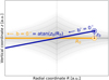 |
Fig. 1. Sketch illustrating the different line-of-sight integration paths for the same apparent latitude angle, b/b′, as determined by the vertical position of the Sun, z0, at fixed radial position, R0. |
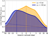 |
Fig. 2. Longitude-averaged line-of-sight integration of the same exponential disc (Re, he) = (3.5, 0.1) 3D emissivity model as a function of latitude for vertical positions of 0 (symmetric, orange) and +50 pc (violet). In the symmetric case, the emission peaks at b = 0°, as expected, and already for z0 = 50 pc, the peak is shifted 3° to negative latitudes. See text for further details and implications. |
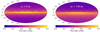 |
Fig. 3. Line-of-sight integrated emissivities of the same exponential disc (Re, he) = (3.5, 0.1) model as a function of longitude and latitude for z0 = 0 (left) and +50 pc (right). The images have been normalised to the symmetric case and thus contain the same absolute flux. Clearly, the contrast in the right image is higher, but the flux is more spread out into a larger number of pixels. |
These detailed peculiarities can be used to determine z0 from γ-ray emission alone. In the following Sect. 2.2, the basics about the spectrometer on board the International Gamma-Ray Astrophysics Laboratory (INTEGRAL/SPI), the chosen data set, and model fitting in its raw photon-count data space are explained.
2.2. Instrument, data, and fit
The spectrometer SPI (Vedrenne et al. 2003) on board ESA’s INTEGRAL satellite (Winkler et al. 2003) measures photons in the energy range between 20 and 8000 keV with a 19-element high-purity Ge detector camera. It uses a coded-mask technique to distinguish between emission from the sky and typically high instrumental background radiation from the telescope and satellite themselves. SPI has a field of view of 16° and an angular resolution of 2.7°. The data space is thus a size-19 vector of photon counts at different energies for individual pointed observations (“pointings”) of typically 30 min duration. Because we study one of the strongest γ-ray lines, we summed all counts between 1805 and 1813 keV into one 8 keV broad energy bin, corresponding to three times the spectral resolution of SPI at 1.8 MeV. In this study, we do not aim for optimising or characterising the 26Al emission morphology, nor are we interested in the detailed spectral shape of the emission line.
Our data set consists of 200 Ms of INTEGRAL/SPI observation time, distributed predominantly in the centre of the Galaxy as well as the Galactic plane, with a patchy exposure at higher latitudes2. In total, more than 13 years of data are accumulated, resulting in Nobs = 92 867 pointings of consecutive size-19 vectors. When the imaging response, Rjp, is applied for each pixel j ∈ (l, b)j in each pointing p ∈ Nobs, to the emission model Flos(l, b)j, this translates an image or model of the sky,  , into the SPI data space for a particular set of observations:
 (5)
(5)
In Eq. (5), the absolute flux normalisation, Fnorm, is determined through a maximum likelihood fit, and z0 is a free parameter (see below). Understanding the instrumental background in γ-ray astrophysics is key to any parameter inference. Details about robust and reliable background modelling with SPI can be found in Diehl et al. (2018b) and Siegert et al. (2019). Here, the background is modelled as a combination of contributions from the instrumental continuum,  , as well as instrumental lines,
  , and their absolute levels are determined through a (time-dependent) scaling parameter in a fit again. The total model thus writes
 (6)
(6)
In this full forward-modelling manner, the parameters Fnorm,  , and
, and  are straightforwardly determined by maximising the Poissonian likelihood function,
 (7)
(7)
because they are linear parameters. However, the convolution of Flos(l, b; z0)j with Rjp is computationally very expensive and would be required in each iteration of the fit to determine the unknown parameter z0 because it is changing the appearance of  . We therefore fixed it for a particular fit, and evaluated the likelihood for a pre-defined set of z0 values. Here, we used a grid of 15 vertical extents, ranging between −20 and +130 pc in steps of 10 pc. These values are based on a canonical distance of 8.5 kpc to the Galactic centre. Because the problem is geometrically similar, a correction factor R0/8.5 kpc = 0.9621 can be applied to each z0 value for a correct estimate given the more precise measurements of R0 by Abuter et al. (2019), or 0.9348 from the R0 estimate by Do et al. (2019).
3. Results
We used two examples to estimate the vertical position of the Sun from emission of the 26Al decay line. The emission in both cases is characterised by the doubly exponential disc model, Eq. (1), but with two assumptions on the radial and vertical scale parameters: Wang et al. (2009) suggested an exponential scale height at 1.8 MeV of  pc at a distance to the Galactic centre of 8.5 kpc. This estimate is based on a fixed scale radius of 3.5 kpc and only considers the sky region |l|< 60°, |b|< 30°. Siegert (2017) used the data set described in this work and performed exponential disc fits, including the full sky and varying both scale dimensions. This resulted in an estimate of Re = 5.6 ± 0.6 kpc and ze = 670 ± 190 pc for 26Al. We scaled and re-weighted the parameter sets of Wang et al. (2009) and Siegert (2017), resulting in the combinations (Re, ze) = (3.37, 0.15) and (4.81, 0.46), respectively. In a common reference system with R0 = 8.178 kpc, we finally performed the above-described maximum likelihood fits. These two examples serve as a proof-of-concept study that uses the two extreme values reported in the recent literature.
The probability density functions of z0, given the two models, are shown in Fig. 4. The more concentrated emission model with small-scale dimensions results in a vertical position of the Sun above the Galactic midplane of 7 ± 9 pc. The larger-scale dimensions, as suggested from the full-sky model fits, result in z0 = 15 ± 17 pc. These values are consistent with each other and also consistent with the median of 56 previous completely independent measurements using different techniques, giving ≈17 pc in a range between 5 and 29 pc (Karim & Mamajek 2017). While the model with a narrower emission morphology provides smaller uncertainties, it was shown that larger scale radii and heights are apparently needed to cover the entire3 Milky Way emission at 1.8 MeV (Siegert 2017). We therefore quote the larger uncertainty as a more conservative estimate. A more detailed model to describe the true 26Al morphology in the Galaxy might even now result in a much more accurate estimate of z0. The structural details of the 26Al emission in the Milky Way are beyond the scope of this paper because the goal is to show the feasibility of such a measurement with currently available data in the soft γ-ray regime
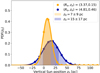 |
Fig. 4. Probability distribution functions for the vertical position of the Sun using INTEGRAL/SPI 26Al data and two different exponential disc models. In this range of plausible models, the position is constrained between in the interval [−2, 32] pc, consistent with independent estimates. |
4. Vertical emission extents and bias
This remarkable and unexpectedly good result leads to the question whether there might be biases in estimating the spatial extents of MeV γ-ray emission. In particular, setting the vertical position of the observer incorrectly in a typical analysis, for example, intending to measure the exponential scale height, may result in over- or underestimating the vertical extent of the emission.
We investigated this potential bias by fitting exponential disc models with z0 = 0 to simulations of models with z0 ≠ 0, and varying the scale height he. In this way, we determined an optimal scale height that differs from the input model if the correct position of z0 is not met. We chose three different sets of (Re, ze), (7.00, 0.30), (3.50, 0.10), and (5.00, 0.02), and performed a scan of he for each value of z0. The resulting relative deviations for our three test cases are shown in Fig. 5. If the vertical position z0 = 0 is met, the relative deviation from the correct scale height is by definition equal to zero. Because this problem is again symmetric, we only show positive values of z0. The larger the true scale height, the smaller the relative deviation from using an incorrect observer position. In the case of (Re, ze) = (7.00, 0.30), for example, the relative deviation inside the z0-position interval determined from γ-rays is up to 20%. This value is comparable to the uncertainty of the 26Al scale height determined by Siegert (2017) (< 30%) and should therefore be carefully considered when new or updated measurements in the MeV regime are discussed. In the case of smaller true scale heights, the effect of choosing an incorrect observer position is even more severe and ranges up to 50% (125%) when scale heights as small as 100 pc (20 pc) are considered.
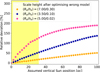 |
Fig. 5. Relative deviations, True − Fitted/True × 100%, of doubly exponential and change throughout for consistency disc models as a function of z0 and ze (ze = 300 pc orange, 100 pc violet, and 20 pc pink), fitted by a z0 = 0 model, assuming the correct Re. The yellow region determines the 1σ uncertainty from the z0 fit from 1.8 MeV data alone, see Sect. 3. By definition, the z0 = 0 case yields a relative deviation of zero. |
5. Conclusion
Using 13 years of 26Al data at 1.8 MeV from INTEGRAL/SPI, we determined the vertical position of the Sun above the Galactic midplane to z0 = 15 ± 17 pc in a proof-of-concept study. This is a remarkable result, both in terms of accuracy and precision: current soft γ-ray telescopes suffer from the “MeV gap” in sensivity (e.g. De Angelis et al. 2018; Timmes et al. 2019; Tomsick et al. 2019), which most of the time allows them to only study the sources inside, or the Milky Way itself. The statistical uncertainties on z0 we estimate from only using INTEGRAL/SPI data and a simple first-order analytic geometric model are only a factor of a few away from the most precise measurements using star counts or H II regions (17 ± 2 pc), which show a systematic spread of ≈12 pc (Karim & Mamajek 2017), however. A more detailed geometric model of 26Al would already provide similar uncertainties in z0 with current instrumentation. In consequence, the accuracy of this measurement can imply biases in determining other emission parameters, such as its vertical extent (latitudinal or exponential scale height). We find that specifically for 26Al, the relative uncertainty of scale heights as a function of z0 can be up to 25% (or higher for smaller scale heights than 26Al). This value is comparable to the uncertainties from scale-height measurements themselves, and may lead to misestimates (in both directions) of the true scale height. Consequently, z0 should be carefully considered in future modelling of the MeV γ-ray sky.
We note that Compton telescopes are barely affected by this circumstance because they locate the emission based on the more unique Compton scattering response. See e.g. the Compton Spectrometer and Imager, COSI (Kierans et al. 2016; Tomsick et al. 2019).
See http://www2011.mpe.mpg.de/gamma/instruments/integral/spi/www/public_data/index.html for a current exposure map.
Combinations of small and large scale heights provide an estimate of how much emission comes from the solar vicinity (Siegert 2017), but this is very degenerate in the SPI data space and was thus not considered here as a third case.
Acknowledgments
Thomas Siegert is supported by the German Research Society (DFG-Forschungsstipendium SI 2502/1-1).
References
- Abuter, R., Amorim, A., Bauboeck, M., et al. 2019, A&A, 625, L10 [NASA ADS] [CrossRef] [EDP Sciences] [Google Scholar]
- Allain, M., & Roques, J. P. 2006, A&A, 447, 1175 [NASA ADS] [CrossRef] [EDP Sciences] [Google Scholar]
- Blaauw, A., Gum, C. S., Pawsey, J. L., & Westerhout, G. 1960, MNRAS, 121, 123 [NASA ADS] [CrossRef] [Google Scholar]
- Bonatto, C., Kerber, L. O., Bica, E., & Santiago, B. X. 2006, A&A, 446, 121 [NASA ADS] [CrossRef] [EDP Sciences] [Google Scholar]
- Bouchet, L., Jourdain, E., & Roques, J. P. 2015, ApJ, 801, 142 [NASA ADS] [CrossRef] [Google Scholar]
- Buckner, A. S. M., & Froebrich, D. 2014, MNRAS, 444, 290 [NASA ADS] [CrossRef] [Google Scholar]
- De Angelis, A., Tatischeff, V., Grenier, I. A., et al. 2018, J. High Energy Astrophys., 19, 1 [NASA ADS] [CrossRef] [Google Scholar]
- Diehl, R., Halloin, H., Kretschmer, K., et al. 2006, Nature, 439, 45 [NASA ADS] [CrossRef] [PubMed] [Google Scholar]
- Diehl, R., Hartmann, D. H., & Prantzos, N. 2018a, in Astrophysics with Radioactive Isotopes (Springer, Cham), Astrophysics and Space Science Library, 453 [CrossRef] [Google Scholar]
- Diehl, R., Siegert, T., Greiner, J., et al. 2018b, A&A, 611, A12 [NASA ADS] [CrossRef] [EDP Sciences] [Google Scholar]
- Do, T., Hees, A., Ghez, A., et al. 2019, Science, 365, 664 [NASA ADS] [CrossRef] [Google Scholar]
- Elias, F., Cabrera-Caño, J., & Alfaro, E. J. 2006, AJ, 131, 2700 [NASA ADS] [CrossRef] [Google Scholar]
- Freudenreich, H. T. 1998, AJ, 492, 495 [NASA ADS] [CrossRef] [Google Scholar]
- Gum, C. S., Kerr, F. J., & Westerhout, G. 1960, MNRAS, 121, 132 [NASA ADS] [CrossRef] [Google Scholar]
- Joshi, Y. C., Dambis, A. K., Pandey, A. K., & Joshi, S. 2016, A&A, 593, A116 [NASA ADS] [CrossRef] [EDP Sciences] [Google Scholar]
- Jurić, M., Ivezić, Ž., Brooks, A., et al. 2008, AJ, 673, 864 [Google Scholar]
- Karim, M. T., & Mamajek, E. 2017, MNRAS, 465, 72 [Google Scholar]
- Kierans, C., Boggs, S., Chiu, J. L., et al. 2016, in Proc. 11th INTEGRAL Conf. Gamma-Ray Astrophysics in Multi-Wavelength Perspective, 10–14 October 2016 Amsterdam, 75 [Google Scholar]
- Knödlseder, J., Prantzos, N., Bennett, K., et al. 1996, A&AS, 120, 335 [NASA ADS] [Google Scholar]
- Knödlseder, J., Jean, P., Lonjou, V., et al. 2005, A&A, 441, 513 [NASA ADS] [CrossRef] [EDP Sciences] [Google Scholar]
- Krause, M., Diehl, R., Böhringer, H., Freyberg, M., & Lubos, D. 2014, A&A, 566, A94 [NASA ADS] [CrossRef] [EDP Sciences] [Google Scholar]
- Krause, M. G. H., Diehl, R., Bagetakos, Y., et al. 2015, A&A, 578, A113 [NASA ADS] [CrossRef] [EDP Sciences] [Google Scholar]
- Kretschmer, K., 2011, PhD Thesis, Technische Universität München, München [Google Scholar]
- Kretschmer, K., Diehl, R., Krause, M., et al. 2013, A&A, 559, A99 [NASA ADS] [CrossRef] [EDP Sciences] [Google Scholar]
- Majaess, D. J., Turner, D. G., & Lane, D. J. 2009, MNRAS, 398, 263 [NASA ADS] [CrossRef] [Google Scholar]
- Mendez, R. A., & van Altena, W. F. 1998, A&A, 330, 910 [NASA ADS] [Google Scholar]
- Oberlack, U., Bennett, K., Bloemen, H., et al. 1996, A&AS, 120, C311 [NASA ADS] [Google Scholar]
- Olausen, S. A., & Kaspi, V. M. 2014, ApJS, 212, 6 [NASA ADS] [CrossRef] [Google Scholar]
- Paladini, R., Burigana, C., Davies, R. D., et al. 2003, A&A, 397, 213 [NASA ADS] [CrossRef] [EDP Sciences] [Google Scholar]
- Peretto, N., & Fuller, G. A. 2009, A&A, 505, 405 [NASA ADS] [CrossRef] [EDP Sciences] [Google Scholar]
- Siegert, T. 2017, PhD Thesis, Technische Universität München, Published online at https://mediatum.ub.tum.de/node?id=1340342 [Google Scholar]
- Siegert, T., Diehl, R., Weinberger, C., et al. 2019, A&A, 626, A73 [NASA ADS] [CrossRef] [EDP Sciences] [Google Scholar]
- Simpson, R. J., Povich, M. S., Kendrew, S., et al. 2012, MNRAS, 424, 2442 [NASA ADS] [CrossRef] [Google Scholar]
- Skowron, D. M., Skowron, J., Mróz, P., et al. 2019, Science, 365, 478 [NASA ADS] [CrossRef] [Google Scholar]
- Timmes, F., Fryer, C., Hungerford, A. L., et al. 2019, Astrophys., 51, 2 [NASA ADS] [Google Scholar]
- Tomsick, J. A., Zoglauer, A., Sleator, C., et al. 2019, ArXiv e-print [arXiv:1908.04334] [Google Scholar]
- Vedrenne, G., Roques, J. P., Schönfelder, V., et al. 2003, A&A, 411, L63 [NASA ADS] [CrossRef] [EDP Sciences] [Google Scholar]
- Wang, W., Lang, M. G., Diehl, R., et al. 2009, A&A, 496, 713 [NASA ADS] [CrossRef] [EDP Sciences] [Google Scholar]
- Winkler, C., Courvoisier, T. J. L., Di Cocco, G., et al. 2003, A&A, 411, L1 [NASA ADS] [CrossRef] [EDP Sciences] [Google Scholar]
All Figures
|
Fig. 1. Sketch illustrating the different line-of-sight integration paths for the same apparent latitude angle, b/b′, as determined by the vertical position of the Sun, z0, at fixed radial position, R0. |
| In the text | |
|
Fig. 2. Longitude-averaged line-of-sight integration of the same exponential disc (Re, he) = (3.5, 0.1) 3D emissivity model as a function of latitude for vertical positions of 0 (symmetric, orange) and +50 pc (violet). In the symmetric case, the emission peaks at b = 0°, as expected, and already for z0 = 50 pc, the peak is shifted 3° to negative latitudes. See text for further details and implications. |
| In the text | |
|
Fig. 3. Line-of-sight integrated emissivities of the same exponential disc (Re, he) = (3.5, 0.1) model as a function of longitude and latitude for z0 = 0 (left) and +50 pc (right). The images have been normalised to the symmetric case and thus contain the same absolute flux. Clearly, the contrast in the right image is higher, but the flux is more spread out into a larger number of pixels. |
| In the text | |
|
Fig. 4. Probability distribution functions for the vertical position of the Sun using INTEGRAL/SPI 26Al data and two different exponential disc models. In this range of plausible models, the position is constrained between in the interval [−2, 32] pc, consistent with independent estimates. |
| In the text | |
|
Fig. 5. Relative deviations, True − Fitted/True × 100%, of doubly exponential and change throughout for consistency disc models as a function of z0 and ze (ze = 300 pc orange, 100 pc violet, and 20 pc pink), fitted by a z0 = 0 model, assuming the correct Re. The yellow region determines the 1σ uncertainty from the z0 fit from 1.8 MeV data alone, see Sect. 3. By definition, the z0 = 0 case yields a relative deviation of zero. |
| In the text | |
Current usage metrics show cumulative count of Article Views (full-text article views including HTML views, PDF and ePub downloads, according to the available data) and Abstracts Views on Vision4Press platform.
Data correspond to usage on the plateform after 2015. The current usage metrics is available 48-96 hours after online publication and is updated daily on week days.
Initial download of the metrics may take a while.