| Issue |
A&A
Volume 632, December 2019
|
|
|---|---|---|
| Article Number | A35 | |
| Number of page(s) | 7 | |
| Section | Astrophysical processes | |
| DOI | https://doi.org/10.1051/0004-6361/201936064 | |
| Published online | 25 November 2019 | |
Closing the gap to convergence of gravitoturbulence in local simulations⋆
1
Institut für Theoretische Physik und Astrophysik, Christian-Albrechts-Universität zu Kiel, Leibnizstr. 15, 24118 Kiel, Germany
e-mail: This email address is being protected from spambots. You need JavaScript enabled to view it.
2
Hamburger Sternwarte, Universität Hamburg, Gojenbergsweg 112, 21029 Hamburg, Germany
3
Steward Observatory, The University of Arizona, 933 N. Cherry Ave., Tucson, AZ 85721, USA
Received:
11
June
2019
Accepted:
19
September
2019
Abstract
Aims. Our goal is to find a converged cooling limit for fragmentation in self-gravitating disks. This is especially interesting for the formation of planets, brown dwarfs, or stars, and the growth of black holes. While investigating the limit, we want to give a clear criterion for the state of convergence.
Methods. We ran two-dimensional shearingsheet simulations with the hydrodynamic package Fosite at high resolutions. Thereby, resolution and limiters were altered. Subsequently, we investigated the spectra of important physical quantities at the length scales where fragmentation occurs. In order to avoid prompt fragmentation at high resolutions, we started these simulations with a fully-developed gravitoturbulent state obtained at a lower resolution.
Results. We show nearly converged results for fragmentation with a critical-cooling timescale tcrit ∼ 10 Ω−1. We can backtrace this claim by investigating the spectra of relevant physical variables at length scales around and below the pressure scale height. We argue that well-behaved results cannot be expected if counteracting quantities vary too much on these critical-length scales, either by change of resolution or numerical method. A comparison of fragmentation behaviour with the related spectra reveals that simulations behave similar, if the spectra are converged to the length scales where self-gravity leads to instabilities. Observable deviations in the results obtained with different numerical setups are confined to scales below these critical length scales.
Key words: instabilities / hydrodynamics / protoplanetary disks / accretion / accretion disks / methods: numerical
Two movies associated to Figs. 1 and 2 are available at https://www.aanda.org
© ESO 2019
1. Introduction
Self-gravitating disks play an import role in the field of young protoplanetary disks and active galactic nuclei (AGN). A disk becomes gravitationally unstable if the Toomre parameter
 (1)
(1)
fulfils Q < 1 (Toomre 1964). Thereby, κ is the epicyclic frequency, which becomes the angular velocity Ω in the case of a Keplerian disk, cs is the sound speed, G the gravitational constant, and Σ the surface density. The Toomre criterion is viable in a local approximation with axisymmetric potential.
Local gravitation acts on a certain length scale interval, where disturbances are allowed to grow (Toomre 1964; Lin & Pringle 1987). It is determined by the critical-length scale as an upper limit Lcrit = GΣ/Ω2, and by the Jeans length scale  as a lower limit. Thus, perturbances within
 (2)
(2)
are amplified, and could eventually lead to fragmentation. Nelson (2006) imposed numerical consequences for this, and stated that the Toomre-wavelength λT = 2LJ ∼ H needs to be resolved by a simulation, where H = cs/Ω is the Keplerian scale height.
Gammie (2001) showed numerically in his paper that a slow-cooling disk settles into the gravitoturbulent state (Paczynski 1978), whereas a gravitationally unstable disk that cools fast leads to fragmentation. In the former case, turbulence leads to an enhanced transport of angular momentum (Lin & Pringle 1987; Balbus & Papaloizou 1999; Duschl et al. 2000; Duschl & Britsch 2006). In the latter, the gaseous disk may at least partly disintegrate if giant planets, brown dwarfs or, in case of AGN disks, even massive stars, form within the disk (Rice et al. 2015; Baehr et al. 2017; Boss 1998; Levin & Beloborodov 2003). The criterion for fragmentation that Gammie (2001) ascertains is that the cooling fulfils β = tcΩ < 3, where β is a dimensionless quantity describing the cooling timescale tc in terms of orbital timescale Ω−1. The value for β can also be related to an effective viscosity parameter α = (γ(γ−1)q2β)−1 (Gammie 2001; Shakura & Sunyaev 1973). Here, γ is the ratio of specific heat capacities, and  is the power-law exponent of the rotation law, which becomes 3/2 for Keplerian motion.
However, simulations also show fragmentation for larger β, while going to higher resolutions (Meru & Bate 2011; Paardekooper et al. 2011). This non-convergence also takes place in the local-approximation (Paardekooper 2012; Baehr & Klahr 2015; Klee et al. 2017). Even by using altered cooling on small scales, Baehr & Klahr (2015) suffer from fragmentation in their high-resolution runs. Recently, Deng et al. (2017) showed that codes that rely on smoothed-particle hydrodynamics that use artificial viscosity also have problems with artificial fragmentation. This can be circumvented by using meshless methods. But also, grid-based codes with shock capturing mechanisms can get into trouble, where limiting functions can have a strong impact on the outcome of the simulations Klee et al. (2017).
Young & Clarke (2015) also observed fragmentation above the critical βcrit in their simulations. They proposed that a quasi-static collapse can explain this behaviour. Paardekooper (2012) shows that there is also a stochastic component when running over long timescales.
More recently, three dimensional shearingbox simulations were also carried out in the local approximation (Shi & Chiang 2014). Baehr et al. (2017) found fragmentation at around β ≲ 3 reaching high resolutions with very small box-sizes. Riols et al. (2017) show that, at sufficiently high resolutions, small-scale turbulences set in, off the midplane. They furthermore point out that the energy spectrum of gravitoturbulence can be approximated by the k−5/3 cascade (Kolmogorov 1941). However, they raise the problem already revealed by Gammie (2001) that in order to have a well-behaved gravitoturbulent state, the box size should be not too small. They conclude the necessity for a box size of at least ≳40 H = 40πLcrit. Otherwise, bursts that might be connected to transient fragmentation set in. Booth & Clarke (2018) propose a minimal size of the shearingbox ≳64 H in the horizontal direction. Otherwise, long-term trends show up.
In this paper, we investigate fragmentation at very high horizontal resolutions while preserving a well-behaved gravitoturbulent state in a sufficiently large shearing sheet. We first describe our methods in Sect. 2, explaining the underlying equations and the setup. In Sect. 3, we present the numerical results obtained for highest resolutions and close to converged spectra for various quantities. Finally, we discuss and conclude our results in Sect. 4.
2. Methods
We used the hydrodynamic code Fosite by Illenseer & Duschl (2009), a generalised version of the finite volume method of Kurganov & Tadmor (2000). Fosite can operate on arbitrary curvilinear-orthogonal grids and is fully parallelised and vectorised. It uses modern Fortran 2008 language features and object-oriented design patterns. Fosite has recently been ported and optimised for the new NEC SX-Aurora Tsubasa vector computer, which gave us the ability to carry out simulations with unprecedented high-resolution in two dimensions1.
2.1. Hydrodynamic equations
We solved the two-dimensional hydrodynamical equations in the local approximation (Goldreich & Lynden-Bell 1965; Hawley et al. 1995). Together with the Poisson equation for a razor thin disk (Gammie 2001), the system of equations is,
 (3)
(3)
 (4)
(4)
 (5)
(5)
 (6)
(6)
Here, p is the integrated pressure, and  is the residual part of the two-dimensional velocity, by the splitting of a background velocity
  . The according total energy is
  . The additional advection step, which is the last term on the left hand side of Eqs. (3)–(5), is calculated separately in order to allow for very large time steps (Masset 2000; Jung et al. 2018). The gravitational potential of the shearingsheet Φsg describes the self-gravitation. Thereby, δ(z) is the delta-distribution. The according Poisson Eq. (6) is solved in Fourier space (Gammie 2001; Klee et al. 2017), imposing periodic boundary conditions. This is achieved by shifting the whole density field to the next periodic point before applying the transformation (Gammie 2001; Klee et al. 2017). Finally,
  is the well-known cooling parametrisation (Gammie 2001).
2.2. Numerical setup
In order to have a well-tuned setup, we relied on the results in Klee et al. (2017). There, different numerical shock-capturing mechanisms (limiting functions) were tested against each other. We thus prefer van-Leer limiting (van Leer 1974), which proved to be advantageous in contrast to other limiting functions, regarding artificial fragmentation. However, most simulations were again carried out using the Superbee limiter (Roe & Baines 1982) for comparison. Additionally, we used Dormand-Prince time stepping (Dormand & Prince 1980), which showed the best results in the epicyclic motion test (Klee et al. 2017).
We rotated the computational domain by 90° in contrast to Klee et al. (2017). This was advantageous as it made the first dimension completely accessible for the parallel Fourier solver, while preserving vectorisation. We thus decomposed the grid in pencils along the y-direction.
2.3. Simulation setup
With Lx = Ly = 320 Lcrit, we used the same grid size as in Gammie (2001). This corresponds to ∼100 H. It ensured that we were not getting into trouble with long-term periodics as stated in Booth & Clarke (2018). Another reason for staying with a relatively large extent of the box compared to other three-dimensional simulations is already given by Gammie (2001, Fig. 9). There, the contribution of the gravitational component of the stress is taken into consideration for twice our size L = 640 Lcrit. Taking the length of L = 320 Lcrit into account, this still includes ∼90% of the gravitational component. Further reduction of box size removed a significant amount of gravitational stress from the simulations that may have had a major impact on the results. This is supported by the observations of Riols et al. (2017) and Booth & Clarke (2018), who found that while some parameters, like Toomre’s Q converge quite quickly for increasing box sizes, kinetic energy and gravitational stress do not.
We used γ = 2.0 in order to conform to previous results (Gammie 2001; Paardekooper 2012; Klee et al. 2017). It should be kept in mind, however, that smaller γ generally increase the probability of fragmentation (Rice 2016).
Booth & Clarke (2018) investigated in more detail the problem of prompt fragmentation, where fragments form during initialisation. In Klee et al. (2017), we already used the approach of slowly moving down the cooling in order to prevent this kind of fragmentation in local simulations. However, going to higher resolutions made it increasingly harder for us to prevent the artificial fragmentation in this manner. Additionally, reaching the gravitoturbulent state needs more and more time for higher resolutions and slower (initial) cooling.
In this work, we take another approach. Instead of fine-tuning the initial cooling, we reuse the result of a previous fully-developed low-resolution run with slow cooling using spline-interpolation to generate high resolution data2. Thereby, we already initiate the high-resolution simulation with a gravitoturbulent state. This approach also saves a significant amount of computational time skipping the initial phase in which the simulation settles into the gravitoturbulent state.
3. Simulations and results
Table 1 shows an overview of the simulations that were done. We ran simulations at twice and four times the highest resolution in Klee et al. (2017), which corresponds to a resolution of 4096 and 8192, respectively.
Overview of simulation runs.
As initial conditions for the runs with resolution 4096, we used a gravitoturbulent run with a resolution of 2048, van-Leer limiting, and β = 10. Since our run at β = 10 fragmented at a resolution of 4096, we used the run with β = 15 as a starting point for the runs with a resolution of 8192. At a resolution of 4096, the normal runtime is 200 Ω−1, and at 8192 it is 100 Ω−1. If many clear fragments formed, we stopped the run earlier. For small-density enhancements at the end of the run, we optionally extended the run to investigate its outcome.
In case of simulations carried out with the Superbee limiter, a close inspection of the region within y = ±20 Lcrit reveals small, almost circular features with unusual density depletions, which were never observed in simulations with the van-Leer limiter. It is not clear to us what determines the spatial occurrence and extent, as well as the lifetime of these structures. As a matter of fact, they seem to be continuously generated only around the midplane with scales of a few Lcrit at most, and are therefore only visible in the simulations at resolutions 4096 and 8192. If they encounter strong shocks, they are often completely destroyed, but some of them survive for several orbital time scales.
We think that these structures are numerical artefacts, again caused by oversteepening (Klee et al. 2017). Since the Superbee limiter tends to overestimate spatial gradients, it amplifies low-pressure areas. The results shown for the isentropic vortex test Yee et al. (1999) in Appendix A support this hypothesis. They clearly illustrate that the Superbee limiter enhances the central pressure trough, while the van-Leer limiter depletes it.
Figures 1–3 show snapshots of the high-resolution results obtained with different limiters and cooling parameters. In case of the gravitoturbulent simulations, we also provide movies for better illustration of what is going on in these simulations, and to make the differences between the two limiters clearer.
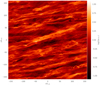 |
Fig. 1. Snapshot of surface density of gravitoturbulent state at a resolution of 8192 for β = 10 and van-Leer limiting. This simulation shows later fragments with 20 − 30 times the background density. |
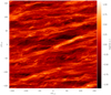 |
Fig. 2. Snapshot of surface density of gravitoturbulent state at a resolution of 8192 for β = 10 and Superbee limiting. |
 |
Fig. 3. Snapshot of surface density in a fully fragmented run at a resolution of 8192 for β = 5 and van-Leer limiting. |
3.1. Fragmentation
Figure 4 summarises which simulations showed fragmentation. Besides the new runs, we also added the results for lower resolutions from Klee et al. (2017). For higher resolutions, the question of whether or not fragmentation occurs is less affected by the limiter. This is not what we would expect in view of our argumentation in Klee et al. (2017), where Superbee suffered from numerical errors that forced fragmentation. Looking at even higher resolutions, we see that the Superbee limiter does not fragment for β = 10. Thus, in contrast to our previous findings, it seems that the Superbee limiter yields similar results with respect to the fragmenting behaviour, and the threshold for fragmentation stabilises at around β ∼ 10.
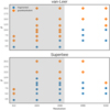 |
Fig. 4. Fragmentation plot for different resolutions N and cooling timescales β. The grey regions show results already published in Klee et al. (2017). The simulations seem to converge at the highest resolutions to a value of βcrit ≈ 10 for both numerical schemes. |
For β = 10 and van-Leer limiting at N = 4096, we had a single fragment that formed between 50 Ω−1 and 75 Ω−1, and it was disrupted again before the end of the run. On the other side, we had a fragment for the same setup with Superbee at the regular end of the simulation. We then extended the simulation another 50 Ω−1 in order to ensure that it would be stable for a longer period. A similar behaviour was found in the run with N = 8192 for van-Leer limiting and β = 10. In this case, a fragment forms around ∼80 Ω−1, which has 20 − 30 times the background density, and is stable for at least ∼40 Ω−1. Thus, only single or few fragments form in the range 5 < β ≲ 10, whereas below β = 5, the whole field fragments immediately (cf. Fig. 3). In addition, if β ∼ 10 these single fragments sometimes do not survive for longer periods. Therefore, the conclusion as to whether or not the simulation is fragmented seems less clear in these cases, since it depends on the formation and stability of a single fragment.
3.2. Convergence of spectra at important length scales
In Figs. 5 and 6, we show density and pressure spectra, respectively. The spectra are adopted for a cooling parameter of β = 10 at a state where fragmentation did not occur yet (if present). Thereby, their components in kx, ky, and k are displayed. We see most clearly in the surface density that the results obtained with low resolutions deviate significantly from those at higher resolutions, even on length scales of the order of the scale height and above. The plots show that runs at the same resolution, but with different limiters, can lead to a deviation in the spectra that is partially larger than an order of magnitude. Here, the difference between resolutions is of several magnitudes. At higher resolutions, we see that the spectral quantities are very similar and follow the cascade down to the scale height H. For many quantities, this is even true for the smaller length scale Lcrit, especially at the resolution of 8192. The x-components, which correspond in our case to the direction that is more parallel to the shock fronts, lacks a bit of convergence at least at the length scale Lcrit.
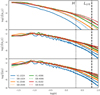 |
Fig. 5. Components of density spectrum for different resolutions and limiters. The density spectrum is well converged at highest resolutions to a length scale of H. The component in x-direction is only close to convergence down to Lcrit. |
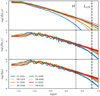 |
Fig. 6. Components of pressure spectrum for different resolutions and limiters. The pressure spectrum is well converged at highest resolutions even to a length scale of Lcrit. |
In Fig. 7, we show spectra of the kinetic energy. In contrast to Figs. 5 and 6, we do not show the components along kx or ky, but the kinetic energy associated with vx, vy, and |v|, always summed up along the radius in Fourier space k. We see in Fig. 7 that the ∝k−5/3-law is fairly good, which is to be expected in two dimensions at large scales (Kraichnan 1967).
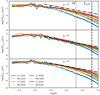 |
Fig. 7. Spectrum of kinetic energy for different resolutions and limiters. The velocities are summed up in Fourier space along the radius k. The spectrum fulfils the k−5/3 well at highest resolution down to Lcrit. |
All figures mentioned above show well-converged spectra at the scale height H at high resolutions. Additionally, they even have few differences at Lcrit. Having a look again at Fig. 4, we can state that the simulations that show differences with respect to fragmenting behaviour also show differences for the physical quantities at the length scales where fragmentation occurs. When this gap is closed, we also see smaller differences in the fragmenting behaviour. We thus have a clear criterion for convergence, which does not only rely on the observation of forming clumps, but on the turbulent cascade down to the relevant length scales.
4. Discussion and conclusion
We show results of self-gravitating shearing sheet simulations conducted in two dimensions at the highest resolution so far and investigate the fragmentation behaviour. In order to overcome prompt fragmentation, we interpolated from an already evolved gravitoturbulent state with lower resolutions, and used this as our initial conditions. However, even then we get a relatively large critical value of βcrit ≲ 10 as a fragmentation criterion. We regard this result as robust and independent of resolution as long as it exceeds 4096 at the least (40 cells per scale-height H). Still, there seems to be some uncertainty around the aforementioned βcrit swiftly declining for higher values. This holds also for different numerical schemes within the code, where we know that one of the limiting functions is prone to numerical errors. However, even with these errors, the critical value βcrit is not affected too much.
That is why we think that we are close to convergence. As a definition for that state we do not only have a look at the fragmentation behaviour with ever higher resolutions. Instead we investigate physical quantities of interest at the length scales where fragmentation occurs. When resolutions are high enough, the small scale structures show very clear cascades down to the length scales of interest in Eq. (2). Although even smaller structures can vary fundamentally between the numerical schemes, we get similar results for fragmentation. We conclude that the differences in the smallest structures have (nearly) no influence on the fragmentation process. This is the case, because the amplified modes by self-gravity only affect the length scales in Eq. (2).
Recent results prefer a clearer criterion at around βcrit = 3 (Baehr et al. 2017; Booth & Clarke 2018; Deng et al. 2017). They all have the advantage that they were run in three dimensions. However, in order to reach the necessary high horizontal resolutions, Baehr et al. (2017) and Booth & Clarke (2018) reduced the spatial dimensions (12 H and max. 32 H) for the runs in which they investigated fragmentation. Indeed we see that the runs where Booth & Clarke (2018) resolved H by 32 grid cells, show fragmentation for slightly larger βcrit ∼ 4. Interestingly, this corresponds to our runs between resolutions of 2048 and 4096 (cf. Fig. 4). Deng et al. (2017) also show that they see no fragmentation at higher resolutions with the meshless method code Gizmo (Hopkins 2014). They state this is due to the lack of artificial viscosity in these schemes. However, their code introduces slope limiting procedures, similar to those used in our code, Fosite, which evidentially impact the outcome of fragmentation studies (Klee et al. 2017).
It should also be taken into account that two-dimensional turbulence can behave differently when compared to three-dimensional turbulence. It has an additional turbulent energy cascade at small scales with ∝k−3 (Kraichnan 1967; Boffetta & Ecke 2012; Kolmogorov 1941). We see a fairly clear k−5/3 cascade down to Lcrit (cf. Fig. 7). On scales below Lcrit, however, the flow is no longer turbulent, because gravitational instabilities are not amplified anymore. Nevertheless, it would be interesting to carry out a similar analysis of converged spectra in three-dimensional simulations and verify these considerations.
The larger value of βcrit has some implications for fragmenting disks. Relating the critical cooling parameter to the effective viscosity parameter α yields a smaller critical value for this number, around αcrit ∼ 0.02 Gammie (2001). This would indeed mean that α-parametrisations with larger values might not be well-suited in the case of self-gravitating disks.
This reasoning becomes less clear if one takes additional heat sources into account. For example, Rice et al. (2011) show that an additional background irradiation cannot suppress fragmentation, but leads to fragmentation at smaller βcrit with smaller values for αcrit. The former direct relation between the two parameters is then disconnected. Even when the cooling is fast, the reachable value for αcrit becomes smaller.
In the case of protoplanetary disks, the shift to a larger value of a few for βcrit does not necessarily have a strong impact on the radial distance for fragmentation in a global setup. Generally, for larger βcrit, fragmentation can occur closer to the central object with a relation of β ∝ r−9/2 (Clarke & Lodato 2009). The cooling parameter thus strongly depends on the radius (Paardekooper 2012), which leads to little effect on radial change. The distance of formation would then still be at a radius of some ten astronomical units (Meru & Bate 2012). Regarding the lifetime of self-gravitating protoplanetary disks of ∼105 yr, (Laughlin & Bodenheimer 1994; Haisch et al. 2001) the results are still relevant. Taking into consideration a radius of r = 100 au, the disk would survive for ∼100 orbits, whereas the simulations of this work were done for up to 200 Ω−1, which would account for ∼32 orbits.
Finally, we come to the conclusion that while going to ever higher resolutions, we inevitably see again a shift to a larger βcrit ∼ 10, with some uncertainty around that value. While for β ≲ 5, the whole field fragments, and we see only single or a few fragments around 5 < β ≲ 10. Because of the close to converged spectra with different numerical setups, we do not expect this upper limit to change too much anymore.
Movies
Movie of Fig. 1 Access Supplementary Material
Movie of Fig. 2 Access Supplementary Material
The code is freely available under https://github.com/tillense/fosite
RegularGridInterpolator of the SciPy package (Jones et al. 2001).
Acknowledgments
We thank the anonymous referee for the very helpful comments and suggestions on a more recent version of this publication.
References
- Baehr, H., & Klahr, H. 2015, ApJ, 814, 155 [Google Scholar]
- Baehr, H., Klahr, H., & Kratter, K. M. 2017, ApJ, 848, 40 [NASA ADS] [CrossRef] [Google Scholar]
- Balbus, S. A., & Papaloizou, J. C. 1999, ApJ, 521, 650 [NASA ADS] [CrossRef] [Google Scholar]
- Boffetta, G., & Ecke, R. E. 2012, Ann. Rev. Fluid Mech., 44, 427 [NASA ADS] [CrossRef] [Google Scholar]
- Booth, R. A., & Clarke, C. J. 2018, MNRAS, 483, 3718 [NASA ADS] [CrossRef] [Google Scholar]
- Boss, A. P. 1998, ApJ, 503, 923 [NASA ADS] [CrossRef] [Google Scholar]
- Clarke, C., & Lodato, G. 2009, MNRAS, 398, L6 [NASA ADS] [CrossRef] [Google Scholar]
- Deng, H., Mayer, L., & Meru, F. 2017, ApJ, 847, 43 [NASA ADS] [CrossRef] [Google Scholar]
- Dormand, J. R., & Prince, P. J. 1980, J. Comput. Appl. Math., 6, 19 [CrossRef] [MathSciNet] [Google Scholar]
- Duschl, W. J., & Britsch, M. 2006, ApJ, 653, L89 [NASA ADS] [CrossRef] [Google Scholar]
- Duschl, W. J., Strittmatter, P. A., & Biermann, P. L. 2000, A&A, 357, 1123 [NASA ADS] [Google Scholar]
- Gammie, C. F. 2001, ApJ, 553, 174 [NASA ADS] [CrossRef] [Google Scholar]
- Goldreich, P., & Lynden-Bell, D. 1965, MNRAS, 130, 125 [NASA ADS] [CrossRef] [Google Scholar]
- Haisch, Jr., K. E., Lada, E. A., & Lada, C. J. 2001, ApJ, 553, L153 [NASA ADS] [CrossRef] [Google Scholar]
- Hawley, J. F., Gammie, C. F., & Balbus, S. A. 1995, ApJ, 440, 742 [NASA ADS] [CrossRef] [Google Scholar]
- Hopkins, P. F. 2014, Astrophysics Source Code Library [record ascl:1410.003] [Google Scholar]
- Illenseer, T. F., & Duschl, W. J. 2009, Comput. Phys. Commun., 180, 2283 [NASA ADS] [CrossRef] [Google Scholar]
- Jones, E., Oliphant, T., Peterson, P., et al. 2001, SciPy: Open Source Scientific Tools for Python [Online; accessed February 20, 2019] [Google Scholar]
- Jung, M., Illenseer, T. F., & Duschl, W. J. 2018, ArXiv e-prints [arXiv:1803.02055] [Google Scholar]
- Klee, J., Illenseer, T. F., Jung, M., & Duschl, W. J. 2017, A&A, 606, A70 [NASA ADS] [CrossRef] [EDP Sciences] [Google Scholar]
- Kolmogorov, A. N. 1941, Cr Acad. Sci. URSS, 30, 301 [Google Scholar]
- Kraichnan, R. H. 1967, Phys. Fluids, 10, 1417 [NASA ADS] [CrossRef] [Google Scholar]
- Kurganov, A., & Tadmor, E. 2000, J. Comput. Phys., 160, 241 [Google Scholar]
- Laughlin, G., & Bodenheimer, P. 1994, ApJ, 436, 335 [NASA ADS] [CrossRef] [Google Scholar]
- Levin, Y., & Beloborodov, A. M. 2003, ApJ, 590, L33 [NASA ADS] [CrossRef] [Google Scholar]
- Lin, D., & Pringle, J. 1987, MNRAS, 225, 607 [NASA ADS] [CrossRef] [Google Scholar]
- Masset, F. 2000, A&AS, 141, 165 [NASA ADS] [CrossRef] [EDP Sciences] [Google Scholar]
- Meru, F., & Bate, M. R. 2011, MNRAS, 411, L1 [NASA ADS] [CrossRef] [Google Scholar]
- Meru, F., & Bate, M. R. 2012, MNRAS, 427, 2022 [NASA ADS] [CrossRef] [Google Scholar]
- Nelson, A. F. 2006, MNRAS, 373, 1039 [NASA ADS] [CrossRef] [Google Scholar]
- Paardekooper, S.-J. 2012, MNRAS, 421, 3286 [NASA ADS] [CrossRef] [Google Scholar]
- Paardekooper, S.-J., Baruteau, C., & Meru, F. 2011, MNRAS, 416, L65 [NASA ADS] [CrossRef] [Google Scholar]
- Paczynski, B. 1978, Acta Astron., 28, 91 [Google Scholar]
- Rice, K. 2016, PASA, 33, e053 [NASA ADS] [CrossRef] [Google Scholar]
- Rice, W., Armitage, P., Mamatsashvili, G., Lodato, G., & Clarke, C. 2011, MNRAS, 418, 1356 [NASA ADS] [CrossRef] [Google Scholar]
- Rice, K., Lopez, E., Forgan, D., & Biller, B. 2015, MNRAS, 454, 1940 [NASA ADS] [CrossRef] [Google Scholar]
- Riols, A., Latter, H., & Paardekooper, S.-J. 2017, MNRAS, 471, 317 [NASA ADS] [CrossRef] [Google Scholar]
- Roe, P. L., & Baines, M. 1982, J., 281 [Google Scholar]
- Shakura, N. I., & Sunyaev, R. A. 1973, A&A, 24, 337 [NASA ADS] [Google Scholar]
- Shi, J.-M., & Chiang, E. 2014, ApJ, 789, 34 [NASA ADS] [CrossRef] [Google Scholar]
- Toomre, A. 1964, ApJ, 139, 1217 [Google Scholar]
- van Leer, B. 1974, J. Comput. Phys., 14, 361 [NASA ADS] [CrossRef] [Google Scholar]
- Yee, H. C., Sandham, N. D., & Djomehri, M. J. 1999, J. Comput. Phys., 150, 199 [NASA ADS] [CrossRef] [MathSciNet] [Google Scholar]
- Young, M. D., & Clarke, C. J. 2015, MNRAS, 451, 3987 [NASA ADS] [CrossRef] [Google Scholar]
Appendix A: Vortex test cuts
In Fig. A.1, cuts of isentropic vortex tests are presented. The setup is described in Yee et al. (1999), and Jung et al. (2018). It has initial conditions
 (A.1)
(A.1)
 (A.2)
(A.2)
 (A.3)
(A.3)
 (A.4)
(A.4)
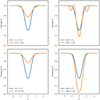 |
Fig. A.1. Cuts along x-axis at y = 0.0 for an isentropic vortex on a cartesian grid. Left (van-Leer): density and pressure are smeared out. Right (Superbee): density and pressure are both oversteepened with time. |
with density 𝜚, pressure p and vx, vy velocities in the according directions. The distance from the centre of the vortex is  . The other setup parameters are summarised in Table A.1.
Setup for isentropic vortex
The results with van-Leer and Superbee limiting show a qualitative difference regarding the evolution. With van-Leer, the vortex is smeared out, while with Superbee, the vortex is strengthened.
All Tables
All Figures
|
Fig. 1. Snapshot of surface density of gravitoturbulent state at a resolution of 8192 for β = 10 and van-Leer limiting. This simulation shows later fragments with 20 − 30 times the background density. |
| In the text | |
|
Fig. 2. Snapshot of surface density of gravitoturbulent state at a resolution of 8192 for β = 10 and Superbee limiting. |
| In the text | |
|
Fig. 3. Snapshot of surface density in a fully fragmented run at a resolution of 8192 for β = 5 and van-Leer limiting. |
| In the text | |
|
Fig. 4. Fragmentation plot for different resolutions N and cooling timescales β. The grey regions show results already published in Klee et al. (2017). The simulations seem to converge at the highest resolutions to a value of βcrit ≈ 10 for both numerical schemes. |
| In the text | |
|
Fig. 5. Components of density spectrum for different resolutions and limiters. The density spectrum is well converged at highest resolutions to a length scale of H. The component in x-direction is only close to convergence down to Lcrit. |
| In the text | |
|
Fig. 6. Components of pressure spectrum for different resolutions and limiters. The pressure spectrum is well converged at highest resolutions even to a length scale of Lcrit. |
| In the text | |
|
Fig. 7. Spectrum of kinetic energy for different resolutions and limiters. The velocities are summed up in Fourier space along the radius k. The spectrum fulfils the k−5/3 well at highest resolution down to Lcrit. |
| In the text | |
|
Fig. A.1. Cuts along x-axis at y = 0.0 for an isentropic vortex on a cartesian grid. Left (van-Leer): density and pressure are smeared out. Right (Superbee): density and pressure are both oversteepened with time. |
| In the text | |
Current usage metrics show cumulative count of Article Views (full-text article views including HTML views, PDF and ePub downloads, according to the available data) and Abstracts Views on Vision4Press platform.
Data correspond to usage on the plateform after 2015. The current usage metrics is available 48-96 hours after online publication and is updated daily on week days.
Initial download of the metrics may take a while.