| Issue |
A&A
Volume 632, December 2019
|
|
|---|---|---|
| Article Number | A41 | |
| Number of page(s) | 6 | |
| Section | Extragalactic astronomy | |
| DOI | https://doi.org/10.1051/0004-6361/201935620 | |
| Published online | 26 November 2019 | |
Quasar main sequence: A line or a plane
1
Center for Theoretical Physics, Polish Academy of Sciences, Al. Lotników 32/46, 02-668 Warsaw, Poland
e-mail: This email address is being protected from spambots. You need JavaScript enabled to view it.
, This email address is being protected from spambots. You need JavaScript enabled to view it.
2
Copernicus Astronomical Center, Bartycka 18, 00-716 Warsaw, Poland
Received:
4
April
2019
Accepted:
25
September
2019
Abstract
Context. A quasar main sequence is widely believed to reveal itself through objects represented in a plane spanned by two parameters: the full width at half maximum (FWHM) of Hβ and the ratio of Fe II to Hβ equivalent width. This sequence is related to the application to quasar properties of principal component analysis (PCA), which reveals that the main axis of variance (eigenvector 1) is codirectional with a strong anticorrelation between these two measurements.
Aims. We aim to determine whether the dominance of two eigenvectors, originally discovered over two decades ago, is replicated in newer high-quality quasar samples. If so, we aim to test whether a nonlinear approach is an improvement on the linear PCA method by finding two new parameters that represent a more accurate projection of the variances than the eigenvectors recovered from PCA.
Methods. We selected quasars from the X-shooter archive and a major quasar catalog to build high-quality samples. These samples were tested with PCA.
Results. We find that the new high-quality samples indeed have two dominant eigenvectors as originally discovered. Subsequently, we find that fitting a nonlinear decay curve to the main sequence allows a new plane spanned by linearly independent axes to be defined; this is based on the distance along the decay curve as the main axis and the distance of each quasar data point from the curve as the secondary axis, respectively.
Conclusions. The results show that it is possible to define a new plane based on the quasar main sequence, which accounts for the majority of the variance. The most likely candidate for the new main axis is an anticorrelation with a black hole mass. In this case the secondary axis likely represents luminosity. However, given the results of previous studies, the inclination angle likely plays a role in the Hβ width.
Key words: galaxies: active / quasars: general / accretion / accretion disks
© ESO 2019
1. Introduction
Active galactic nuclei (AGNs) are complex objects. They contain a central black hole that accretes surrounding material; the inflowing matter has large angular momentum and forms an accretion disk. This disk is the dominant radiating component in the brightest active nuclei, which are known as quasars (Peterson 1997). Although the accretion and radiation processes are complex, if we try to simplify the picture as much as possible we can reduce the number of parameters describing the active nucleus down to four: black hole mass, black hole spin, accretion rate (or, equivalently, the Eddington ratio), and viewing angle. In addition, we observe outflow phenomena (jets, winds), which are not necessarily uniquely determined by the parameters listed above and which considerably affect the observational properties of AGNs. Also, AGNs do not have to be well represented by a constant phenomenological type since changing-look AGNs (Matt et al. 2003) have recently been catching a lot of attention. If such changing-look events are not just related to temporary obscuration, the picture may be much more complicated.
Nevertheless, attempts have been made to simplify the picture through a determination of the most important parameters. In their pioneering paper in this field, Boroson & Green (1992) introduced principal component analysis PCA) as a method for understanding AGNs and showed that 13 measured quantities (e.g., line properties, multiband indices, and luminosity) can be combined into a sequence of eigenvectors of decreasing importance. The two most important eigenvectors were able to explain 51% of the variance in these properties, which were obtained from a sample of 87 objects. Their principal eigenvector (EV1) showed a strong anticorrelation between optical Fe II equivalent width (EW) and both optical [O III] EW and Hβ full width at half maximum (FWHM). This research was continued later (Sulentic et al. 2000, 2007; Marziani et al. 2001; Kuraszkiewicz et al. 2009) and led to the appearance of the term quasar main sequence, that is, analogous to the well-established stellar main sequence. This analysis works only for brighter AGN-like narrow line Seyfert 1 galaxies and quasars, and leaves out low-luminosity AGNs and blazars. Nevertheless it is an interesting step toward the identification of a few key properties.
Following on from these papers, the study by Shen & Ho (2014) claimed to have found a unified explanation for the EV1 behavior based on two parameters, namely the Eddington ratio and the quasar orientation. The plane of quasars on the FWHM(Hβ)–RFe II plane, where RFe II is the ratio of the EW of Fe II to the EW of Hβ, together with [O III] EW, is illustrated in their Fig. 1, showing the EV1 trends. It was theorized that increasing the Eddington ratio drives both an increasing RFe II and decreasing [O III] EW. The behavior of the Hβ FWHM was explained as a combination of black hole mass and orientation angle influences. However, this explanation is far from certain. For example, the measurement of Fe II strength is subject to uncertainties because of the broadened and heavily blended nature of the emission. Also, subsequent papers have called into question the accuracy of the RFe II measurements (Śniegowska et al. 2018) or have claimed the [O III] EW to be subject to the influence of orientation (Risaliti et al. 2011; Bisogni et al. 2017).
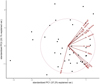 |
Fig. 1. Graphical representation of the PCA decomposition of the Capellupo sample reduced to 13 parameters. The dots represent individual objects on the standardized EV1–EV2 plane that have values indicated by the axis labels. The arrows represent the loadings of the variables in the EV1–EV2 plane; the unit circle is included for scale reference. |
In this paper we apply the PCA technique to two high-quality quasar samples using a different set of measured parameters than in previous studies. The aim is to check whether the minimum numbers of parameters (eigenvectors) needed to explain the majority of variance in the sample is a universal property of AGNs, and thus can indeed be used to identify the minimum number of key parameters needed to describe an active nucleus in a typical Seyfert 1 galaxy or quasar.
2. Using PCA for the analysis of quasar samples
A PCA analysis works by initially finding the principal axis along which the variance in the multidimensional space (corresponding to all recorded quasar properties) is maximized. This is known as eigenvector 1. Subsequent orthogonal eigenvectors, in order of decreasing variance along their respective directions, are found, until the entire parameter space is spanned. We analyzed two different quasar samples using the PCA method with the aim of determining the relative importance of the eigenvectors, and we supplement these with the previous results obtained for the PG quasar sample by Boroson & Green (1992). The key global parameters for these samples are given in Table 1.
Redshift and luminosity ranges of each sample.
2.1. PCA analysis of an X-shooter quasar sample
A high-quality sample of 30 quasar spectra, all located at similar redshifts (z ∼ 1.5), was collected and analyzed in a series of three papers dedicated to understanding quasar spectral energy distributions and accretion disks (Capellupo et al. 2015, 2016; Mejía-Restrepo et al. 2016); we hereafter refer to this as the Capellupo sample. These spectra were obtained using the X-shooter instrument on the Very Large Telescope (VLT), allowing observation of several important rest-frame ultraviolet (UV) and optical lines at the selected redshift. These sources cover a relatively broad range of measured black hole masses (8.0 ≤ log(MBH/M⊙)≤9.5), Eddington ratios (0.01 ≤ L/LEDD ≤ 0.3), inclination angles (0.56 ≤ cos(i)≤1.0), and spin parameters (0.5 ≤ a ≤ 1.0). Given the broad ranges covered, this sample is excellent from the point of view of establishing the number and relative importance of which leading parameters contribute to the quasar main sequence.
The three-paper series presented a large number of spectral parameters measured from the Capellupo sample. We took 17 of these and use them for our PCA analysis. In the first attempt we used all 17 parameters, which are listed, along with abbreviated labels in brackets, as follows:
-
FWHM of the Hα line (fwhmha)
-
Dispersion of the Hα line (sigha)
-
Rest-frame velocity offset of the Hα line (dvha)
-
FWHM of the Hβ line (fwhmhb)
-
Dispersion of the Hβ line (sighb)
-
Rest-frame velocity offset of the Hβ line (dvhb)
-
FWHM of the Mg IIλ2798 line (fwhmmg2)
-
Dispersion of the Mg IIλ2798 line (sigmg2)
-
Rest-frame velocity offset of the Mg IIλ2798 line (dvmg2)
-
FWHM of the C IVλ1549 line (fwhmc4)
-
Dispersion of the C IVλ1549 line (sigc4)
-
Rest-frame velocity offset of the C IVλ1549 line (dvc4)
-
Continuum luminosity at 3000 Å (l3000)
-
Peak luminosity of C III] λ1909 (lpc3)
-
Peak luminosity of C IVλ1549 (lpc4)
-
Peak luminosity of Si IV+O IV] near 1400 Å (lpsi4)
-
Eddington ratio (lledd)
To do this, we used the prcomp instruction in the R statistical programming software. We find that the first two eigenvectors, EV1 and EV2, have almost comparable contributions to the overall dispersion of the properties in the sample (see column headed “Capellupo 17” in Table 2); there is a considerable drop in the relative importance of the remaining eigenvectors. The velocity offsets were found to have a very low contribution to either EV1 or EV2, so the number of parameters was reduced down to 13 and the PCA analysis was repeated. The contribution of EV1 and EV2 to the total variance increased in comparison to the previous case, but their relative role remained practically the same (see column headed “Capellupo 13” in Table 2).
Eigenvector contributions to the total variance in quasar samples.
A graphical representation of the sample properties in the EV1–EV2 plane for the 13 Capellupo sample parameters is shown in Fig. 1. We see that the Eddington ratio and the line width determined by the FWHM are almost aligned but with opposite orientation, which graphically shows strong anticorrelation between the two quantities. On the other hand, the vectors representing the peak line luminosities and the continuum luminosity at 3000 Å are perpendicular to the EW − L/LEDD trend. This visually illustrates that the EV1–EV2 plane is basically created by the luminosity and line kinematic width, or, equivalently, luminosity and the Eddington ratio.
This simple picture is perturbed by the orientations of the vector representing the line width measured by dispersion (σ) instead of FWHM. Indeed, the relation between σ and FWHM is related to the line shape. If the line is well described with a single Gaussian, the ratio of σ to FWHM is 0.426. However, if the line is of Lorentzian shape, the dispersion cannot be calculated and the ratio of the two quantities diverges. The study of Collin et al. (2006) showed that this ratio is partially affected by the viewing angle to the nucleus and strongly related to the Eddington ratio (see also Panda et al. 2019a,b).
2.2. PCA analysis of a high-quality subsample of Shen et al. quasars
We now describe a similar analysis using the general quasar catalog of Shen et al. (2011). This catalog is built from the Sloan Digital Sky Survey (SDSS) and provides a number of measured quantities for quasars spanning a wide range of redshifts. We concentrated on eight choices for consistency with the previous analysis while maximizing the number of objects for which these properties are detectable within the SDSS spectral range. These quantities include seven used for the Capellupo sample (labels as described previously) as follows: l3000, fwhmha, lhb, fwhmhb, lmg2, fwhmmg2, and lledd. In addition, the total luminosity in the Hα line (lha) is included. The Shen catalog contains over 100 000 quasars, however to ensure a high-quality subsample we selected only those objects with seven of the eight quantities recorded as greater than five times the respective measurement error. The cataloged objects do not have an error measurement for the Eddington ratio, so this quantity was not used for the cut. After also applying the condition of non-zero Fe II, the sample was reduced to 175 objects and we hereafter referred to this sample as the “reduced Shen” sample.
The objects in the reduced Shen sample have average redshift z = 0.37 ± 0.02 and span a bolometric luminosity (Lbol) range of 45.00 ≤ log(Lbol/erg s−1) ≤ 46.76. Less than 10% (17 objects) are listed in Shen et al. (2011) as having a detection recorded in the FIRST catalog, hence the radio properties of this sample are not discussed further. A comparison of the redshift and luminosity ranges spanned by the Capellupo, reduced Shen, and Boroson & Green samples is provided in Table 1. A subsequent PCA analysis of this sample again revealed an almost equal role of the two leading eigenvectors (as seen in Table 2), which are together responsible for 86.6% of the variability in the studied sample. The graphic representation of the EV1–EV2 plane in this case gives a remarkably simple picture, as seen in Fig. 2. As before, the line width parameters are anticorrelated with the Eddington ratio to roughly form a single axis, while the parameters measuring luminosities are perpendicular to that axis, forming an independent direction in the plane.
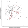 |
Fig. 2. Graphical representation of the PCA decomposition of the Shen sample in the EV1–EV2 plane, analogous to Fig. 1. |
2.3. PCA results of Boroson and Green for PG sample
For completeness, we also list in Table 2 the results from the original paper by Boroson & Green (1992). This sample contains 87 objects, for which 13 parameters were measured. We did not redo the analysis, but simply included the results given by Boroson & Green (1992) in their Table 4. In this sample the first two eigenvectors also dominate, although the effect is not as strong as in the reduced Shen sample.
3. Nonlinear analysis of the quasar main sequence
The quasar main sequence appears as a linear structure in the PCA analysis, since this method only allows for a linear analysis of the measured quantities. On the other hand, a strong impression of a 1D structure in the optical plane, defined by the Hβ FWHM and RFe II, is apparent (Sulentic et al. 2000; Marziani et al. 2018). There is an apparent steep decrease in Hβ FWHM as a function of RFe II at low values of RFe II, while a much shallower decrease is visible at high values. Following the results of the PCA analysis suggesting two dominant leading parameters, we attempted to define a new principal axis parameterized by a nonlinear decreasing curve in the FWHM(Hβ)–RFe II plane. As a test, we chose a simple decay curve that has two free parameters of the form shown in Eq. (1),
 (1)
(1)
where y and x are the Hβ FWHM and RFe II, respectively, while a and b are the free parameters. To find a and b we used the nls routine in R to find a fit to the reduced Shen datapoints on the plane. The plane, together with the resultant nonlinear fit, is shown in Fig. 3.
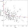 |
Fig. 3. Position of reduced Shen quasars (black dots) on the FWHM(Hβ)–RFe II plane. The decay curve is indicated in red. Blue diamonds indicate the boundaries of unit distance intervals along the curve after the axes are normalized to their respective sample means; the chosen zero point is shown first (uppermost center) and distance increasing toward the lower right. |
It is notable that the distribution of quasars in this high-quality sample looks distinctly different from that in Shen & Ho (2014) for the same plane. In that paper, the distribution is much more “triangular” (see their Fig. 1). In our distribution, it is better approximated by the decay curve. The path along the decay curve can be considered a nonlinear analog of the EV1 derived from PCA, while the EV2 would correspond to the perpendicular offset from the curve. We therefore transformed to a new coordinate plane parameterized by these new dimensions. This is achieved by first normalizing the Hβ FWHM and RFe II to their respective sample means and then finding the nearest point on the curve to each quasar data point (the “nearpoint”). Then, the two new parameters are assigned to each quasar data point.
The new principal parameter is defined by the distance along the curve, starting at the point where the mean-normalized Hβ FWHM is 2.5 (corresponding to 13 050 km s−1) and ending at each quasar nearpoint. This starting-point satisfies the requirement to have nonzero RFe II, since the curve becomes infinite at RFe II = 0. It is also just greater than the maximum Hβ FWHM in the quasar sample, and therefore is a suitable choice for the origin of the new main axis. The secondary parameter is therefore defined, for each quasar in the normalized plane, as the Euclidean distance from the quasar data point to the corresponding nearpoint.
If these new parameters indeed represent a plane analogous to EV1 and EV2 from PCA, then they should be linearly independent. However, a Spearman rank correlation test reveals a significant anticorrelation (probability of no correlation p = 0.03) between the new parameters across the sample. A visual examination of the plane in Fig. 3 suggests two outlying populations of five quasars at either end of the decay curve could be responsible. One group is those objects with FWHM(Hβ) > 10 500 km s−1, and another is those objects with RFe II > 1.2. With these outliers removed, the significant correlation disappears. The new plane is illustrated in Fig. 4, in which the removed outliers are highlighted. The five blue diamond markers in Fig. 3 correspond, in order from upper center to lower right, to the five indicated numerical values (0–4, respectively) on the horizontal axis of Fig. 4.
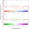 |
Fig. 4. Two panels showing the positions of the reduced Shen quasars (colored crosses) on the new plane, defined as indicated on the axis labels. Two groups of five outlying quasars are represented inside the ellipses at either end of the horizontal axis. Upper panel: crosses are color-coded by black hole masses obtained from the Shen catalog, while the lower panel crosses are color-coded by 3000 Å luminosity also obtained from Shen. The black hole mass units are log(M⊙) while luminosity units are log(erg cm−2 s−1 Å −1). |
4. Discussion
It is known from reverberation mapping (Blandford & McKee 1982) that AGN black hole mass scales with the Hβ FWHM, since the calculated masses (subject to the virial coefficient) are found to follow the M-σ relation determined for quiescent galaxies (Woo et al. 2010). This means the Eddington ratio should correlate negatively with Hβ FWHM, and indeed a significant anticorrelation between the two is found using a Spearman correlation test on the reduced Shen sample. We therefore ask if it is possible that the new principal parameter is measuring black hole mass. It would certainly be required that larger values of the new principal parameter indicate lower masses, given that this is the direction of lower Hβ FWHM. However it is also found that Eddington ratio tends to increase along the new principal parameter in the reduced sample. Therefore if this parameter is measuring black hole mass, it would require a decline in Eddington ratio at higher mass, possibly caused by the existence of a sub-Eddington limit (Steinhardt & Elvis 2010; Garofalo et al. 2019).
The conclusion that the black hole mass is the basic parameter changing along the quasar main sequence was formulated recently by Fraix-Burnet et al. (2017). They performed an analysis of two samples of 215 and 85 low-z quasars (z ≤ 0.7), using a machine learning approach in the form of an unsupervised multivariate classification technique. These authors included the measurement of seven independent parameters. This approach combines objects into trees according to the similarity of the parameters, and finally it can suggest an evolutionary pattern. The conclusion from their analysis was that the black hole mass, which grows over cosmological time, allows a reconstruction of the evolutionary pattern across the optical plane (see their Fig. 7). They interpret the effective coupling between mass and Eddington ratio as caused predominantly by the study of the local Universe, where sources that have both large black hole masses and high Eddington ratios are not present. This, in turn, is the result of galaxy evolution. Large black hole masses are hosted by large mass galaxies, as implied by the black hole mass–bulge mass correlation (Magorrian et al. 1998; de Nicola et al. 2019), and the gas content is relatively low with respect to the stellar mass in large galaxies. This last trend is already present at redshift ∼2, but it deepens with a redshift decrease, when the star formation rate and the gas content strongly decrease (see, e.g., Peeples & Shankar 2011; Popping et al. 2015; Decarli et al. 2019, and the references therein). Thus, the coupling is effectively due to limited resources of material in galaxies hosting increasingly massive black holes.
However, it is not entirely clear how a lower black hole mass (equivalently higher Eddington ratio in this case) could give rise to greater RFe II. A lower mass should produce a harder ionizing continuum, which would favor Hβ production over Fe II. A possible explanation for this is given in Marziani et al. (2018) based on different accretion disk modes. In this case when the Eddington ratio is high, the accretion disk behaves as a slim disk (Abramowicz et al. 1988), with “puffed up” walls close to the black hole. Conversely, at a low Eddington ratio, the disk behaves more like a traditional thin disk (Shakura & Sunyaev 1973). If this picture is true, low mass objects are likely to produce a flat, shielded region in which Fe II is preferentially formed over Hβ, thereby solving the puzzle.
We further inquired what would happen if the new secondary parameter in this case were luminosity. A correlation test indicates that this axis is strongly anticorrelated with luminosity, which is in accordance with the broad line region (BLR) radius-luminosity relationship determined in Kaspi et al. (2005). The slope of the decay curve indicates that the luminosity would have greater projection into RFe II as compared with Hβ FWHM at higher masses than at lower masses. Similar results have been obtained by Du & Wang (2019). This may be related to the difference in accretion disk mode. This is because at high masses differing luminosities could vary RFe II through ionization effects without getting close to Eddington luminosity owing to the sub-Eddington limit, while at low masses ionization effects are countered by the tendency of higher luminosity to create a greater shielded region in the slim disk regime.
It is likely that the Hβ FWHM is, to some degree, positively correlated with inclination angle, given the findings of studies that have used radio data as an orientation indicator (Wills & Brotherton 1995; Aars et al. 2005). This supports the idea of BLR Hβ emission originating in a flattened region, since at higher inclination the orbital velocity has greater projection into the plane of the line of sight. The study of Zamfir et al. (2008) showed that sources with Fanaroff–Riley type II (FR II) morphology are more common at higher Hβ FWHM than radio core-dominated sources. The FR II quasars are more likely to be viewed at high inclination as their radio lobes project into the plane of the sky as seen from Earth, further supporting the relationship between Hβ width and inclination.
It is also possible that RFe II declines with increasing orientation as Fe II is a relatively low ionization line and therefore may form in an even more flattened configuration than Hβ, since it necessitates shielding from the ionizing continuum. Indeed, evidence for this scheme is hinted at in Bisogni et al. (2017), where Fe II strength seems to drop to zero at very high [O III] EW (and hence inclination), while Hβ also drops but remains nonzero (see also Panda et al. 2019a,b). Given the shape of the decay curve in Fig. 3, it is therefore conceivable that the new main parameter anticorrelates with inclination angle. However even in such a case it is likely that mass plays a strong role because objects at low values of the new parameter predominantly have large line widths, which can only be achieved by high mass objects irrespective of inclination. It seems unlikely that inclination could form the main driver of the new secondary parameter, since increasing inclination should tend to increase the width of Hβ while suppressing the RFe II ratio (as discussed previously). An examination of Fig. 3 shows this is impossible, as all normal lines to the best-fit curve describe a change of both parameters in the same sense (positive or negative).
Another possibility is the involvement of black hole spin, however, for the BLR, this should mainly affect the hardness of the incident continuum, and higher spin results in a harder continuum. According to Panda et al. (2018), based on photoionization simulations, object-to-object variations in continuum peak temperature cannot explain the quasar main sequence. We can therefore say that it is most likely that the new principal parameter represents an anticorrelation with black hole mass, with the new secondary parameter representing an anticorrelation with luminosity. However, this does not rule out inclination having a separate influence on both Hβ FWHM and RFe II.
Outlying points. As can be seen in Fig. 4, the outlying points form two groups of five at either end of the new principal axis. It is worth considering the possible reasons these outliers exist. Studies of the quasar main sequence tend to show that the bulk of quasars are concentrated in the region 0 ≤ RFe II ≤ 1.0. This is also the case for our sample (see Fig. 3). It is not certain that values of RFe II greater than approximately 1.3 as derived from the Shen et al. (2011) catalog are accurate, since a more detailed investigation into a sample of such objects by Śniegowska et al. (2018) indicated that a large majority (21/27) did not have such a high value. This raises the possibility that the five outliers having the highest value of the new principal axis may be further from the bulk of quasars than warranted owing to an overestimation of RFe II. An example spectrum of one of these outliers is shown in Fig. 5.
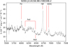 |
Fig. 5. Outlier represented in the right lower corner of Fig. 4. This quasar is an extreme representative of NLS1 class, with narrow Balmer lines and strong Fe II emission, but otherwise it does not show any peculiarities in the spectrum. |
Any miscalculation of RFe II or Hβ FWHM in Shen et al. (2011) would result from inaccurate modeling of one or both of the Fe II and Hβ emissions. Accurate determination of the strength and shape of the emission profiles strongly depends on correct placement of the disk continuum, which is difficult in a spectral region heavily contaminated by line emission. Also, the Fe II blend spans approximately 4340 Å–4680 Å, which overlaps with the broad He II emission at 4686 Å. It thus may be difficult to distinguish between the two and, as a result, the He II flux in this region might be wrongly attributed to Fe II or vice versa. In cases of very large width the Hβ line itself could overlap with the Fe II blend as seen, for example, in Fig. 6 of Marziani & Sulentic (2012), resulting in confusion between the two.
For the group with low values of the new principal axis, it is possible that the true Hβ kinematic line width is overestimated, pushing them away from the quasar bulk. This may result from variable asymmetric broad emission line caused by complexities such as shocks generating emission in addition to photoionization (Shapovalova et al. 2010). From examination of the Hβ profiles in these objects, this explanation is indeed plausible, as they appear to have a characteristic double-peaked profile. An example spectrum where this phenomenon is visible is shown in Fig. 6.
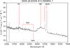 |
Fig. 6. Extreme outlier in the center upper corner of Fig. 4. This quasar and neighboring outliers are characterized by the double-peak profile of the broad component of Hβ line. |
The offset of the broad component centroid of Hβ from the theoretical quasar rest-frame wavelength can also give clues regarding the nature of the outlying points. Asymmetries can result in large offsets, and these asymmetries can either be intrinsic or artifacts of incorrectly modeled profiles. In Fig. 7 the Hβ widths and offsets are listed for all quasars in the reduced Shen sample, with both sets of outliers highlighted. As can be seen, larger offsets generally result from broader lines. The fraction of non-outlying points with offsets placing them outside the mean envelop (61 out of 165 or 37%) is smaller than that of outlying points (6 out of 10 or 60%). This could indicate that one of the previously mentioned mechanisms may be responsible for the outliers. The object with an offset of −3670 km s−1 appears extreme in this plot and therefore is of note, however upon inspection the spectrum did not appear unusual.
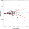 |
Fig. 7. Widths and Hβ offsets of the reduced Shen quasars (black diamonds). Outlying points are shown as cyan for low principal axis values and magenta for high principal axis values. Red lines indicate an envelope calculated from a five-point moving magnitude average. |
5. Conclusions
We have shown, for a high-quality quasar sample, that it is possible to describe the behavior of the quasar main sequence in the FWHM(Hβ)–RFe II plane using two linearly independent parameters, as suggested by the PCA analysis. One of these is distance along a decay curve, which accounts for the majority of variance, and the other is the distance in parameter space of each object from the curve. The distribution of quasar data points in the FWHM(Hβ)–RFe II plane is distinctly different from that of Shen & Ho (2014), which is approximately triangular.
If the two new parameters dominate the behavior of the quasar main sequence, then we can suggest what they may be. Given the already well-known positive relationship between Hβ width and black hole mass, together with the additional possibility of RFe II dependence on accretion disk mode and shielding effects, it seems very plausible that the distance along the decay curve represents the direction of decreasing black hole mass. In this case the secondary axes would probably represent luminosity. The effect of inclination on Hβ FWHM however is strongly suggested by previous studies, so it probably has an influence, even if it is not one of the primary drivers of the new parameters.
Acknowledgments
The project was partially supported by Polish grant No. 2015/17/B/ST9/03436/.
References
- Aars, C. E., Hough, D. H., Yu, L. H., et al. 2005, AJ, 130, 23 [NASA ADS] [CrossRef] [Google Scholar]
- Abramowicz, M. A., Czerny, B., Lasota, J. P., & Szuszkiewicz, E. 1988, ApJ, 332, 646 [NASA ADS] [CrossRef] [Google Scholar]
- Bisogni, S., Marconi, A., & Risaliti, G. 2017, MNRAS, 464, 385 [NASA ADS] [CrossRef] [Google Scholar]
- Blandford, R. D., & McKee, C. F. 1982, ApJ, 255, 419 [NASA ADS] [CrossRef] [EDP Sciences] [Google Scholar]
- Boroson, T. A., & Green, R. F. 1992, ApJS, 80, 109 [NASA ADS] [CrossRef] [Google Scholar]
- Capellupo, D. M., Netzer, H., Lira, P., Trakhtenbrot, B., & Mejía-Restrepo, J. 2015, MNRAS, 446, 3427 [NASA ADS] [CrossRef] [Google Scholar]
- Capellupo, D. M., Netzer, H., Lira, P., Trakhtenbrot, B., & Mejía-Restrepo, J. 2016, MNRAS, 460, 212 [NASA ADS] [CrossRef] [Google Scholar]
- Collin, S., Kawaguchi, T., Peterson, B. M., & Vestergaard, M. 2006, A&A, 456, 75 [NASA ADS] [CrossRef] [EDP Sciences] [Google Scholar]
- de Nicola, S., Marconi, A., & Longo, G. 2019, MNRAS, 490, 600 [NASA ADS] [CrossRef] [Google Scholar]
- Decarli, R., Walter, F., Gónzalez-López, J., et al. 2019, ApJ, 882, 138 [NASA ADS] [CrossRef] [Google Scholar]
- Du, P., & Wang, J.-M. 2019, ApJ, submitted [arXiv:1909.06735] [Google Scholar]
- Fraix-Burnet, D., Marziani, P., D’Onofrio, M., & Dultzin, D. 2017, Front. Astron. Space Sci., 4, 1 [NASA ADS] [Google Scholar]
- Garofalo, D., Christian, D. J., & Jones, A. M. 2019, Universe, 5, 145 [NASA ADS] [CrossRef] [Google Scholar]
- Kaspi, S., Maoz, D., Netzer, H., et al. 2005, ApJ, 629, 61 [NASA ADS] [CrossRef] [Google Scholar]
- Kuraszkiewicz, J., Wilkes, B. J., Schmidt, G., et al. 2009, ApJ, 692, 1180 [NASA ADS] [CrossRef] [Google Scholar]
- Magorrian, J., Tremaine, S., Richstone, D., et al. 1998, AJ, 115, 2285 [NASA ADS] [CrossRef] [Google Scholar]
- Marziani, P., & Sulentic, J. W. 2012, New Astron. Rev., 56, 49 [NASA ADS] [CrossRef] [Google Scholar]
- Marziani, P., Sulentic, J. W., Zwitter, T., Dultzin-Hacyan, D., & Calvani, M. 2001, ApJ, 558, 553 [NASA ADS] [CrossRef] [Google Scholar]
- Marziani, P., Del Olmo, A., D’Onofrio, M., & Dultzin, D. 2018, Front. Astron. Space Sci., 5, 28 [NASA ADS] [CrossRef] [Google Scholar]
- Matt, G., Maiolino, R., & Guainazzi, M. 2003, MNRAS, 342, 422 [NASA ADS] [CrossRef] [Google Scholar]
- Mejía-Restrepo, J. E., Trakhtenbrot, B., Lira, P., Netzer, H., & Capellupo, D. M. 2016, MNRAS, 460, 187 [NASA ADS] [CrossRef] [Google Scholar]
- Panda, S., Czerny, B., Adhikari, T. P., et al. 2018, ApJ, 866, 115 [NASA ADS] [CrossRef] [Google Scholar]
- Panda, S., Marziani, P., & Czerny, B. 2019a, ArXiv e-prints [arXiv:1908.07972] [Google Scholar]
- Panda, S., Marziani, P., & Czerny, B. 2019b, ApJ, 882, 79 [NASA ADS] [CrossRef] [Google Scholar]
- Peeples, M. S., & Shankar, F. 2011, MNRAS, 417, 2962 [NASA ADS] [CrossRef] [Google Scholar]
- Peterson, B. M. 1997, An Introduction to Active Galactic Nuclei (Cambridge: Cambridge University Press) [CrossRef] [Google Scholar]
- Popping, G., Behroozi, P. S., & Peeples, M. S. 2015, MNRAS, 449, 477 [NASA ADS] [CrossRef] [Google Scholar]
- Risaliti, G., Salvati, M., & Marconi, A. 2011, MNRAS, 411, 2223 [NASA ADS] [CrossRef] [Google Scholar]
- Shakura, N. I., & Sunyaev, R. A. 1973, A&A, 24, 337 [NASA ADS] [Google Scholar]
- Shapovalova, A. I., Popović, L. Č., Burenkov, A. N., et al. 2010, A&A, 509, A106 [NASA ADS] [CrossRef] [EDP Sciences] [Google Scholar]
- Shen, Y., & Ho, L. C. 2014, Nature, 513, 210 [NASA ADS] [CrossRef] [Google Scholar]
- Shen, Y., Richards, G. T., Strauss, M. A., et al. 2011, ApJS, 194, 45 [NASA ADS] [CrossRef] [Google Scholar]
- Śniegowska, M., Czerny, B., You, B., et al. 2018, A&A, 613, A38 [NASA ADS] [CrossRef] [EDP Sciences] [Google Scholar]
- Steinhardt, C. L., & Elvis, M. 2010, MNRAS, 402, 2637 [NASA ADS] [CrossRef] [Google Scholar]
- Sulentic, J. W., Zwitter, T., Marziani, P., & Dultzin-Hacyan, D. 2000, ApJ, 536, L5 [NASA ADS] [CrossRef] [Google Scholar]
- Sulentic, J. W., Bachev, R., Marziani, P., Negrete, C. A., & Dultzin, D. 2007, ApJ, 666, 757 [NASA ADS] [CrossRef] [Google Scholar]
- Wills, B. J., & Brotherton, M. S. 1995, ApJ, 448, L81 [NASA ADS] [CrossRef] [Google Scholar]
- Woo, J.-H., Treu, T., Barth, A. J., et al. 2010, ApJ, 716, 269 [NASA ADS] [CrossRef] [Google Scholar]
- Zamfir, S., Sulentic, J. W., & Marziani, P. 2008, MNRAS, 387, 856 [NASA ADS] [CrossRef] [Google Scholar]
All Tables
All Figures
|
Fig. 1. Graphical representation of the PCA decomposition of the Capellupo sample reduced to 13 parameters. The dots represent individual objects on the standardized EV1–EV2 plane that have values indicated by the axis labels. The arrows represent the loadings of the variables in the EV1–EV2 plane; the unit circle is included for scale reference. |
| In the text | |
|
Fig. 2. Graphical representation of the PCA decomposition of the Shen sample in the EV1–EV2 plane, analogous to Fig. 1. |
| In the text | |
|
Fig. 3. Position of reduced Shen quasars (black dots) on the FWHM(Hβ)–RFe II plane. The decay curve is indicated in red. Blue diamonds indicate the boundaries of unit distance intervals along the curve after the axes are normalized to their respective sample means; the chosen zero point is shown first (uppermost center) and distance increasing toward the lower right. |
| In the text | |
|
Fig. 4. Two panels showing the positions of the reduced Shen quasars (colored crosses) on the new plane, defined as indicated on the axis labels. Two groups of five outlying quasars are represented inside the ellipses at either end of the horizontal axis. Upper panel: crosses are color-coded by black hole masses obtained from the Shen catalog, while the lower panel crosses are color-coded by 3000 Å luminosity also obtained from Shen. The black hole mass units are log(M⊙) while luminosity units are log(erg cm−2 s−1 Å −1). |
| In the text | |
|
Fig. 5. Outlier represented in the right lower corner of Fig. 4. This quasar is an extreme representative of NLS1 class, with narrow Balmer lines and strong Fe II emission, but otherwise it does not show any peculiarities in the spectrum. |
| In the text | |
|
Fig. 6. Extreme outlier in the center upper corner of Fig. 4. This quasar and neighboring outliers are characterized by the double-peak profile of the broad component of Hβ line. |
| In the text | |
|
Fig. 7. Widths and Hβ offsets of the reduced Shen quasars (black diamonds). Outlying points are shown as cyan for low principal axis values and magenta for high principal axis values. Red lines indicate an envelope calculated from a five-point moving magnitude average. |
| In the text | |
Current usage metrics show cumulative count of Article Views (full-text article views including HTML views, PDF and ePub downloads, according to the available data) and Abstracts Views on Vision4Press platform.
Data correspond to usage on the plateform after 2015. The current usage metrics is available 48-96 hours after online publication and is updated daily on week days.
Initial download of the metrics may take a while.