| Issue |
A&A
Volume 631, November 2019
|
|
|---|---|---|
| Article Number | A89 | |
| Number of page(s) | 10 | |
| Section | Planets and planetary systems | |
| DOI | https://doi.org/10.1051/0004-6361/201936600 | |
| Published online | 25 October 2019 | |
On the inclinations of the Jupiter Trojans
Lund Observatory, Department of Astronomy and Theoretical Physics, Lund University,
Box 43,
22100
Lund,
Sweden
e-mail: This email address is being protected from spambots. You need JavaScript enabled to view it.
Received:
29
August
2019
Accepted:
3
October
2019
Abstract
Jupiter Trojans are a resonant asteroidal population characterised by photometric colours that are compatible with trans-Neptunian objects, high inclinations, and an asymmetric distribution of the number of asteroids between the two swarms. Different models have been proposed to explain the high inclination of the Trojans and to interpret their relation with the Trans-Neptunian objects, but none of these models can also satisfactorily explain the asymmetry ratio between the number of asteroids in the two swarms. It has recently been found that the asymmetry ratio can arise if Jupiter has migrated inwards through the protoplanetary disc by at least a few astronomical units during its growth. The more numerous population of the leading swarm and the dark photometric colours of the Trojans are natural outcomes of this new model, but simulations with massless unperturbed disc particles led to a flat distribution of the Trojan inclinations and a final total mass of the Trojans that was 3–4 orders of magnitude larger than the current mass. We here investigate the possible origin of the peculiar inclination distribution of the Trojans in the scenario where Jupiter migrates inwards. We analyse different possibilities: (a) the secular evolution of an initially flat Trojan population, (b) the presence of planetary embryos among the Trojans, and (c) capture of the Trojans from a pre-stirred planetesimal population in which Jupiter grows and migrates. We find that the secular evolution of the Trojans and secular perturbations from Saturn do not affect the inclination distribution of the Trojans appreciably, nor is there any significant mass depletion over the age of the Solar System. Embryos embedded in the Trojan swarms, in contrast, can stir the Trojans to their current degree of excitation and can also deplete the swarms efficiently, but it is very difficult to remove all of the massive bodies in 4.5 Gyr of evolution. We propose that the disc where Jupiter’s core was forming was already stirred to high inclination values by other planetary embryos competing in the feeding zone of Jupiter’s core. We show that the trapped Trojans preserve their high inclination through the gas phase of the protoplanetary disc and that Saturn’s perturbations are more effective on highly inclined Trojans, leading to a lower capture efficiency and to a substantial depletion of the swarms during 4.5 Gyr of evolution.
Key words: minor planets, asteroids: general / planets and satellites: dynamical evolution and stability
© ESO 2019
1 Introduction
Jupiter Trojans are a population of minor bodies in our Solar System. They share the same orbit of Jupiter, that has a semimajor axis of about 5.2 au, and cluster in two different regions along its orbit. The leading group precedes Jupiter and librates around the L4 triangular Lagrangian point, and the trailing group follows Jupiter and librates around the L5 triangular Lagrangian point. The number of asteroids in the leading group is larger than that of the trailing group, which is measured as an asymmetry ratio between the two swarms of 1.4 ± 0.2 for Trojans larger than 10 km (Grav et al. 2011). The Trojan orbits have high inclinations (up to 40°) and are very dark objects, more similar to trans-Neptunian objects (TNOs) than to asteroid belt objects. They are mainly D-type asteroids (very low albedo and relatively featureless spectra with a very steep red slope) with a few P-type (low-albedo and featureless spectrum with reddish slope) and C-type (also low albedo and carbon rich) asteroids (Barucci et al. 2002; DeMeo & Carry 2014) in contrast to the main belt objects.
Jupiter Trojans could represent the key to understanding the formation and evolution of the early Solar System. Their peculiar characteristics, such as the asymmetry ratio, the high-inclination distribution, and the predominance of D- and P-type asteroids among them, must be explained in order to unveil the history of Jupiter and thus the history of the entire Solar System.
One of the most plausible hypotheses for the origin of Jupiter Trojans is the so-called “chaotic capture” (Morbidelli et al. 2005): any primordial Trojan is lost during the late instability of the giant planets (Morbidelli et al. 2005; Tsiganis et al. 2005; Gomes et al. 2005) as Jupiter and Saturn cross their mutual 2:1 mean motion resonance. The swarms are then refilled with TNOs that are destabilised by the outward migration of Neptune. TNOs are very dark objects and those that are captured as Trojans also have a high-inclination distribution. Despite successfully matching these features, the model suffers from a low capture probability of between 10−6 and 10−5 (Lykawka & Horner 2010), and it provides no explanation for the asymmetry ratio between the two Trojan swarms.
In the “jump capture” (Nesvorný et al. 2013), a fifth giant planet in the very early Solar System is instead invoked. According to this model, Jupiter had multiple close encounters with this additional planet when the system became unstable. As a result, the semimajor axis of Jupiter jumps and radially displaces the Trojan stable regions, losing the primordial Trojans and capturing new asteroids with semimajor axes similar to its new position. At the time of the last jump of Jupiter’s semimajor axis (i.e., when Trojans are captured), the vicinity of the planet was populated with TNOs destabilised by the outwardmigration of Neptune. This model reproduces the orbital distribution of the Trojans and their dark photometriccolour, and it is also potentially capable of explaining their asymmetry ratio: when the additional ice giant involved in the planet–planet scattering with Jupiter traverses one of the Trojan swarms, it can scatter captured bodies out of the stable region, which depletes the swarm. However, even if the additional ice giant traverses the correct swarm, the results in Nesvorný et al. (2013) cannot rule out a symmetric ratio between the swarms within 1σ. The low capture probability, of the order of 6−8 × 10⁻⁷, is another weakness in this model as well.
Recently, Pirani et al. (2019) showed that the asymmetry ratio of the Trojans could arise as a direct consequence of the early inward migration of Jupiter through the gaseous protoplanetary disc phase while it was growing to become a gas giant. In this scenario, Jupiter’s core grows according to the core accretion model (Pollack et al. 1996) boosted by pebble accretion (Johansen & Lacerda 2010; Ormel & Klahr 2010; Lambrechts & Johansen 2012; Ida et al. 2016; Johansen & Lambrechts 2017) and migrates inwards due to interactions with the gaseous disc (Ward 1997; Lin & Papaloizou 1986), following growth tracks similar to those shown in Bitsch et al. (2015). In order for Jupiter to end its inward migration at about 5 au when the gaseous disc disperses, its core has to form in the outer Solar System. Trojans are captured in the feeding zone of Jupiter’s core, at about 20 au, among objects that naturally posses dark photometric colours, and then are dragged by the migrating planet to where they currently orbit. The relative drift between the planet and the Trojans induces a deformationof the horseshoe orbits of asteroids in resonance with Jupiter, leading to an excess of objects in the L4 side of the horseshoe region. The mass growth of Jupiter then shrinks these orbits into tadpole orbits, which causes the asymmetry. Despite this good agreement with observations, the simulations of Pirani et al. (2019) showed a final mass of the Trojans that is 3–4 orders of magnitude higher than the current mass and an inclination distribution that is much flatter than the current distribution.
The high-inclination distribution of the Trojans is a long-standing problem in the models where Trojans are captured from planetesimals orbiting in the vicinity of Jupiter during its growth, the so-called “local capture models” (Marzari et al. 2002). Different solutions have been proposed to drive them into high-inclination orbits: the raising of inclinations by secular resonances (Marzari & Scholl 2000); a process analogous to that suggested by Wetherill (1992) and Petit et al. (2001), that is, to posit the presence of the massive embryos in the Trojan swarms that excited the population by their gravity and were ejected from the stable regions by mutual perturbations; and the possibility that Trojans were stirred up prior to capture by proto-Jupiter, as suggested in Marzari et al. (2002).
The aim of this follow-up paper is to address the Trojan mass and inclination problems identified in Pirani et al. (2019). In order to do this, we explore three different plausible ways to incline the Trojans up to 40° and keep track of the mass depletion in each different scenario. Under the influence of Jupiter and Saturn, we here test three scenarii: (a) the secular evolution of an initially flat Trojan population, (b) the presence of massive planetary embryos among the Trojans, and (c) a pre-stirred disc planetesimal population in which Jupiter grows and migrates.
The paper is organised as follows: in Sect. 2 we describe the different scenarios and methods used in our simulations, and in Sect. 3 we present our results. Finally, in Sect. 4 we summarise our results and discuss their implications.
2 Methods
In our simulations, we used a parallelised version of the MERCURY N-body code (Chambers 1999), and we selected its hybrid symplectic integrator, which is faster than conventional N-body algorithms by about one order of magnitude (Wisdom & Holman 1991). It is particularly suitable for our simulations, which involve timescales of the order of billions of years. We used a time step of 140 days, that is, about 1/20 of the orbital period of a particle orbiting at about 4 au (Duncan et al. 1998). Because we are interested in the Trojans that orbit with Jupiter at 5.2 au, this is a sufficient resolution. We modified the code so that the giant planets grow and migrate according to the growth tracks generated following the recipes in Johansen & Lambrechts (2017), as we explain in Sect. 2.1.
In the MERCURY N-body code, the planets and planetary embryos are treated as massive bodies, so that they perturb and interact with all the other bodies during the integration. The other particles, called small bodies, are perturbed by the massive bodies, but cannot affect each other. Because we set them as massless, they cannot perturb the massive bodies either. We refer to these particles in the text as massless particles or small bodies. In our simulations we used these massless particles to populate the protoplanetary disc in which Jupiter grows and migrates. Our version of the code also includes aerodynamic gas drag effects and tidal gas drag effects to mimic the presence of the gas in the protoplanetary disc as in Pirani et al. (2019). The growing protoplanets and planetary embryos are affected by the tidal gas drag, and the massless particles are affected by the aerodynamic gas drag until the gaseous protoplanetary disc photoevaporates at t = 3 Myr, according to typical disc lifetimes (Mamajek 2009; Williams & Cieza 2011). Because small bodies are set to be massless during the integrations, we assigned them a radius rp = 50 km and a density ρp = 1.0 g cm−3 when we computed the effect of the aerodynamic gas drag on the particle, that is, the typical size resulting from streaming instability simulations (Johansen et al. 2014).
A key result from Pirani et al. (2019) is that Jupiter Trojans are almost all captured from the feeding zone of Jupiter’s core. Because of this, our massless particle disc extends only for about ±2.5 au from the location of Jupiter’s core. The disc is then divided into annular regions of 0.5 au, populated by 10 000 massless particles each. The same number of particles in each annular region means that we adopted a surface density proportional to r−1 for the primordial bodies component.
2.1 Growth tracks
In order to generate the growth tracks for Jupiter and Saturn that we implemented in our simulations, we used therecipes in Johansen & Lambrechts (2017). The disc parameters for our model were fg =0.2, fp =0.4, fpla = 0.2, H∕r = 0.04, Hp /H = 0.1, Δv = 30 m s−1 and St = 0.1, where fg, fp, and fpla are parameterisations of the column densities (of the gas, pebbles, and planetesimals, respectively) relative to the standard profiles, H∕r is the disc aspect ratio, Hp ∕H is the particle midplane layer thickness ratio, Δv is the sub-Keplerian speed of the gas slowed down by the radial pressure support, and St is the Stokes number of the pebbles. The growth tracks of Jupiter and Saturn are shown in Fig. 1. The initial mass of the Jupiter seed is 10−2 M⊕ and its final mass is about 300M⊕. It migrates from 18 au to its current orbit at 5.2 au. The migration starts at about 2.2 Myr and stops when the gas dissipates at 3 Myr. The growth track of Saturn is similar to that of Jupiter. Saturn starts as massive as the Jupiter seed (10−2 M⊕) and reaches a final mass of 95 M⊕. It migrates from 21 to 9.5 au in about 0.8 Myr.
We did not simulate any late instability of the giant planets as in the Nice Model (Morbidelli et al. 2005; Tsiganis et al. 2005; Gomes et al. 2005) and the fifth giant planet model (Nesvorný 2011), nor did we lock the planets in any mutual resonances. Timescales and the time when the late instability occurs are still debated (Morbidelli et al. 2018), as is the time (if any) that the planets spend in mean motion resonance. The amount of depletion to be attributed to the late instability highly depends on which version we consider, and we do not explore it in this paper. Pirani et al. (2019) showed that Trojans and their original asymmetry can survive a single jump of Jupiter of 0.2 au. In line with this, we attributed a fictitious 80% of depletion of the Trojans to the late instability when we analysed our results. We did not include the so-called Grand Tack (Walsh et al. 2011) hypothesis either, where Jupiter is assumed to migrate inwards in the inner Solar System, deep to about 1.5 au, before Saturn (also migrating inwards) is caught in a 2:3 mean-motion resonance with it. At this point, the migration of Jupiter changes direction and the giant planets move outwards, which explains the mixing, the excitation, the depletion of the main asteroid belt, and the low mass of Mars. Because we did not focus on the asteroid belt and because a slightly deeper migration does not alter our results on the Trojans significantly, we proceeded with the scenario in which Jupiter reaches 5.2 au when the protoplanetary disc photoevaporates at 3 Myr.
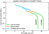 |
Fig. 1 Growth tracks of Jupiter and Saturn. The gas giants start with an initial mass of 10−2 M⊕ and grow to their current mass. Jupiter migrates from 18 au to its current orbit at 5.2 au and Saturn migrates from 21 au to 9.5 au. The migration starts at ~2.2 Myr and stops when the gas dissipates at 3 Myr. The green solid line corresponds to the core accretion phase, the orange solid line corresponds to the gas accretion phase, and the cyan solid line corresponds to the runaway gas accretion phase. |
2.2 Secular evolution of massless Trojans
In the first set of simulations, we generated massless particles with random eccentricities in the interval [0, 0.01], random inclinations in the interval [0°, 0.01°], and random semimajor axes in each Δa = 0.5 au annular region. We used a flat inclination distribution for our unperturbed disc particles. In each annular region we placed 104 massless particles from 15.5 to 20.5 au for a total of 105 particles. As shown in Fig. 1, Jupiter’s core starts at 18 au, therefore we placed it exactly in the middle of the particle disc. We called J0 the simulation when only Jupiter is present, and JS0 the simulation when Saturn is also added to the system.
Jupiter grows and migrates following the growth track in Fig. 1 and traps a Trojan population compatible in mass and inclination distribution with the Trojans reported in Pirani et al. (2019). We analysed both the case with only Jupiter, where the final configuration is Jupiter at 5.2 au with a circular orbit and zero inclination, and the case with Jupiter plus Saturn, where we let the two giant planets migrate to their current orbits and artificially smoothly increased their inclination and eccentricity to their current values following the exponential laws present in Pirani et al. (2019) with an e-folding time of τ = 5 Myr. The starting inclination distribution of the Trojans was evaluated at 5 Myr, which is 2 Myr after Jupiter reaches its current semimajor axis because we wished to avoid counting eccentric interlopers stirred by the migration as Trojans. Figure 2 shows the initial Trojan inclinations for simulations J0 (in blue) and JS0 (in red). The grey histogram represents the current inclination distribution of Jupiter Trojans. As expected from the results in Pirani et al. (2019), the distributions remain very flat after the large-scale migration and growth of the giant planet. This is because inward migration and mass growth of Jupiter do not affect Trojan inclinations because they are quasi-invariant under mass growth and migration of the gas giant (Fleming & Hamilton 2000).
The starting number of Trojans, the mass, and the asymmetry ratio for simulations J0 and JS0 are summarised in Table 1. In order to estimate the initial mass, we considered the minimum mass solar nebula (MMSN; Weidenschilling 1977; Hayashi 1981), which predicts approximately 1 M⊕ of mass in each annular region of one astronomical unit. Because we have 10 000 particles in each 0.5 annular region, a massless particle in our simulations represents 5 × 10⁻⁵ M⊕. We are aware that the MMSN model cannot be too accurate because the planets migrate through the disc during their formation, but our main purpose is to assess the mass depletion as a relative value to the initial mass, and not the absolute value, in the different scenarios.
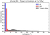 |
Fig. 2 Starting inclinations for J0 (blue histogram) and JS0 (red histogram) at 5 Myr. The grey histogram represents the current inclination distribution of Jupiter Trojans. |
Initial Trojan populations in J0 and JS0 simulations at t = 5 Myr.
2.3 Embryos embedded in the Trojan swarms
In this second scenario, we take advantage of the Trojan population trapped in cases of the flat particle disc that we discussed in Sect. 2.2. Of the resulting initial Jupiter Trojans of the previous set of simulations, at t = 5 Myr we substituted part of them in the MERCURY N-body code as massive bodies according to the size frequency distribution obtained from the planetesimal formation simulations of Schäfer et al. (2017) and restarted a second separate set of simulations. The size frequency distribution is consistent with an exponentially tapered power law with an exponential cutoff at the high-radius end:
![Mathematical equation: \begin{equation*} \frac{N_>(R)}{N_{\textrm{tot}}}=\left(\frac{R}{R_{\textrm{min}}}\right)^{-3{\alpha}}\exp\left[\left(\frac{R_{\textrm{min}}}{R_{\textrm{exp}}}\right)^{3{\beta}}-\left(\frac{R}{R_{\textrm{exp}}}\right)^{3{\beta}}\right]. \end{equation*}](/articles/aa/full_html/2019/11/aa36600-19/aa36600-19-eq1.png) (1)
(1)
Here N>(R) is the number of Trojans with radius greater than R, where R is the radius of each Trojan. Ntot is their total number, Rmin is the minimum Trojan radius, and Rexp is the exponential cutoff radius. α is the power-law exponent of the exponentially tapered power law, and β is the steepness of the exponential cutoff. We set Ntot in order to approximately represent the total initial mass of the Trojans estimated with the MMSN model that is reported in Table 1, α = 0.6 and β = 0.35.
2.3.1 More and less massive embryos
For Rmin and Rexp, we simulated two different distributions:
- (i)
Rmin = 100 km and Rexp = 250 km, where the most massive Trojan of the distribution has a mass of 2 × 10⁻³ M⊕ (Pluto-like bodies).
- (ii)
Rmin = 10 km and Rexp = 100 km, consistent with characteristic radii inferred for TNOs (Abod et al. 2019), where the most massive Trojan has a mass of 3 × 10⁻⁴ M⊕ (Ceres-like bodies).
The size frequency distributions in the two different cases are shown in Fig. 3. The top histogram represents the case with Rmin = 100 km and Rexp = 250 km, and the bottom histogram represents the case with Rmin = 10 km and Rexp = 100 km. Because the total mass is the same, but the range of the object sizes of the distributions is different, the total number of asteroids in the two cases differs. The black arrow in the figures indicates the mass of asteroid (624) Hektor of about 7.9 × 10¹⁸ kg (Marchis et al. 2014), which is the most massive Jupiter Trojan. For reasons of computational time, we substituted just the most massive part of the distribution into the Trojan population and we indicate it in cyan; in blue we show the remaining size frequency distribution that we did not consider. In the case of Rmin = 100 km and Rexp = 250 km, we substituted 86 bodies, and in the case of Rmin = 10 km and Rexp = 100 km, we substituted 63 bodies. These numbers depend on the logarithmic bins we used in between the intervals Rmin and Rmax, where Rmax is the maximum size of the distribution.
For this second set of simulations, we also considered the case of Jupiter migrating alone and the case in which Saturn migrates together with it. We called the simulations where only Jupiter migrates J100 and J250, with Rexp = 100 km and Rexp = 250 km values for the exponential cutoff radius, respectively. JS100 and JS250 are the simulations in which Saturn is added to the system, with Rexp = 100 km and Rexp = 250 km values for the exponential cutoff radius, respectively. We substituted the particles in a completely arbitrary way: we substituted the first 86 (or 63) first massless particles in the input file with massive embryos without knowing if the substituted particle belongs to the L4 or L5 swarm because in the file they are ranked by their initial position in the disc and hence in a random order. Simulations stopped at t = 4.5 Gyr, and we assessed the depletion history of the swarms, the fate of the embryos embedded in the swarms, and whether the asymmetry is sensitive to the presence of embryos.
2.3.2 Loss of the embryos from the Trojan swarms
The previous type of simulations, with almost one hundred massive bodies, is computationally very expensive even when we only try to include just a small part of the distribution as massive bodies. We decided to run an additional subset of ten simulations in which we substituted just the ten most massive bodies from the distribution with Rmin = 10 km and Rexp = 100 km. We called these simulations 10EMBRYOS. We considered only the case when both Jupiter and Saturn migrated. The aim of these simulations was to try to understand if it is easy to lose the massive Trojans from both swarms. We arbitrarily substituted the massive bodies here as well, regardless of whether they belonged to the L4 or L5 swarm. The startingdistribution of the massive embryos within the two swarms is reported in Table 5 together with the results after t = 4.5 Gyr.
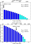 |
Fig. 3 Size frequency distributions of the Jupiter Trojans in the case of Rmin = 100 km and Rexp = 250 km (top histogram) and for Rmin = 10 km and Rexp = 100 km (bottom histogram). The histograms show the number of Trojans in mass bins (bottom x-axis). In the upper x-axes we show the correspondent radius bins (we assumed a density of the Trojans of 1.5 g cm−3). In cyan we highlight the part of the distributions that we substituted into the Trojan swarms as massive bodies. The black arrow indicates the mass of asteroid (624) Hektor, which is the most massive Jupiter Trojan. |
2.4 Pre-stirred planetesimal disc
In the third and final scenario, we started with a disc that was pre-stirred before the capture of Trojans by proto-Jupiter (Kokubo & Ida 2000). We used two different distributions for the initial inclination and eccentricity: in the first case we used the current inclination and eccentricity distribution of the main asteroid belt, which is thought to have been depleted and excited by the presence of planetary embryos (Wetherill 1992; Petit et al. 1998; Chambers & Wetherill 2001; Petit et al. 2001; Bottke et al. 2005; O’Brien et al. 2007). As modelled in Minton & Malhotra (2010), the initial eccentricity distribution of the disc particles can be modelled as a Gaussian with the peak at μe = 0.15, a standard deviation σe = 0.07, and a lowercutoff at zero. The initial inclination distribution is a Gaussian with the peak at μi = 8.5°, a standard deviation σi = 7°, and a lower cutoff at 0°. We called the simulation with only Jupiter JPRESTIRRED_AB and the simulation that also included Saturn JSPRESTIRRED_AB, where “ab” stands for asteroid belt. The initial inclination distribution of the particles in this case is shown in the top histogram of Fig. 4. In the second case, we used the current inclination and eccentricity distribution of the classical Kuiper Belt objects (CKBOs), that is, hot classicals (HCs) plus cold classicals (CCs). We modelled them as in Volk & Malhotra (2011) to a sum of two Gaussians. The initial inclination distribution is shown in the bottom histogram of Fig. 4. We called these simulations JPRESTIRRED_CKBO when only Jupiter migrates and JSPRESTIRRED_CKBO when Saturn is included. In the same way as for the first two scenarios, we ran the simulations for t = 4.5 Gyr in order to assess the capture efficiency of the Trojans compared to the flat disc case, the depletion history of the swarms, and the asymmetry evolution, if any.
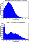 |
Fig. 4 In the JPRESTIRRED_AB and JSPRESTIRRED_AB simulations we used an inclination distribution model similar to the asteroid belt distribution (top histogram). In the JPRESTIRRED_CKBO and JSPRESTIRRED_CKBO simulations we used an inclination distribution model similar to the CKBOs distribution (bottom histogram). |
3 Results
3.1 Secular evolution of Jupiter Trojans with a flat inclination distribution (J0 and JS0)
The results of J0 and JS0 are summarised in Table 2. In the J0 simulation, Jupiter Trojans are very stable over an evolution of t = 4.5 Gyr when Jupiter alone is present in the system. This means that there is no mass depletion over the history of the Solar System and that the original asymmetry ratio between the number of Trojans in L4 and L5 is also preserved. In the scenario that includes both Jupiter and Saturn, we note that interactions between the two planets during the migration led to a lower capture efficiency. The JS0 simulation reports 15% less Trojans as captured (2208 captured Trojans in JS0 compared with 2600 in J0). Moreover, when the planets cease migrating, the depletion of the Jupiter Trojan swarms continues, as shown in the fourth column of Table 2. The depletion is of the order of 40% over an evolution of 4.5 Gyr. The inclination distributions for the final orbital parameters of the Trojans after an evolution of 4.5 Gyr are shown in Fig. 5. In both scenarios, with and without Saturn, the inclination distribution of the Jupiter Trojans remains very flat through the t = 4.5 Gyr we integrated. These results disagree with the current Trojan inclinations, which are up to 40°.
Evolution of the number of Trojans, their total mass, and the asymmetry ratio for simulations J0 and JS0.
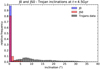 |
Fig. 5 Inclination distribution of the Jupiter Trojans at t = 4.5 Gyr for the case of Jupiter migrating alone (J0) in blue and for the case of Jupiter and Saturn both migrating (JS0) in red. In thesesimulations all the Trojans are massless. In grey we plot the current observed inclination distribution of the Trojans. |
3.2 Simulations with embryos
3.2.1 J250 and J100
In Table 3 we show the depletion history of the Trojans in simulations J250 and J100 during t = 4.5 Gyr. The first important results we can infer from the simulations is that embryos are very effective in depleting the Trojan swarm, even without Saturn. We obtained a depletion of 98.0% of the initial mass of the Trojan swarms in simulation J250 and 79.7% in J100. The problem with the embryo scenario is removing the massive embryos because we do not observe any massive asteroid larger than about 200 km in diameter in the Trojan swarms today: as anticipated, the largest Trojan is (624) Hektor with a mean diameter of 250 ± 26 km (Marchis et al. 2014). Even though we lost almost all the massive bodies we substituted into the swarms, two of them survived as Trojans in both simulations, one in each swarm.
Another important parameter to evaluate is the asymmetry ratio between the two swarms. In the last column of Table 3, we show the asymmetry ratio evolution. In simulation J250 the initial asymmetry ratio starts with a value that isconsistent with the current observed asymmetry ratio of the Trojans, then decreases in time and is eventually reversed because we completely randomised which and how many massive embryos were placed in each swarm. The leading swarm hosted the four most massive embryos, and in time, they depleted the leading swarm more effectively than the trailing swarm. This reversed the asymmetry. In simulation J100, the asymmetry ratio remains more or less constant during an evolution of 4.5 Gyr, even though five out of eight of the most massive bodies finally were located in the leading swarm, meaning that the embryos are probably not massive enough to affect the original asymmetry.
The final inclination distribution of the Jupiter Trojans in simulation J250 does not match the observations. Figure 6 (top histogram) shows the Trojan inclinations at 100 Myr (in blue) and at 1 Gyr (in red). Plots at 2 Gyr and 4.5 Gyr are not shown because too few Trojans were left to obtain a significant distribution. Trojans acquired an inclination ranging from 0° to 5°, which is still too low compared to the current distribution, but it is not completely flat, as in the J0 and JS0 simulations. When we analyse the inclination distribution of Jupiter Trojans in simulation J100 (Fig. 6, bottom histogram), we report that less massive embryos can stir the Trojan inclinations as much as we obtained with Pluto-sized embryos in simulation J250 over t = 4.5 Gyr. Again, this is not enough compared to the current inclination distribution of the Jupiter Trojans.
Evolution of the number of massless Trojans, planetary embryos, and asymmetry ratio for simulations J250 and J100.
3.2.2 JS250 and JS100
The depletion history of the Trojans and the number of Trojans and embryos left after t = 4.5 Gyr in simulations JS250 and JS100 are shown in Table 4. As in simulation J250, we note that more massive embryos are very effective in depleting the swarms. The depletion is 99.6% in simulation JS250. In this case, massive Trojan embryos also survive in the swarms after t = 4.5 Gyr: this time, three survive. This again highlights that it is difficult to deplete the swarm from a starting massive population. In simulation JS100, the depletion is instead not as effective as when we used more massive Trojans. The depletion is 84.3% of the initial Trojans, and eight massive Trojans survive. The asymmetry ratio in simulation JS250 is again reversed for the samereason as in simulation J250: the leading swarm hosted the more massive Trojans. In simulation JS100 the asymmetry remains more or less of the same order as in J100, which confirms that less massive embryos cannot influence it too much. In Fig. 7 we show the inclination distribution of the Trojans at different times during the integration: at 100 Myr and at 1 Gyr. The top histogram shows the resulting Trojan inclinations of simulation JS250 that are stirred by the presence of the embryos and eventually reach the current observed values. In the bottom histogram, we show the inclination distribution of the Trojans in the JS100 simulation, where the embryos are able to stir up the distribution over the right range, but the average value is too low.
The JS250 and JS100 simulations have a slightly higher Trojan depletion than the J250 and J100 simulations. Because we have reported this trend previously when no massive embryos where involved (i.e. simulations J0 and JS0), this additinal depletion might be attributed to the presence of Saturn and its perturbations on the Trojan swarms.
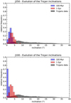 |
Fig. 6 Inclination distribution of the Jupiter Trojans at t = 100 Myr (in blue) and at t = 1 Gyr (in red). In the top histogram we plot the Trojan inclinations resulting from simulation J250. In the bottom histogram we show the Trojan inclinations resulting from simulation J100. In grey we plot the current observed inclination distribution of the Trojans. |
Evolution of the number of massless Trojans, planetary embryos, and asymmetry ratio for simulations JS250 and JS100.
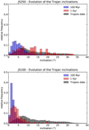 |
Fig. 7 Inclination distribution of the Jupiter Trojans at t = 100 Myr (in blue) and t = 500 Myr (in red). In the top histogram we show the Trojan inclinations resulting from simulation JS250. In the bottom histogram we plot the Trojan inclinations resulting from simulation JS100. In grey we denote the current observed inclination distribution of the Trojans. |
3.2.3 10EMBRYOS
In order to complete the study of the embryo case, we decided to perform a small statistical study about the probability of losing massive Trojans from the swarms. Because simulations with almost one hundred massive bodies are computational expensive, we decided to run ten simulations with the growth tracks of Jupiter an Saturn in which we substituted only ten of their Trojans by Ceres-like bodies in a random way, that is, we did not choose in which swarm they were located. We list the parameters of these runs in Table 5. In all the ten runs at least one massive embryo was left in one of the swarms. Even when in six runs no massive embryo survived in the L5 swarm, it is apparently very hard to deplete both swarms in the same run.
We conclude that the hypothesis of embryos embedded in the Trojan swarms presents two main problems: (a) it is hard to remove the last embryos in the swarms, and (b) the presence of embryos can heavily affect the original asymmetry ratio by decreasing it, increasing it, and also reversing it.
Planetary embryos left in each swarm in the 10EMBRYO simulations.
3.3 JPRESTIRRED and JSPRESTIRRED
In the last scenario, we tested the resulting Trojan orbital proprieties when they are captured from an already pre-stirred disc. The simulations were exactly the same as J0 and JS0. We just modified the low massless body inclinations and eccentricities in the disc.
3.3.1 JPRESTIRRED_AB and JSPRESTIRRED_AB
In the JPRESTIRRED_AB and JSPRESTIRRED_AB simulations, we kept track of the number of Trojans and their asymmetry ratio during t = 4.5 Gyr of evolution.
When only Jupiter is present in the system (JPRESTIRRED_AB), Table 6 shows that Jupiter captures a number of Trojans of the same order as the Trojans obtained in J0. The depletion of the mass is not effective over t = 4.5 Gyr, as it was in J0. The asymmetry is instead smaller than in J0 and remains similar to the initial asymmetry. The low ratio is due to less efficiency in the mechanism that generates the asymmetry in the pre-stirred case in which Jupiter alone is involved. When we experimented with letting Jupiter start at 23 and 29.5 au as well, we obtained asymmetries of about 1.3 and 1.4, respectively as shown in Fig. 8. We computed the arithmetic mean of the values found in the ten simulations for each case, and the uncertainty is represented by the unbiased standard deviation. The current asymmetry ratio is also highlighted in green. For the asymmetry ratio error, a propagation of the uncertainty is applied.
When we analyse the case where Saturn is added to the system (JSPRESTIRRED_AB), we note that the number of particles trapped as Trojans is much lower than in the JPRESTIRRED_AB simulations. Perturbations exerted by Saturn on Jupiter Trojans are probably again very effective on already pre-stirred disc particles. The final mass of the Trojans is of the order of 10−2 M⊕, which is still significantly higher than the mass of the current Trojans, which is roughly 10−5 M⊕ (Vinogradova & Chernetenko 2015), but we need to account for an additional depletion due to the late instability of the giant planets, as we discussed in Sect. 2. The asymmetry is also smaller than in the flat disc case, but it remains of the same order. At t = 4.5 Gyr only a few Trojans are left in the swarms, and fluctuations in the depletion history can heavily affect the asymmetry, therefore the last number is not particularly meaningful.
The inclination distribution of the Jupiter Trojans in simulation JPRESTIRRED_AB are shown in the top panel of Fig. 9. Aerodynamic gas drag is not effective in the outer Solar System while the Trojans are trapped. Particles spend 2 Myr in the disc before Jupiter starts to grow, but in this time span, eccentricities and inclinations are not damped enough to get a flat disc. The shape of the inclination distribution is instead preserved in the Trojan population distribution. When we analyse the results at t = 5 Myr, we note that the quasi-invariance of the inclinations of the Jupiter Trojans under mass growth and inner migration of the gas giant (Fleming & Hamilton 2000) also holds for the higher inclinations of the pre-stirred disc. The same is true when we add Saturn to the system, as shown in the bottom panel of Fig. 9: disc particles preserve the high inclination distribution in the captured Jupiter Trojan population, but the presence of Saturn also shapes it in a way that is more similar to the current inclination distribution of the Trojans.
Evolution of the number of Trojans, their mass and asymmetry ratio for simulations JPRESTIRRED_AB, JSPRESTIRRED_AB, JPRESTIRRED_CKBO and JSPRESTIRRED_CKBO.
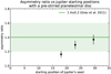 |
Fig. 8 The asymmetry ratio of the Jupiter Trojans obtained starting Jupiter’s seed in different positions: 18 au (nominal case), 23 auand 29.5 au. This is the case with simulations with only Jupiter involved and an initial planetesimal disc stirred to values resembling the asteroid belt inclination and eccentricity distributions. The current asymmetry ratio of the Jupiter Trojans is highlighted in green. |
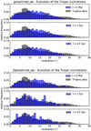 |
Fig. 9 Top panel: inclination distribution of the Jupiter Trojans at t = 5 Myr (top histogram), t = 1 Gyr (middle histogram), and t = 4.5 Gyr (bottom histogram) from simulation JPRESTIRRED_AB. Bottom panel: inclination distribution of the Jupiter Trojans at t = 5 Myr (top histogram), t = 1 Gyr (middle histogram), and t = 4.5 Gyr (bottom histogram) from simulation JSPRESTIRRED_AB. |
3.3.2 JPRESTIRRED_CKBO and JSPRESTIRRED_CKBO
In the JPRESTIRRED_CKBO and JSPRESTIRRED_CKBO simulations, we kept track of the number of trapped Trojans and their asymmetry ratio during an evolution of t = 4.5 Gyr, as in the previous cases. We report the data in Table 6. As in JPRESTIRRED_AB, the number of Trojans captured in simulation JPRESTIRRED_CKBO is of the same order as thenumber of Trojans in the flat disc case with Jupiter alone (J0); the depletion in mass is also very small and the asymmetry ratio is of the same order and follows the evolution of the simulation JPRESTIRRED_AB. The same analogies apply between simulation JSPRESTIRRED_CKBO and JSPRESTIRRED_AB: fewer particles are captured as Trojans, the swarms are significantly depleted, and the asymmetry ratio remains of the same order. The inclination distribution of JPRESTIRRED_CKBO preserves the initial shape, as happened for JPRESTIRRED_AB, as shown in the top panel of Fig. 10. When Saturn is added (JSPRESTIRRED_CKBO), the Trojans instead remain highly inclined, but the initial shape is not recognisable (Fig. 10, bottom panel), which also holds for JSPRESTIRRED_AB. For the final total mass of the Trojans in these simulations, we obtained similar results as in the JPRESTIRRED_AB and JSPRESTIRRED_AB cases.
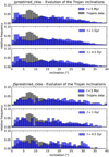 |
Fig. 10 Top panel: inclination distribution of the Jupiter Trojans at t = 5 Myr (top histogram), t = 1 Gyr (middle histogram), and t = 4.5 Gyr (bottom histogram) from simulation JPRESTIRRED_CKBO. Bottom panel: inclination distribution of the Jupiter Trojans at t = 5 Myr (top histogram), t = 1 Gyr (middle histogram), and t = 4.5 Gyr (bottom histogram) from simulation JSPRESTIRRED_CKBO. |
4 Discussions and conclusions
We tested different possibilities in order to explain the high inclination distribution observed in the Jupiter Trojans: (1) secular evolution of an initially flat Trojan population, (2) embryos embedded in the Trojan swarms, and (3) pre-stirred planetesimals trapped as Trojans. All of our simulations are based on the core accretion model boosted by pebble accretion, which allows the cores of the giant planets to grow fast enough to accrete gas from the protoplanetary disc. While the protoplanets are growing, they also experience inward migration because of interactions with the surrounding gas. The resulting scenario is a large-scale migration of a growing Jupiter until the gas of the protoplanetary disc is still available, which in our case is 3 Myr. Based on our results, our main conclusions are listed below.
- (a)
When Jupiter Trojans are captured from a disc of particles with zero inclinations, their secular evolution does not result inany significant increase of their inclinations. The inclination distribution will remain very flat during the evolution of 4.5 Gyr of the Solar System. The system is also very stable when Jupiter is alone in the system, that is, there is no depletion of the Trojans’ mass. When Saturn is added to the system, perturbations between the planets will lead to a less efficient capture (15% less), to a slight increase in inclinations of the Trojans, and to a depletion of the swarms of the order of about 40%. It is highly unlikely, however, that the planetesimal disc in which planetary embryos form would remain unaffected by the presence of massive bodies and hence remain very flat when Jupiter was growing.
- (b)
When massive planetesimals are embedded in the Trojan swarms, the inclination distribution of the Trojans can evolve toagree with the current distribution, especially if the embryos are at least of similar mass to Pluto. Moreover, embryos are very effective in depleting the swarms. It is important to note that an uneven distribution of the embryos in between the two swarms can affect the original asymmetry and can even reverse it. This means that in the massive-embryo model, the current observed asymmetry in the Jupiter Trojans might not reflect the initial asymmetry that is generated in the early inward migration and growth of the gas giant. The main problem is represented by the necessity of removing the embryos during the evolution of 4.5 Gyr of the Solar System because the current Trojan population includes no very massive asteroid. In none of our set of simulations did we successfully lose all the embryos from both the swarms. When one of the swarms is left with just one embryo, embryo–embryo scattering is no longer possible, and the probability that the massive object is lost would be that of a massless Trojan: it would just depend on its eccentricity and inclination (Levison et al. 1997).
- (c)
When we considered a pre-stirred planetesimal disc and added Saturn to the simulations, our captured Trojan population was less massive than that of the flat disc case by an order of magnitude. The subsequent depletion also accounts for another order of magnitude in the mass loss. Finally, the late instability would at least account for another substantial depletion, that is, at least 80%, as found by Pirani et al. (2019). The resulting Trojans preserve the initial high inclination distribution, which is very similar to the current distribution. The asymmetry when Jupiter alone migrates is lower than in the other cases, and this is to be attributed to a lower efficiency in generating the asymmetry. Starting Jupiter slightly farther away from the Sun generates an asymmetry consistent with the observed asymmetry.
We stress that estimating the mass of each particle, and hence the mass of the Trojan population, is based on the minimum mass solar nebula, a model that does not necessarily represent the primordial planetesimal populations because the planets migrate in the disc during their formation. Hence, any computation of the absolute value of the mass of the Trojans is to be taken with a grain of salt. Moreover, the late instability of the giant planets has not been simulated in this paper because the mechanism, time, and timescales of this event are still uncertain. A good portion of the Trojan mass is probably lost in this event, as shown by Pirani et al. (2019), who estimated that only roughly 20% of the Jupiter Trojans survive if the giant planet suddenly jumps from 5.4 to 5.2 au. We conclude that a pre-stirred planetesimal disc is the most likely scenario for the Trojans’ capture because this can simultaneously explain the high inclinations, the low total mass, and the asymmetry ratio of the Jupiter Trojans.
Acknowledgements
We would like to thank the anonymous referee for the helpful comments. SP, AJ and AM are supported by the project grant “IMPACT” from the Knut and Alice Wallenberg Foundation (grant 2014.0017). A.J. was further supported by the Knut and Alice Wallenberg Foundation grants 2012.0150 and 2014.0048, the Swedish Research Council (grant 2018-04867) and the European Research Council (ERC Consolidator Grant 724687- PLANETESYS). The computations are performed on resources provided by the Swedish Infrastructure for Computing (SNIC) at the LUNARC-Centre in Lund and partially funded by the Royal Physiographic Society of Lund through a grant.
References
- Abod, C. P., Simon, J. B., Li, R., et al. 2019, ApJ, 883, 192 [Google Scholar]
- Barucci, M. A., Cruikshank, D. P., Mottola, S., & Lazzarin, M. 2002, Physical Properties of Trojan and Centaur Asteroids, eds. W. F. Bottke, Jr., A. Cellino, P. Paolicchi, & R. P. Binzel (Tucson: University of Arizona Press), 273 [Google Scholar]
- Bitsch, B., Lambrechts, M., & Johansen, A. 2015, A&A, 582, A112 [NASA ADS] [CrossRef] [EDP Sciences] [Google Scholar]
- Bottke, W. F., Durda, D. D., Nesvorný, D., et al. 2005, Icarus, 175, 111 [NASA ADS] [CrossRef] [Google Scholar]
- Chambers, J. E. 1999, MNRAS, 304, 793 [NASA ADS] [CrossRef] [MathSciNet] [Google Scholar]
- Chambers, J. E., & Wetherill, G. W. 2001, Meteorit. Planet. Sci., 36, 381 [NASA ADS] [CrossRef] [Google Scholar]
- DeMeo, F. E.,& Carry, B. 2014, Nature, 505, 629 [NASA ADS] [CrossRef] [Google Scholar]
- Duncan, M. J., Levison, H. F., & Lee, M. H. 1998, AJ, 116, 2067 [NASA ADS] [CrossRef] [EDP Sciences] [Google Scholar]
- Fleming, H. J., & Hamilton, D. P. 2000, Icarus, 148, 479 [NASA ADS] [CrossRef] [Google Scholar]
- Gomes, R., Levison, H. F., Tsiganis, K., & Morbidelli, A. 2005, Nature, 435, 466 [NASA ADS] [CrossRef] [PubMed] [Google Scholar]
- Grav, T., Mainzer, A. K., Bauer, J., et al. 2011, ApJ, 742, 40 [NASA ADS] [CrossRef] [Google Scholar]
- Hayashi, C. 1981, Prog. Theor. Phys. Suppl., 70, 35 [NASA ADS] [CrossRef] [MathSciNet] [Google Scholar]
- Ida, S., Guillot, T., & Morbidelli, A. 2016, A&A, 591, A72 [NASA ADS] [CrossRef] [EDP Sciences] [Google Scholar]
- Johansen, A., & Lacerda, P. 2010, MNRAS, 404, 475 [NASA ADS] [Google Scholar]
- Johansen, A., & Lambrechts, M. 2017, Ann. Rev. Earth Planet. Sci., 45, 359 [NASA ADS] [CrossRef] [Google Scholar]
- Johansen, A., Blum, J., Tanaka, H., et al. 2014, in Protostars and Planets VI, eds. H. Beuther, R. S. Klessen, C. P. Dullemond, & T. Henning (Tucson: University of Arizona Press), 547 [Google Scholar]
- Kokubo, E., & Ida, S. 2000, Icarus, 143, 15 [NASA ADS] [CrossRef] [Google Scholar]
- Lambrechts, M., & Johansen, A. 2012, A&A, 544, A32 [Google Scholar]
- Levison, H. F., Shoemaker, E. M., & Shoemaker, C. S. 1997, Nature, 385, 42 [NASA ADS] [CrossRef] [Google Scholar]
- Lin, D. N. C., & Papaloizou, J. 1986, ApJ, 309, 846 [NASA ADS] [CrossRef] [Google Scholar]
- Lykawka, P. S., & Horner, J. 2010, MNRAS, 405, 1375 [NASA ADS] [Google Scholar]
- Mamajek, E. E. 2009, AIP Conf. Ser., 1158, 3 [Google Scholar]
- Marchis, F., Durech, J., Castillo-Rogez, J., et al. 2014, ApJ, 783, L37 [NASA ADS] [CrossRef] [Google Scholar]
- Marzari, F., & Scholl, H. 2000, Icarus, 146, 232 [NASA ADS] [CrossRef] [Google Scholar]
- Marzari, F., Scholl, H., Murray, C., & Lagerkvist, C. 2002, Origin and Evolution of Trojan Asteroids, eds. W. F. Bottke, Jr. A. Cellino, P. Paolicchi, & R. P. Binzel (Tucson: University of Arizona Press), 725 [Google Scholar]
- Minton, D. A., & Malhotra, R. 2010, Icarus, 207, 744 [NASA ADS] [CrossRef] [Google Scholar]
- Morbidelli, A., Levison, H. F., Tsiganis, K., & Gomes, R. 2005, Nature, 435, 462 [NASA ADS] [CrossRef] [PubMed] [Google Scholar]
- Morbidelli, A., Nesvorny, D., Laurenz, V., et al. 2018, Icarus, 305, 262 [NASA ADS] [CrossRef] [Google Scholar]
- Nesvorný, D. 2011, ApJ, 742, L22 [NASA ADS] [CrossRef] [Google Scholar]
- Nesvorný, D., Vokrouhlický, D., & Morbidelli, A. 2013, ApJ, 768, 45 [NASA ADS] [CrossRef] [Google Scholar]
- O’Brien, D. P., Morbidelli, A., & Bottke, W. F. 2007, Icarus, 191, 434 [NASA ADS] [CrossRef] [MathSciNet] [Google Scholar]
- Ormel, C. W., & Klahr, H. H. 2010, A&A, 520, A43 [NASA ADS] [CrossRef] [EDP Sciences] [Google Scholar]
- Petit, J.-M., Morbidelli, A., & Valsecchi, G. 1998, BAAS, 30, 1453 [NASA ADS] [Google Scholar]
- Petit, J.-M., Morbidelli, A., & Chambers, J. 2001, Icarus, 153, 338 [NASA ADS] [CrossRef] [Google Scholar]
- Pirani, S., Johansen, A., Bitsch, B., Mustill, A. J., & Turrini, D. 2019, A&A, 623, A169 [NASA ADS] [CrossRef] [EDP Sciences] [Google Scholar]
- Pollack, J. B., Hubickyj, O., Bodenheimer, P., et al. 1996, Icarus, 124, 62 [NASA ADS] [CrossRef] [Google Scholar]
- Schäfer, U., Yang, C.-C., & Johansen, A. 2017, A&A, 597, A69 [NASA ADS] [CrossRef] [EDP Sciences] [Google Scholar]
- Tsiganis, K., Gomes, R., Morbidelli, A., & Levison, H. F. 2005, Nature, 435, 459 [NASA ADS] [CrossRef] [PubMed] [Google Scholar]
- Vinogradova, T. A., & Chernetenko, Y. A. 2015, Sol. Syst. Res., 49, 391 [NASA ADS] [CrossRef] [Google Scholar]
- Volk, K., & Malhotra, R. 2011, ApJ, 736, 11 [NASA ADS] [CrossRef] [Google Scholar]
- Walsh, K. J., Morbidelli, A., Raymond, S. N., O’Brien, D. P., & Mandell, A. M. 2011, Nature, 475, 206 [NASA ADS] [CrossRef] [PubMed] [Google Scholar]
- Ward, W. R. 1997, Icarus, 126, 261 [NASA ADS] [CrossRef] [Google Scholar]
- Weidenschilling, S. J. 1977, MNRAS, 180, 57 [NASA ADS] [CrossRef] [Google Scholar]
- Wetherill, G. W. 1992, Icarus, 100, 307 [NASA ADS] [CrossRef] [Google Scholar]
- Williams, J. P., & Cieza, L. A. 2011, ARA&A, 49, 67 [NASA ADS] [CrossRef] [Google Scholar]
- Wisdom, J., & Holman, M. 1991, AJ, 102, 1528 [NASA ADS] [CrossRef] [Google Scholar]
All Tables
Evolution of the number of Trojans, their total mass, and the asymmetry ratio for simulations J0 and JS0.
Evolution of the number of massless Trojans, planetary embryos, and asymmetry ratio for simulations J250 and J100.
Evolution of the number of massless Trojans, planetary embryos, and asymmetry ratio for simulations JS250 and JS100.
Evolution of the number of Trojans, their mass and asymmetry ratio for simulations JPRESTIRRED_AB, JSPRESTIRRED_AB, JPRESTIRRED_CKBO and JSPRESTIRRED_CKBO.
All Figures
|
Fig. 1 Growth tracks of Jupiter and Saturn. The gas giants start with an initial mass of 10−2 M⊕ and grow to their current mass. Jupiter migrates from 18 au to its current orbit at 5.2 au and Saturn migrates from 21 au to 9.5 au. The migration starts at ~2.2 Myr and stops when the gas dissipates at 3 Myr. The green solid line corresponds to the core accretion phase, the orange solid line corresponds to the gas accretion phase, and the cyan solid line corresponds to the runaway gas accretion phase. |
| In the text | |
|
Fig. 2 Starting inclinations for J0 (blue histogram) and JS0 (red histogram) at 5 Myr. The grey histogram represents the current inclination distribution of Jupiter Trojans. |
| In the text | |
|
Fig. 3 Size frequency distributions of the Jupiter Trojans in the case of Rmin = 100 km and Rexp = 250 km (top histogram) and for Rmin = 10 km and Rexp = 100 km (bottom histogram). The histograms show the number of Trojans in mass bins (bottom x-axis). In the upper x-axes we show the correspondent radius bins (we assumed a density of the Trojans of 1.5 g cm−3). In cyan we highlight the part of the distributions that we substituted into the Trojan swarms as massive bodies. The black arrow indicates the mass of asteroid (624) Hektor, which is the most massive Jupiter Trojan. |
| In the text | |
|
Fig. 4 In the JPRESTIRRED_AB and JSPRESTIRRED_AB simulations we used an inclination distribution model similar to the asteroid belt distribution (top histogram). In the JPRESTIRRED_CKBO and JSPRESTIRRED_CKBO simulations we used an inclination distribution model similar to the CKBOs distribution (bottom histogram). |
| In the text | |
|
Fig. 5 Inclination distribution of the Jupiter Trojans at t = 4.5 Gyr for the case of Jupiter migrating alone (J0) in blue and for the case of Jupiter and Saturn both migrating (JS0) in red. In thesesimulations all the Trojans are massless. In grey we plot the current observed inclination distribution of the Trojans. |
| In the text | |
|
Fig. 6 Inclination distribution of the Jupiter Trojans at t = 100 Myr (in blue) and at t = 1 Gyr (in red). In the top histogram we plot the Trojan inclinations resulting from simulation J250. In the bottom histogram we show the Trojan inclinations resulting from simulation J100. In grey we plot the current observed inclination distribution of the Trojans. |
| In the text | |
|
Fig. 7 Inclination distribution of the Jupiter Trojans at t = 100 Myr (in blue) and t = 500 Myr (in red). In the top histogram we show the Trojan inclinations resulting from simulation JS250. In the bottom histogram we plot the Trojan inclinations resulting from simulation JS100. In grey we denote the current observed inclination distribution of the Trojans. |
| In the text | |
|
Fig. 8 The asymmetry ratio of the Jupiter Trojans obtained starting Jupiter’s seed in different positions: 18 au (nominal case), 23 auand 29.5 au. This is the case with simulations with only Jupiter involved and an initial planetesimal disc stirred to values resembling the asteroid belt inclination and eccentricity distributions. The current asymmetry ratio of the Jupiter Trojans is highlighted in green. |
| In the text | |
|
Fig. 9 Top panel: inclination distribution of the Jupiter Trojans at t = 5 Myr (top histogram), t = 1 Gyr (middle histogram), and t = 4.5 Gyr (bottom histogram) from simulation JPRESTIRRED_AB. Bottom panel: inclination distribution of the Jupiter Trojans at t = 5 Myr (top histogram), t = 1 Gyr (middle histogram), and t = 4.5 Gyr (bottom histogram) from simulation JSPRESTIRRED_AB. |
| In the text | |
|
Fig. 10 Top panel: inclination distribution of the Jupiter Trojans at t = 5 Myr (top histogram), t = 1 Gyr (middle histogram), and t = 4.5 Gyr (bottom histogram) from simulation JPRESTIRRED_CKBO. Bottom panel: inclination distribution of the Jupiter Trojans at t = 5 Myr (top histogram), t = 1 Gyr (middle histogram), and t = 4.5 Gyr (bottom histogram) from simulation JSPRESTIRRED_CKBO. |
| In the text | |
Current usage metrics show cumulative count of Article Views (full-text article views including HTML views, PDF and ePub downloads, according to the available data) and Abstracts Views on Vision4Press platform.
Data correspond to usage on the plateform after 2015. The current usage metrics is available 48-96 hours after online publication and is updated daily on week days.
Initial download of the metrics may take a while.