| Issue |
A&A
Volume 674, June 2023
|
|
|---|---|---|
| Article Number | A138 | |
| Number of page(s) | 12 | |
| Section | Celestial mechanics and astrometry | |
| DOI | https://doi.org/10.1051/0004-6361/202346223 | |
| Published online | 16 June 2023 | |
The invasion of a free-floating planet and the number asymmetry of Jupiter Trojans
1
School of Astronomy and Space Science, Nanjing University,
163 Xianlin Avenue,
Nanjing
210023,
PR China
e-mail: This email address is being protected from spambots. You need JavaScript enabled to view it.
2
Key Laboratory of Modern Astronomy and Astrophysics in Ministry of Education, Nanjing University,
Nanjing
210023,
PR China
3
Department of Mathematics, Northwestern University,
2033 Sheridan Road,
Evanston, IL
60208,
USA
4
New York University Abu Dhabi,
PO Box 129188
Abu Dhabi,
United Arab Emirates
5
Center for Astro, Particle and Planetary Physics (CAP3), New York University Abu Dhabi,
PO Box 129188
Abu Dhabi,
United Arab Emirates
6
University of Occupational and Environmental Health,
1-1 Iseigaoka,
Yahata, Kitakyusyu
807-8555,
Japan
7
Planetary Exploration Research Center, Chiba Institute of Technology,
2-17-1 Tsudanuma,
Narashino, Chiba
275-0016,
Japan
Received:
23
February
2023
Accepted:
25
April
2023
Abstract
Context. This paper extends our previous study of the early evolution of Jupiter and its two Trojan swarms by introducing the possible perturbations of a free-floating planet (FFP) invading the Solar System.
Aims. In the framework of the invasion of a FFP, we aim to provide some new scenarios to explain the number asymmetry of the L4 and L5 Jupiter Trojans, as well as some other observed features (e.g. the resonant amplitude distribution).
Methods. We investigate two different cases: (i) the indirect case, where Jupiter experiences a scattering encounter with the FFP and jumps outwards at a speed that is sufficiently high to make the L4 point temporarily disappear, resulting in a change in the numbers of the L4 (N4) and L5 (N5) Trojan swarms; (ii) the direct case, in which the FFP traverses the L5 region and affects the stability of the local Trojans.
Results. In the indirect case, the outward migration of Jupiter can be fast enough to make the L4 islands disappear temporarily, inducing an increase in the resonant amplitude of local Trojans. After the migration is over, the L4 Trojans come back to the reappeared and enlarged islands. As for the L5 islands, they always exist but expand even more considerably. Since the L4 swarm suffers less excitation in the resonant amplitude than the L5 swarm, more L4 Trojans are stable and could survive to the end. In the direct case, the FFP could deplete a considerable fraction of the L5 Trojans, while the L4 Trojans at large distances are not affected and all of them could survive.
Conclusions. Both the indirect and direct cases could result in a number ratio of R45 = N4/N5 ~ 1.6 that can potentially explain the current observations. The latter has the advantage of producing the observed resonant amplitude distribution. To achieve these results, we propose that the FFP should have a mass of at least of a few tens of Earth masses and its orbital inclination should be allowed to be as high as 40°.
Key words: methods: miscellaneous / minor planets, asteroids: general / planets and satellites: individual: Jupiter / planets and satellites: dynamical evolution and stability / celestial mechanics
© The Authors 2023
 Open Access article, published by EDP Sciences, under the terms of the Creative Commons Attribution License (https://creativecommons.org/licenses/by/4.0), which permits unrestricted use, distribution, and reproduction in any medium, provided the original work is properly cited.
This article is published in open access under the Subscribe to Open model. This email address is being protected from spambots. You need JavaScript enabled to view it. to support open access publication.
1 Introduction
In 1772, J. L. Lagrange showed that there are two equilibrium points in the orbital plane of two massive bodies around which small mass bodies can remain. Later in 1906, Max Wolf at the Heidelberg Observatory discovered an asteroid (588 Achilles) at a distance from the Sun similar to that of Jupiter (Nicholson 1961). Since then, more and more asteroids that share the orbit of Jupiter have been discovered. As Lagrange’s theory predicted, there are two swarms of these asteroids, leading or trailing Jupiter by about 60° in longitude, that is, around the L4 or L5 triangular Lagrangian point. The asteroids ahead of Jupiter are called the L4 Jupiter Trojans, while the others behind Jupiter are the L5 Jupiter Trojans.
For decades, it has been known that there are many more objects in the L4 swarm than in the L5 one (Shoemaker et al. 1989; Jewitt et al. 2004; Freistetter 2006; Nakamura & Yoshida 2008; Grav et al. 2011, 2012; Slyusarev 2013; Li & Sun 2018). This number discrepancy still holds today, even when more than 11000 Jupiter Trojans have been discovered. The unbiased leading-to-trailing number ratio is estimated to be about 1.6 (Szabó et al. 2007). In the current configuration of the Solar System, the L4 and L5 Trojan swarms show a comparable dynamical stability and survivability properties (Di Sisto et al. 2014, Di Sisto et al. 2019; Holt et al. 2020). Thus, the significant number difference should arise at earlier times of our Solar System’s life, and it remains a profound mystery in the evolutionary history of Jupiter Trojans.
In a very recent work (Li et al. 2023), we have developed a new mechanism that may explain the number asymmetry of Jupiter Trojans. We propose that an outward migration of Jupiter, caused by the giant planet instability in the early Solar System, can induce different evolutional paths for the two Trojan swarms. In this dynamical model, the L4 Trojans can have their resonant amplitudes decreased due to the contraction of the L4 region and they would become more stable. Oppositely, the L5 Trojans’ resonant amplitudes increase because of the expansion of the L5 region and therefore they would become more unstable. As a result, there are more surviving Trojans in the L4 swarm than in the L5 one. As long as the outward migration of Jupiter is fast enough, at a speed of  AUyr−1 (
 denotes the variation of Jupiter’s semi-major axis aJ), this mechanism could provide a natural explanation for the unbiased observation that the L4 Trojans are about 1.6 times more than the asteroids in the L5 swarm.
The fast outward migration of Jupiter can always be capable of inducing a leading-to-trailing number ratio of R45 > 1, and theoretically speaking, the resulting L4–L5 asymmetry should be even more significant as long as the migration of Jupiter is faster. Regarding this rapid migration of Jupiter, in Li et al. (2023), we consider the mechanism of early dynamical instability among the giant planets in the outer Solar System (see Nesvorný 2018 for a review). When Jupiter experienced a close encounter with the fifth outer planet, which left the Solar System eventually, it could migrate outwards at a speed of about 1.5 × 10⁻⁴ AUyr−1 (Nesvorný et al. 2013), as we mentioned above. For this dynamical model confined within the Solar System, the migration speed of Jupiter is limited. Thus, in order to achieve the number asymmetry of R45 ~ 1.6, we have to assume that the Trojans initially possess moderately large resonant amplitudes of ≥30º.
In this paper, we extend the previous work by considering a much faster migration of Jupiter, which could be produced by the invasion of a free-floating planet (FFP). Observations have shown that the number of FFPs with Jupiter mass can exceed that of main sequence stars in our Galaxy (Sumi et al. 2011). Although the probability of capturing a FFP is only a few per cent or even lower in planetary systems (Li & Adams 2016; Parker et al. 2017; Goulinski & Ribak 2018), a penetrating flyby in the Solar System could be more likely. If a FFP happened to interact with Jupiter, depending on the minimum mutual distance, Jupiter could migrate outwards by a considerable distance. Since the timescale of this process is very short and nearly fixed for various FFPs with perihelia around the orbit of Jupiter, as we subsequently show in Sect. 2, the migration speed of Jupiter can be quite high.
According to Sicardy & Dubois (2003), there is a critical migration speed of  AU yr−1. The jumping-Jupiter models constructed in Li et al. (2023) exclusively consider the speed values of
  below this limit, indicating the persistent existence of the L4 islands and thus the possible survival of the local Trojans. But, due to the gravitational acceleration of the FFP, Jupiter could jump outwards at a speed of
  , leading to the disappearance of the L4 islands. Thus, it is of great interest to understand how the L4 Trojans would be influenced.
Besides the fast outward migration of Jupiter caused by the FFP, a second potential mechanism of producing the number asymmetry of Jupiter Trojans in the case that a FFP once invaded the L5 region is also explored. Actually, Nesvorný et al. (2013) proposed that after Jupiter Trojans are captured, an extra ice giant can still remain on the Jupiter-crossing orbit. If this ice giant occasionally traverses the L5 region, a fraction of the local Trojans would be scattered away. Since the other group of Trojans in the L4 region are far away from this ice giant, their stability is not affected. Obviously, a L4-to-L5 number ratio of R45 > 1 would appear. The authors found that in one case, R45 can reach a value of about 1.3, which seems not large enough to explain the current asymmetry of R45 ~ 1.6. Possibly, the number asymmetry generated in this scenario could be more significant if the perturbations on the L5 Trojans are stronger, for instance, by increasing the mass of the invading planet. However, in the model of Nesvorný et al. (2013), the planet invading the L5 region cannot have sufficiently large mass because it is an ice giant and should have a mass comparable to that of Uranus/Neptune. But if we consider the invading planet to be a FFP, it could be much more massive, up to the order of Jupiter mass.
In this paper, as a follow-up work of our study of the number asymmetry of Jupiter Trojans, we investigate the influence of a FFP invading the Solar system. The rest of this paper is organised as follows: in Sect. 2, we investigate the outward migration of Jupiter at a very high speed due to the close encounter with the FFP, and the concomitant evolution of Jupiter Trojans that may explain the unbiased L4-to-L5 number ratio of R45 ~ 1.6. In Sect. 3, we investigate another potential mechanism of producing the number asymmetry of Jupiter Trojans in the case that the FFP once penetrated the L5 region and dispersed a large fraction of the local population. In Sect. 4, we summarise the results and provide some discussions.
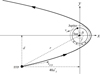 |
Fig. 1 Schematic diagram of the jumping-Jupiter evolution due to the invasion of a FFP in the co-planar model. Jupiter is initially on a circular orbit (solid circle) around the Sun, with phase angle θ measured anticlockwise from the positive x-axis. The FFP is approaching the Sun-Jupiter system on a parabolic orbit with initial coordinates ( |

2 Indirect case: Jupiter jumping caused by a FFP
As we described in the introduction, a FFP could visit the Solar System on an unbound orbit and possibly pass close to Jupiter. During the time of such close encounter, the FFP could accelerate Jupiter’s motion, inducing the increase of Jupiter’s semi-major axis by an amplitude of ΔaJ. Due to the short period of the FFP’s strong perturbation, the migration timescale Δt of Jupiter should equivalently be very small. Therefore, the migration rate of Jupiter, that is  , could be much higher than that considered in Li et al. (2023). Obviously, the reasonable values of ΔaJ and At are to be determined by the orbit of the FFP.
2.1 Orbit of the FFP
In order to investigate the FFP’s gravitational effect on Jupiter’s migration, we simply use a three-body system consisting of the Sun with mass M⊙, Jupiter with mass mJ and an incoming FFP with mass mFFP (see Fig. 1). The Sun is fixed at the origin of the coordinate system (x, y). In this heliocentric framework, Jupiter initially moves on a Keplerian circular orbit; and similar to Varvoglis et al. (2012), the FFP is introduced to start on a parabolic trajectory. We assume that the orbits of these three bodies are all in the same plane.
If we consider Jupiter to be moving anticlockwise around the Sun on a circular orbit, then, the initial positions and velocities of Jupiter can be expressed as
 (1)
(1)
where  denotes the semi-major axis of the unperturbed orbit of Jupiter and is taken to be 5.2 AU, θ is Jupiter’s initial position angle (anticlockwise from the positive x-axis), and the initial linear velocity can be calculated by
 (2)
(2)
Here, and throughout the following, the bracketed digit 0 indicates the initial value of each parameter at the time t = 0.
The FFP is initially started at ( , −d) (d > 0), having a parabolic velocity of υFFP with respect to the Sun. Then the parameter d controls the FFP’s perihelion, which will be kept outside the orbit of Jupiter to avoid the collision event as we illustrate below. The orbit of the FFP can be described by
 (3)
(3)
where r is the radial distance, f is the true anomaly, and p is the semilatus rectum that can be determined by the initial coordinates. Then the initial conditions of the FFP can be written as
 (4)
(4)
where  .
.
For the system’s initial conditions described above by Eqs. (1) and (4), there are three free parameters: θ for Jupiter, d and mFFP for the FFP. The initial phase angle θ determines the location of Jupiter when the FFP is close to Jupiter’s orbit. The initial y-distance d determines where exactly the FFP’s perihelion (p/2, 0) is, and accordingly the minimum distance between the FFP and Jupiter. Finally, the mass mFFP determines the strength of the FFP’s perturbation from a certain distance. Therefore, the gravitational effect of the FFP on Jupiter could be very sensitive to these three parameters.
First, in order to avoid a collision between Jupiter and the FFP, we need to adopt the value of d satisfying the condition p / 2 >  . Let r(0) be the initial radial distance of the FFP, we have
 (5)
(5)
where
 (6)
(6)
Substituting for x(0) and y(0) from Eq. (4) into Eqs. (5) and (6), we get
 (7)
(7)
This condition can guarantee that the FFP will always be outside the orbit of Jupiter and supply the perturbing acceleration for Jupiter’s migration via a close encounter, as visualised in Fig. 1.
Second, in order for a close encounter to be achieved, it is required that the FFP comes close to the actual position of Jupiter and not only to its orbit. Having this in mind, we would design the configuration in a way that both of the FFP and Jupiter could cross the positive x-axis upwards at the same time, denoted by t*. At this epoch, the FFP is located at its perihelion with f= 0. Utilising the angular momentum integral of the two-body system comprising the Sun and the FFP
 (8)
(8)
and the transformation of Eq. (3), we can obtain
 (9)
(9)
Integrating both sides of Eq. (9) yields
 (10)
(10)
where n is the FFP’s mean motion given by
 (11)
(11)
and the integral constant t* is the time of perihelion passage for the FFP as we defined above. By taking the initial true anomaly f(0) of the FFP, we can eventually get
![Mathematical equation: ${t^*} = \left[ {{1 \over 2}\tan {{f\left( 0 \right)} \over 2} + {1 \over 6}{{\tan }^3}{{f\left( 0 \right)} \over 2}} \right]/\left( { - n} \right).$](/articles/aa/full_html/2023/06/aa46223-23/aa46223-23-eq23.png) (12)
(12)
Requiring that Jupiter should also reach the position ( , 0) at this very moment of t = t*, we can reversely calculate the initial position angle of Jupiter to be
 (13)
(13)
where TJ ≈ 11.86 yr is the orbital period of Jupiter with  .
.
It should be noted that, the FFP has its orbit precessing when it comes close to Jupiter due to the mutual interaction, thus the position and time of perihelion passage are actually different from (p/2, 0) and t*, respectively, but just by very small amounts. So the analytical estimation made above for the time t ≤ t* is still applicable and will be used to provide initial conditions of these two planets in what follows.
2.2 Results for jumping Jupiter
As we illustrated above, there are three free parameters to be considered: the distance d measuring the initial y-coordinate of the FFP, the mass mFFP of the FFP, and the initial position angle θ of Jupiter. After some tests, we have adopted  and mFFP = mJ for an invading FFP. Then Eq. (5) gives
  , indicating that this FFP has a perihelion at (p/2, 0) = (
 , 0). Thus, it will be exterior to the orbit of Jupiter and exerts the perturbing acceleration on Jupiter’s motion via a close encounter, as visualised in Fig. 1.
Since the orbit of the FFP is established, θ determines the minimum distance between the FFP and Jupiter, which is equivalent to the strength of their close encounter. In order to investigate the resulting jump of Jupiter, we have performed a series of numerical experiments for different values of θ. It is quite obvious that the FFP only spends a small amount of time passing through the perihelion because of its high velocity. For instance, if we pick a fraction of the FFP’s parabolic orbit where the radial distance is  , the corresponding times-pan is about 7 yr, as predicted by Eqs. (3) and (10). Therefore, in this subsection, in order to accurately simulate the behaviour of Jupiter during FFP’s pass-by, we employ the 7–8th-order Runge-Kutta-Fehlberg (RKF) algorithm with an adaptive stepsize and with a local truncation error of less than 10−15. The integration time is set to be 1000 yr, which is long enough compared to the time of the close encounter (i.e. only of the order of a few years as we just estimated).
Figure 2a shows the typical temporal evolution of Jupiter’s semi-major axis due to the brief visit of the FFP for θ = θ* = 249° as derived from Eq. (13). At the very beginning, Jupiter remains on its original orbit because the FFP is set to be coming from a distance as large as tens of  . Then, the FFP gradually approaches the orbit of Jupiter and Jupiter experiences a short period of outward migration on a timescale of about 10 yr (i.e. from ~246 yr to ~256 yr), as aJ increases by about 0.07 AU. This timing of the close encounter is well consistent with the value t* = 251 yr calculated from Eq. (12). After that, the FFP leaves the Solar System, and Jupiter switches to an expanded orbit, as indicated by the dashed circle in Fig. 1. Here, the FFP does not notably excite Jupiter’s eccentricity eJ, which is as small as about <0.01 at the end of the 1000 yr integration.
Considering the fact that, due to the interaction between the two planets, the configuration of their close encounter would be somewhat different from what we designed theoretically. In other words, the strongest acceleration for Jupiter could take place at θ-value other than θ*. Keeping the other initial conditions of the system unchanged, we repeat the 1000 yr numerical integrations by choosing θ to have a series of different values but close to θ*. The resultant migration amplitudes ΔaJ are plotted in Fig. 2b. The main feature is that within the adopted range of θ, Jupiter could experience an even larger-scale migration with ΔaJ over 0.6 AU, while the migration timescale is still at the level of ~10 yr. This way, the migration speed of Jupiter is nearly proportional to ΔaJ.
Nevertheless, there are two possible limitations on the maximum value of ΔaJ: (1) the eccentricity eJ of Jupiter would be excited to a higher value along with the increase of ΔaJ when the FFP’s perturbation becomes stronger. As shown in Fig. 2b, if we require the final eJ to be below the currently observed value of ~0.05, ΔaJ should not exceed 0.33 AU. (2) Murray-Clay & Chiang (2005) found that if Neptune migrates on a very short timescale, its asymmetric 2:1 resonance becomes unable to capture planetesimals at all. Similarly, if Jupiter migrates fast enough, its 1:1 resonance could not maintain the Trojans and all of them would escape. Therefore, a very large ΔaJ needs to be excluded, as we show below.
By now, the perihelion of the FFP is fixed since the free parameter d is adopted to be  . Of course, a more distant encounter between the FFP and Jupiter is very likely when the FFP’s perihelion increases. Bearing in mind that there is another free parameter, mFFP, and a more massive FFP could be introduced to counterbalance the weaker perturbation due to a larger relative distance for the encounter with Jupiter. Consequently, the acceleration for Jupiter’s motion, measured by ΔaJ, could still be comparable. A few additional tests with d increasing together with mFFP have been carried out. We find that the ΔaJ-profile always remains very similar with respect to that shown in Fig. 2b, while the θ-range would slightly change since the timing of the FFP’s perihelion passage is a little different. Taking the case of
  and mFFP = 10mJ for example, the perihelion of the FFP has been raised by about 2 AU, while the resulting ΔaJ can also reach quite a large value, up to 0.24 AU under the constraint of eJ ≲ 0.05.
Apart from the migration amplitude ΔaJ, we also monitor the migration timescale, which is always at the level of 10 yr. It is easy to understand that by looking at the velocities of the FFP at perihelion (i.e. f = 0):
 (14)
(14)
where we substitute for p from Eq. (5), and the subscript ‘peri’ represents the abbreviation for ‘perihelion’. The FFP’s mass mFFP has little effect on the velocity ẏperi since the Sun’s mass M⊙ is significantly larger. Besides, when d increases from  to
to  , the variation of ẏperi is only of the order of 10%. Therefore, the time span of the perihelion traversing of the FFP would only change a little, as well as the duration of the close encounter between the FFP and Jupiter.
In summary, the invasion of a FFP could force Jupiter to jump outwards with a speed of  , where ΔaJ can be as large as about 0.3 AU. Bearing in mind that, when
  exceeds the value of
  AU yr−1, in theory, the tadpole orbits around Jupiter’s L4 point would disappear (Sicardy & Dubois 2003; Ogilvie & Lubow 2006). Thus, it is very interesting to see what would happen if Jupiter’s migration speed exceeds that critical value, corresponding to ΔaJ > 0. 038 AU for the 10 yr migration timescale found here. This is the fundamental difference between this work and Li et al. (2023).
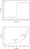 |
Fig. 2 Invading FFP with a distance parameter |

2.3 Results for L4-L5 asymmetry
In this subsection, we study the evolution of the L4 and L5 Trojans for their number asymmetry in the jumping-Jupiter model. Same as in Li et al. (2023), the radial variation of Jupiter is mimicked by using the classical formula (Malhotra 1995):
![Mathematical equation: ${a_{\rm{J}}}\left( t \right) = a_{\rm{J}}^* + {\rm{\Delta }}{a_{\rm{J}}}\left[ {1 - \exp \left( { - t/\tau } \right)} \right],$](/articles/aa/full_html/2023/06/aa46223-23/aa46223-23-eq41.png) (15)
(15)
where the e-folding time τ can represent the migration time Δt according to the correlation
 (16)
(16)
As for the test Trojans, they initially have semi-major axes  AU, eccentricities e = 0-0.3, inclinations i = 0.01, while their longitude of ascending node Ω and argument of perihelion ω are chosen randomly between 0° and 360°. Finally, the mean anomaly M is determined from the resonant angle
 (17)
(17)
where λJ is the mean longitude of Jupiter. For clarity, we denote the initial resonant angle as σ0. For the L4 and L5 swarms, we set σ0 to be 60° + Δσ0 and −60° − Δσ0, respectively, it means that these two populations are initially displaced from individual Lagrangian points by Δσ0. The number Nc of test Trojans for each swarm is adopted to be 500. More details can be found in Sect. 3.1 in Li et al. (2023).
Regarding the system evolution, we consider three key parameters: the amplitude ΔaJ and the e-folding time τ for Jupiter’s migration, together with the initial displacement Δσ0 of the test Trojans from the associated Lagrangian point. According to the obtained jumping-Jupiter model induced by the FFP encounter, the timescale of 10 yr gives τ = 3 yr (see Eq. (16)) and ΔaJ is allowed to vary in the range (0, 0.3] AU. For the test Trojans, we first choose samples having the standard Δσ0 of 30°− 80° as we did in Li et al. (2023), and there are 500 objects in each of the L4 and L5 swarms. Then we compute the orbital evolution of test Trojans by involving the jumping Jupiter with different ΔaJ. To fulfil a long-term simulation, we employ the swift_rmvs3 symplectic integrator developed by Levison & Duncan (1994), with a time-step of 0.05 yr. At the end of the 1 Myr integration, the numbers of surviving L4 (N4) and L5 (N5) Trojans, the corresponding number ratio of R45 = N4 /N5, and their final resonant amplitudes A4 and A5 are reported in Table 1.
We find that the L4-to-L5 number ratio R45 increases very fast with ΔaJ (equivalent to the migration speed). When ΔaJ ≥ 0.12 AU, the resulting values of R45 can be larger than 1.6, which is capable of explaining the current observations. More interestingly, at ΔaJ = 0.19 AU, R45 finally becomes infinite since some L4 Trojans can remain stable, but all the L5 ones have escaped, that is, N4 > 0 but N5 = 0. Thus, R45 could be as large as possible in the scenario of the FFP invasion. This is the major difference with Li et al. (2023). Besides, a further comparison with the results in Li et al. (2023) raises two more differences: (i) when the migration of Jupiter is faster, the number N4 of surviving L4 Trojans decreases; (ii) all the L4 Trojans have final resonant amplitudes larger than the original values deduced from the case of a non-migrating Jupiter. Both are in contrast with what we found in our previous work. As a matter of fact, since the jumping Jupiter considered here having ΔaJ = 0.12–0.19 AU and Δt = 10 yr, we immediately notice that its migration speed is beyond the critical value  corresponding to the disappearance of the L4 librational islands. All these make such a super fast migration model quite intriguing, thus it would be interesting to see the peculiar evolution path that the L4 Trojans follow.
Figure 3 sketches the tadpole orbits of the simulated Trojans in a frame rotating with the mean motion of Jupiter, before (black curves) and after (green curves) Jupiter’s jump. The orange arrows indicate the directions of all the librational motions, for both the black and green orbits. A L4 Trojan has a starting position at point A. If there is no migration of Jupiter, this object would move along the black orbit towards L4 since it initially has the maximum σ deviation. So the resonant angle σ has to decrease at the beginning of the evolution. But if Jupiter migrates outwards at a speed higher than  as we consider here, L4 will merge with L3 and the surrounding islands will disappear. As a result, the original L4 Trojans could temporarily switch to the horseshoe orbits and move towards the location of L3 (Ogilvie & Lubow 2006). As illustrate in Fig. 3, such L4 Trojan, starting from point A, first goes to point B and its resonant angle σ increases accordingly. Because the duration of this period is very short, equivalent to the 10 yr migration timescale of Jupiter, the angular distance between A and B would not be very large, that is, the increase of σ should be a limited value. When the migration of Jupiter has ceased, shortly after, the L4 libration islands will reappear and this Trojan located at point B finally settles on the green tadpole orbit which possesses a larger resonant amplitude than that of the original black one.
Corresponding to the schematic picture of Fig. 3, we present in Fig. 4 the tadpole orbits generated by direct numerical simulations for different evolutional scenarios of Jupiter. The black curve refers to the case in which no migration is imposed on Jupiter and the green curve refers to the jumping-Jupiter model by assuming ΔaJ = 0.15 AU (i.e.  AUyr−1 >
  ). Panel a shows the temporal variations of σ for the same L4 Trojan starting with Δσ0 = 30°. If there is no migration, the resonant angle σ decreases immediately at the beginning of the integration. But in the migration case, σ initially increases as this Trojan first moves towards the L3 point. At time of about 40 yr, that is, well after the 10 yr period of Jupiter’s migration, σ stops increasing because the Trojan is again restricted to the new L4 tadpole island with larger size (see the green orbit in Fig. 3). As a result, the resonant amplitude is increased, from 25° to 35°, as measured from the black and green orbits in Fig. 4a. This explains that, as presented in Table 1, the minimum A4 is about 35° for the case of ΔaJ = 0.15. Similarly, the L4 Trojans with Δσ0 > 30° will also experience the A4 enlargement and some of them may not survive eventually.
As Jupiter’s migration rate  increases, the Trojans around L4 could drift towards L3 more quickly during the temporary absence of the L4 islands. This implies that, in Fig. 3, the distance between points A and B becomes larger, leading to a much wider (green) tadpole orbit. Since the migration timescale of Jupiter is fixed, the migration speed is proportional to ΔaJ. Therefore, as ΔaJ increases, the two trends in N4 and A4 (see Table 1) can be understood from the following: (i) the effect of the jumping-Jupiter on the resonant amplitude enlargement for the L4 swarm is enhanced and all the local Trojans will change to the tadpole orbits with larger and larger A4. (ii) More and more L4 Trojans would be ejected as a result of orbital instability caused by increased A4 and thus the number N4 of survivals becomes smaller. It is important to emphasise that, even when the L4 point disappears during the short period of Jupiter’s jump, the local Trojans are still restricted on the co-orbital horseshoe orbits (Ogilvie & Lubow 2006). As we found in the numerical simulations, the surviving L4 Trojans actually have their semi-major axes increased from initial values of
  to final values of
  , together with the same change of Jupiter’s semi-major axis.
In the framework of Jupiter’s outward migration induced by the FFP encounter, the migration rate could exceed  . In this scenario, although the L4 swarm follows a totally different evolutionary path in comparison with what we observed previously in Li et al. (2023), the L5 swarm follows a similar one because the L5 Lagrangian point always persists and consequently the surrounding islands do not cease to exist. Nevertheless, since the migration rate of Jupiter is very high now, the L5 islands would expand considerably in width, as visualised by the black (original) and green (final) tadpole orbits around L5 point in Fig. 3. This leads to quite large resonant amplitudes (A5) of the surviving L5 Trojans (see Fig. 4b).
Although both the L4 and L5 Trojan populations have their resonant amplitudes increased and the instability could occur subsequently, the former has more survivors persistently. Thus, the resulting number ratio R45 is always larger than 1. This is because of the fact that, given the same migration rate  , the enlargement of the resonant amplitude is more effective for the L5 swarm than for the L4 one. As an example shown in Fig. 4, a L4 and a L5 Trojans are chosen to start with the same initial angular distances of Δσ0 = 30° from the respective Lagrangian points. If Jupiter does not migrate, they can evolve on exactly symmetric tadpole orbits (black curves) with the same resonant amplitudes. But due to the migration of Jupiter at a speed of 0.015 AUyr−1 (>
  AUyr−1), these two Trojans would change to wider tadpole orbits indicated by the green curves. We can see that both the L4 and L5 Trojans have their resonant amplitudes increased, from 25°, to 40° and 45°, respectively. Accordingly, the resonant amplitude A4 is 5° smaller than A5.
Before further proceeding, in relation to the determination of the reported number ratio R45, we would like to provide justifications for our choices of: (1) the number Nc = 500 of test Trojans for each swarm, and (2) the 1 Myr integration time. To investigate the effect of the number Nc of test Trojans on R45, for the case of ΔaJ = 0.12 in Table 1 (highlighted in bold), we performed 5 additional runs with the same parameters but distinct initial resonant angles σ0 associated to the standard Δσ0. As shown by the black curve in Fig. 5, when the number Nc of test Trojans is increased from 500 to 3000 in increments of 500, the resulting R45 values remain nearly constant in the narrow range of 1.65–1.7. This result indicates that, Nc = 500 is sufficiently large to provide reliable statistics for the number asymmetry of surviving test Trojans. Next, we investigated the time dependence of the reported number asymmetry R45, again for the case of ΔaJ = 0.12 in Table 1. To do this, we extended the integration time to 1 Gyr, which is of the same order of magnitude as the age of the Solar System. The blue curve in Fig. 5 shows that the number ratio R45 varies with time, from 1.65 at 1 Myr to 1.81 at 1Gyr. This implies that the extended giga-year evolution may contribute an additional ~ 10% asymmetry, which is consistent with the previous studies (Di Sisto et al. 2014; Li et al. 2023). Thus we believe that the reported asymmetry is a permanent effect and could persist even if a longer integration time (e.g. 4.5 Gyr) is considered. Furthermore, it is noteworthy that larger Nc and longer integration times may slightly alter R45, but the resulting values are always greater than 1.6, as shown in Fig. 5. Based on this outcome, the current observation can surely be explained as we can simply reduce the perturbation on Jupiter, for example, by considering a FFP with smaller mass or larger perihelion. In a brief summary, to save computational time, in what follows we use Nc = 500 and an integration time of 1 Myr to estimate the leading-to-trailing number ratio R45.
In Li et al. (2023), since the migration rate of Jupiter is limited to a value less than or comparable to 1.5 × 10⁻⁴ AUyr−1, which is derived by Nesvorný et al. (2013) from the era of the giant planet instability, we have to choose the standard Δσ0 of 30°–80° in order to achieve the L4-to-L5 number ratio of R45 ~ 1.6. But in this work, the migration of Jupiter could be much faster as long as the encounter between Jupiter and the FFP is close enough. Thus, for the same choice of Δσ0, as listed in Table 1, the number ratio R45 can be considerably larger than 1.6. Based on this outcome, we suppose that if Δσ0 has either smaller lower limit or smaller upper limit than that of the standard setting (i.e. the test Trojans start on more stable orbits closer to the Lagrangian points), the L4–L5 asymmetry may also reach the same level of R45 ~ 1.6.
Similarly to what we did for obtaining Table 1, by adopting different Δσ0, we vary Jupiter’s migration amplitude ΔaJ in order to see the resulting number difference between the L4 and L5 Trojans. At the end of the 1 Myr evolution, when R45 reaches a value close to 1.6, we record the corresponding results, which are summarised in Table 2. From the top to bottom, more and more test Trojans initially have rather small Δσ0, equivalent to small initial resonant amplitudes. We find that, when Jupiter migrates fast enough by giving a large ΔaJ, all of the test Trojans would have their resonant amplitudes significantly increased and a large fraction of them would escape from the Lagrangian regions. Since such a dynamical effect is more pronounced for the L5 swarm as analysed above, there would remain more Trojans populating the L4 region than the L5 one, and a number ratio of R45 ~ 1.6 can be achieved at some ΔaJ. One may notice that, in the case of Δσ0 = 0–70°, given ΔaJ = 0.18 AU, R45 = 1.5 seems a bit small. Actually, after the considered 1 Myr evolution, an extended Gyr evolution could further increase R45 by a factor of ~1.1, accounting for the current observed asymmetry (Li et al. 2023).
As we can see in the last four cases shown in Table 2, the larger the value of ΔaJ, the larger the final resonant amplitudes A4 and A5. We would not consider test Trojans starting from even more stable orbits (e.g. with Δσ0 = 0–40º), because in that case an even large ΔaJ (≳ 0.2 AU) is needed, and accordingly all the surviving Trojans would end with resonant amplitudes ≳40º. We have to address that, by considering the jumping-Jupiter mechanism, the minimum resonant amplitudes of the simulated Trojans are over 15º–20º, which are actually higher than those of the observed Trojans. Such an inconsistency was already discussed in Li et al. (2023), and a possible solution could be the collisions among Jupiter Trojans which may reduce their resonant amplitudes (Marzari & Scholl 1998, 2000).
Statistics of surviving test Trojans within the model of Jupiter’s outward migration.
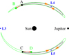 |
Fig. 3 Schematic diagram of the evolution of Jupiter Trojans as a consequence of an outward migrating Jupiter with a speed |


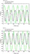 |
Fig. 4 Time evolution of the resonant angle σ for the L4 (panel a) and L5 (panel b) test Trojans starting symmetric tadpole orbits, given initial σ = 90° and σ = 270° (i.e. σ = −90°), respectively. In the case of a non-migrating Jupiter, the σ evolution of these two objects are nicely symmetric, as indicated by the black curves. In the case of an outward migrating Jupiter with the speed of |


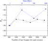 |
Fig. 5 For the case of ΔaJ = 0.12 in Table 1 (highlighted in bold), the variation of the L4-to-L5 number ratio R45 with larger numbers of test Trojans for each swarm (black curve) and longer integration times (blue curve). For reference, a horizontal dashed line is plotted at R45 = 1.6, which corresponds to the unbiased number asymmetry of Jupiter Trojans. |
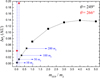 |
Fig. 6 Migration amplitude ΔaJ of Jupiter as a function of the FFP’s mass mFFP in the scenario of the close encounter. The values of mFFP are given in units of Jupiter masses mJ. For reference, less massive FFPs are indicated by their mass values in units of Earth masses mE. The phase angles θ of Jupiter are taken to be: (i) the specific value of θ* = 249° (black symbols); (ii) another representative value of 266° (red symbols). The third parameter of the system, d, is the same as before ( |

2.4 Effects of FFP’s parameters
It is probable that the parameters of the FFP would affect the jumping-Jupiter scenario and the extent of the L4–L5 asymmetry would vary accordingly. In what follows, we evaluate the relative importance of the FFP’s mass mFFP and orbital inclination iFFP, which could be significantly different from what we adopted before (i.e. mFFP = mJ and iFFP = 0º).
2.4.1 FFP’s mass
An important contributor to Jupiter’s migration amplitude ΔaJ is the mass mFFP of the passing-by FFP. Although mFFP is taken to be of the order of mJ in the literature (Varvoglis et al. 2012; Parker et al. 2017; Goulinski & Ribak 2018), as well as in our previous model, this mass value may vary within quite a large range. Indeed, FFPs could have masses up to about 13 Jupiter masses and down to only a few Earth masses (Melita et al. 2008).
Similar to the model constructed for the process of Jupiter jumping as described in Sect. 2.2, we perform some extra runs by choosing different values of mFFP in the range of 10 mE to 5 mJ, where the Earth mass mE is about 0.003 mJ. The other two parameters  and θ = θ* = 249º are kept the same. The results are summarised in Fig. 6, as shown by the black symbols. From left to right, the four stars indicate the cases of mFFP = 10, 50, 100, and 200 mE and the four squares indicate the more massive FFPs with mFFP = 1–5 mJ. We can see that, for mFFP < 1 mJ, the migration amplitude of Jupiter depends nearly linearly on the FFP’s mass, that is, ΔaJ ∝ mFFP. This is easy to understand that the Newtonian gravitational acceleration in the motion of Jupiter is proportional to the mass of the perturber FFP. We further note that, when mFFP is equal to or greater than 2 mJ, the value of ΔaJ seems not to follow the linear increase anymore. This is because the much stronger perturbation of such massive FFP would induce very different geometric configuration of the Jupiter-FFP encounter (e.g. the minimum relative distance). However, according to Table 1, only the most massive FFPs with mFFP ≳ 2 mJ can produce ΔaJ ≳ 0.12, leading to the required L4–L5 asymmetry of R45 ~ 1.6.
We now take a look in Fig. 6 at the cases of the smallest masses of mFFP = 10 and 50 mE, which are highlighted by the vertical dashed lines. For the considered θ = 249º, we find the resulting ΔaJ to be only about <0.02 AU (see the two leftmost black stars), which seems too small to generate the current L4-L5 asymmetry as Table 1 suggests that ΔaJ > 0.12 AU is needed. Bear in mind that, the strongest perturbation of the FFP happens for Jupiter with the initial phase angle θ somewhat larger than 249º, as shown in Fig. 2. When we adjust θ to be 266º and redo the simulations, we find that, for mFFP = 10 and 50 mE, the values of ΔaJ increase to 0.04 and 0.19 AU, respectively (see the red stars in Fig. 6). Accordingly, we propose that ΔaJ could always reach a value of >0.19 AU for mFFP from ~50 mE to a few mJ, since the gravitational effect of the FFP on Jupiter is stronger at larger mFFP. We want to note that, in practice, it is meaningless to consider the cases of θ > 266º, as the motion of Jupiter could become chaotic due to the extremely close encounter between Jupiter and the FFP.
At this point, we conclude that a sub-Saturn or Jupiter-like FFP (i.e. with tens to hundreds of times the mass of Earth) can induce ΔaJ ≳ 0.12 AU that can explain the L4–L5 number asymmetry of Jupiter Trojans, but the less massive super-Earth FFP (i.e. with a few Earth masses) may fail to do so. In addition, we have to point out that in all these cases, Jupiter ends on a nearly circular orbit with eccentricity eJ < 0.05.
2.4.2 FFP’s inclination
So far, we have considered the FFP travelling on a parabolic orbit in the same plane as Jupiter’s orbit, near the invariable plane of the Solar System (Li et al. 2019). It is, however, more likely that the FFP penetrated the Solar System on an inclined orbit.
By looking at Fig. 1, in order to incline the orbital plane of the FFP, we can carry out a rotation about the y-axis through a positive angle iFFP. Such transformation can be represented by introducing the 3 × 3 rotation matrix
 (18)
(18)
and consequently the initial conditions of the FFP given in Eq. (4) are modified as
 (19)
(19)
and
 (20)
(20)
Figure 1 shows that the minimum distance between Jupiter and the FFP occurs at the location of the FFP’s perihelion on the positive x-axis. One can easily picture that, when the FFP’s inclination increases by rotating its orbit about the y-axis, the FFP’s perihelion moves away from Jupiter’s orbital plane, and accordingly the minimum distance between these two planets becomes larger. As a result, the gravitational acceleration on Jupiter caused by the FFP is weaker and the migration amplitude ΔaJ should be smaller. However, the duration of the perihelion passage of the FFP can hardly change and thus the timescale of the close encounter between Jupiter and the FFP would be still around 10 yr. Accordingly, Jupiter’s outward migration slows down, inducing less prominent number asymmetry of the L4 and L5 Trojans.
When the FFP’s orbital plane shifts as the inclination iFFP increases, the z-coordinate of its perihelion is given by
 (21)
(21)
where the semilatus rectum p of the FFP’s parabolic orbit is adopted to be  a as before. It means that the minimum distance betweenp Jupiter and the FFP’s perihelion would not be smaller than
  . We then think that, if the orbital plane of the FFP is elevated along the positive z-axis by a magnitude of
  b, the weakened perturbation on Jupiter may be compensated.
The results of our simulations with different values of iFFP are presented in Table 3. Since the timing of the close encounter is similar to the planar case, according to Fig. 2, we choose the phase angle of Jupiter to be θ = 260°, which can amplify the migration amplitude ΔaJ for Jupiter but would not induce chaotic evolution. For the FFP moving on the original orbit starting with the positions and velocities provided by Eqs. (19) and (20) (i.e. for  ), we can see that ΔaJ decreases monotonically with larger iFFP. At iFFP ≥ 20°, ΔaJ goes down to a value below 0.12 AU, which serves as the lower limit of the migration amplitude of Jupiter that could produce the Trojan number asymmetry of R45 ≳ 1.6 according to the results shown in Table 1.
When the FFP’s orbital plane is moving upwards along the z-axis, that is for  , we find that ΔaJ would indeed become larger (see Table 3). For instance, at iFFP = 40°, we have ΔaJ = 0.10 AU and 0.27 AU when
  is set to be
  and
and  , respectively. Thus, a proper
  between these two values can be found to give ΔaJ > 0.12, to account for the number ratio of R45 ~ 1.6 of Jupiter Trojans. We would like to note that, when
  , the minimum distance between Jupiter and the FFP is about
  . Such a large mutual distance indicates that the gravitational interaction would be extremely small, characterised by ΔaJ = 0.02 AU. But when
  , we find that the said minimum relative distance decreases to only about
  , and consequently Jupiter’s migration amplitude ΔaJ can be much larger, of 0.27 AU. Therefore, the required strength of the FFP’s perturbation can be well met in this circumstance.
However, for a more inclined FFP with iFFP = 50°, there seems to be no significant increase in ΔaJ when  increases from 0 to
  , as ΔaJ is always of the order of ≤0.05 AU. This could be due to the fact that, when iFFP exceeds 45°, the acceleration caused by the FFP along the velocity of Jupiter in the x – y plane becomes smaller than that along the z direction. In addition, for an even larger value of
  , the relative distance between Jupiter and the FFP could reduce to be so small that Jupiter would experience the chaotic evolution because of an extremely close encounter with the FFP.
In summary, in order to explain the unbiased L4–L5 number asymmetry of R45 ~ 1.6, the FFP that invaded the Solar System should have an inclination with respect to Jupiter’s orbital plane at the level of ≲40°. We need to clarify that such an inclined FFP could excite Jupiter’s orbital eccentricity eJ and inclination iJ, but they are always as small as <0.04 and ≲2°, respectively, as shown in the last two columns in Table 3. According to our results in Li et al. (2023), such small eJ and iJ have little effect on the L4–L5 asymmetry in the jumping-Jupiter model.
Excitation of Jupiter’s orbit (i.e. the migration amplitude ΔaJ, the final eccentricity eJ and inclination iJ) within the context of a FFP approaching Jupiter.
3 Direct case: FFP traversing the L5 region
As we conjectured in the introduction, if a FFP once traversed the L5 region, it could deplete a number of local Trojans, while the L4 Trojans would not be affected due to large relative distances (i.e. at the level of the distance between the L4 and L5 point). Such a direct influence of the FFP on the Jupiter Trojans may also induce the L4–L5 number asymmetry. Therefore, we would like to investigate whether this mechanism could explain the required extent of the asymmetry of R45 ~ 1.6.
3.1 The control model
In Sect. 2, in order to achieve the close encounter between Jupiter and the FFP, we determined the initial position phase θ of Jupiter to be θ* (see Eq. (13)). Accordingly, one can make the FFP approach the L5 point, of which Jupiter is 60° ahead, by simply adopting θ = θ* + 60°. Given the same mass and orbit of the FFP (i.e. mFFP = mJ,  ), the deduced parameter θ* = 249° implies the new θ = 309°. In order to simulate accurately the perturbation of the FFP at the time of its perihelion passage, we employ again the RKF algorithm to integrate a system consisting of the Sun, Jupiter, a FFP and two swarms of test Trojans. For either the L4 or L5 swarm, there are 500 objects; the major difference is that, we choose a rather small Δσ0 of 0–40° according to the observed Jupiter Trojans.
As it was noted before, the motions of Jupiter and the FFP in numerical simulations could be somewhat different from our theoretical prediction due to their mutual interactions. Here, we find that when the FFP arrives at its perihelion, the angular difference from Jupiter’s location is about 40°, indicating that the L5 point is still 20° behind the FFP. It suggests that we need to increase the angular position of the L5 point by 20°, equivalently, we increase Jupiter’s initial position phase θ from 309° to 330°. Under such a setting, the FFP can indeed come close to the L5 point around its perihelion and possibly scatter a large number of the local Trojans. We integrate the system for 300 yr, after which the FFP has already been far away from Jupiter’s orbit as it reaches a heliocentric distance of >  . Therefore, the FFP will never perturb Jupiter Trojans again on its way leaving the Solar System.
In the subsequent evolution, only Jupiter and its Trojan population orbit the Sun in the system. For the sake of saving computational time, we instead use the swift_rmvs3 integrator to continue the system’s evolution for another 1 Myr, without the FFP that has already left. At the end of the integration, we identify 269 L5 Trojans surviving on the tadpole orbits, while for the L4 swarm, since its population is always at great distances away from the FFP, all of the 500 members have survived. With this difference, we get a number ratio of R45 = 1.86. Therefore, it is entirely plausible that the observed asymmetry of R45 = 1.6 can be obtained if the perturbations of the FFP on the L5 Trojans are a bit weaker, for instance, in the case of a less massive FFP or a larger encounter distance.
For the Jupiter Trojans, besides explaining the current leading-to-trailing number ratio, the mechanism of a FFP invading the L5 region also works well in retaining the Trojans’ small resonant amplitudes, as shown in Fig. 7. When the FFP penetrates deeply in the L5 region, not all of the local Trojans have the chance to experience close encounters with the FFP and some objects can remain on the unexcited tadpole orbits. These survivors may have their resonant amplitudes nearly unchanged, mainly below 30° as the observation tells us. As for the L4 Trojans, surely they would keep the original resonant amplitude distribution due to the absence of strong perturbations from the FFP. Therefore, this new model could have an additional advantage of reproducing the current observed features of Jupiter Trojans.
3.2 Effects of the FFP’s parameters
As shown above, in the direct case, a FFP that traversed the L5 region once can well account for the number asymmetry of Jupiter Trojans, given its mass mFFP = mJ and inclination iFFP = 0° (i.e. in the same plane of Jupiter’s orbit). Similar to what we did in Sect. 2, it is also of great significance to investigate whether such direct mechanism could be applied to a less massive or more inclined FFP.
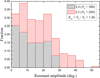 |
Fig. 7 Distribution of resonant amplitudes for surviving L4 (black) and L5 (red) Trojans in the model of a Jupiter mass FFP traversing the L5 region. The final L4-to-L5 number asymmetry can reach a value of R45 = 1.86 (see legend within figure). Besides, a considerable fraction of these simulated Trojans have resonant amplitudes smaller than 30°, similar to the observed objects. |
Statistics of surviving test Trojans in the model of FFP traversing the L5 region.
3.2.1 FFP’s mass
Considering the control model constructed in Sect. 3.1, we first reduce the FFP’s mass mFFP from 1 mJ to 100 mE, while keeping other system parameters the same. Then we simulate again the process of FFP invading the L5 region. As reported in Table 4 (the first two rows), the L4 Trojans are still not affected at all, but there are much more L5 Trojans that could survive, leading to a decrease in the leading-to-trailing number ratio R45 from 1.86 to 1.12.
Bearing in mind that, besides mFFP, the parameters d and θ are also adjustable. In Sect. 2, we chose d = 13  to avoid the collision between the FFP and Jupiter, since d = 12. 8
  yields a FFP’s perihelion located just on the orbit of Jupiter. But here we can adopt d = 12.8
  to let the FFP penetrate the centre of the L5 region and accordingly, we revise the value of θ which describes the phase angle of Jupiter as well as of its Trojan population. Table 4 (the last three rows) shows that, given d = 12. 8
  , the FFP with mFFP ≥ 50 mE is capable of depleting a sufficiently large number of L5 Trojans when it travels into this swarm and the resulting number ratio R45 could reach the value of >1.6, to account for the current asymmetry problem. A much smaller FFP with mFFP = 10 mE, however, does not work no matter how we adjust the values of d and θ. It is quite interesting to point out that, similar to what we found in the jumping-Jupiter model (see Sect. 2.4), the mechanism of FFP invading the L5 Trojans also needs a sub-Saturn FFP at least.
Concerning the L4 Trojans, as seen in Table 4, we notice in a couple of cases that N4 is slightly smaller than the number of initial test Trojans (i.e. = 500). This may be due to the fact that since the FFP is started with d = 12.8  and having its perihelion just on Jupiter’s orbit, it could pass by the L4 region from a distance, not up close, and consequently a tiny fraction of the local Trojans could be removed. Nevertheless, such a small decrease in the number of the L4 Trojans does not affect our results at all.
3.2.2 FFP’s inclination
In analogy to the investigation of different inclinations iFFP of the FFP concerning the jumping Jupiter model in Sect. 2.4.2, here, we evaluate the capability of an inclined FFP to directly deplete the L5 Trojans. In order to achieve the largest perturbation of the FFP when it goes towards the L5 point, the three system parameters mFFP, d, and 0, are respectively adopted to be 1 mJ, 12.8  , and 330° according to our simulations performed in the previous subsection. The results are presented in Table 5.
We first consider the FFP starting with the initial conditions given in Eqs. (19) and (20). In this case, the FFP moves on the original trajectory without any elevation of its orbital plane along the z-axis, indicated by  . As shown in Table 5, the leading-to-trailing number ratio of surviving Trojans decreases from R45 = 2.94 at iFFP = 0° to R45 = 1.87 at iFFP = 10°. Furthermore, at iFFP = 20°, the value of R45 is nearly equal to 1, it means that the number asymmetry has almost disappeared. Therefore, the strength of the FFP’s perturbation on the L5 Trojans weakens very quickly as iFFP becomes higher. We would like to remark that, for the same planar case of iFFP = 0°, the number ratio of R45 = 2.94 given in Table 5 is much larger than the value of 1.86 from the control model. This is because the perturbation of the FFP is stronger due to a smaller d = 12.8
  adopted here.
Next, we lift up the FFP’s orbital plane along the positive z-axis and then the perihelion of the FFP would be closer to the orbital plane of the Trojan population. This way, at high iFFP, the FFP’s perturbation on the L5 Trojans can be partly offset by increasing  (> 0). Table 5 shows that, given proper values of
  , the unbiased number asymmetry of R45 ~ 1.6 can always be achieved for a FFP with inclination iFFP up to as high as 60°. We then suppose that the chance of a FFP entering the Solar System at an inclination within such a wide range of iFFP = 0–60° should not be extremely low. As we only aim in providing a new mechanism to explain the number asymmetry problem of Jupiter Trojans, the possibility of a more inclined FFP with iFFP > 60° will not be explored any further.
Observations show that Jupiter Trojans have inclinations up to about 40°–50°. A plausible explanation of the inclination distribution of the Trojans is the ‘chaotic capture’. During an early instability of the Solar System, the planetesimals were stirred up to high-inclination orbits by the giant planets, and captured into Jupiter’s Lagrangian regions afterwards (Morbidelli et al. 2005; Nesvorný et al. 2013). Here we wonder if a highly inclined FFP that once gravitationally influenced the Trojans could reproduce their large inclinations. So we carefully checked the orbits of surviving Trojans from our simulations, but no significant inclination excitation has been found, as all these objects end with inclinations ≲2°. We think this outcome is reasonable, otherwise the L4 and L5 swarms would have quite different inclination distributions because only the latter is strongly perturbed by the FFP in our model.
4 Conclusions and discussion
In Li et al. (2023) we investigated the number asymmetry of Jupiter Trojans. That dynamical model only took into account the celestial bodies from within our Solar System. Here, we extend this study by considering the invasion of a FFP from interstellar space. On one hand, the FFP could perturb Jupiter’s motion and consequently affect the evolution of the Trojan asteroids in an indirect way. On the other hand, the FFP could directly interact with the Trojans themselves. For both cases, we explored the possibilities of explaining the unbiased L4-to-L5 number ratio of R45 ~ 1.6.
In the indirect case, we consider a jumping-Jupiter that is accelerated via the close encounter with a FFP. We construct the invasion of a Jupiter mass FFP on a parabolic orbit with perihelion outside Jupiter’s orbit, and then investigate the FFP’s gravitational effect on the outward migration of Jupiter. The results show that Jupiter’s migration amplitude ΔaJ could vary in the range of (0, 0.3] AU depending on how deep the close encounter is; while the migration timescale Δt is always of the order of 10 yr, determined by the fast pass-by process of the FFP. Accordingly, Jupiter’s migration speed  could reach a value up to 0.03 AUyr−1. Because At is nearly a constant, the speed
  can be solely characterised by ΔaJ. Then, in the jumping-Jupiter model, we observe the evolution of the L4 and L5 test Trojans starting with symmetric resonant angles of 60º + Δσ0 and −60º − Δσ0, respectively, where Δσ0 is taken to be the same standard setting of 30º–80º as in Li et al. (2023). Given an equal number of initial test Trojans for each swarm, we find that, when ΔaJ = 0.12 AU, the resulting number ratio R45 can be about 1.6. Furthermore, this ratio can continue to go up to a much larger value as ΔaJ increases. Then we are allowed to consider other Δσ0 smaller than the standard setting, which means that the test Trojans are initially closer to the Lagrangian points and the final R45 would be lower due to the more stable L5 swarm. Because in this situation, we can accordingly increase the migration speed
  (i.e. by increasing ΔaJ) to enhance the number asymmetry of the Trojans. When we finally reduce Δσ0 to be as small as 0º–50º, given ΔaJ = 0.2 AU, a number ratio of R45 ~ 1.6 can also be obtained to explain the unbiased number asymmetry of Jupiter Trojans.
It is very important to point out the fundamental difference between our previous work and this one, concerning the jumping-Jupiter model. In Li et al. (2023), Jupiter’s migration speed  is always lower than a critical value of
  AU yr−1. Under that condition, although the L4 region contracts and the L5 region expands, both of them can exist. As a result, the faster migration of Jupiter would induce more stable L4 Trojans and fewer stable L5 Trojans, and accordingly the L4-to-L5 number ratio R45 increases. But, in this work, the jumping-Jupiter has a speed of >0.01 AUyr−1, which is higher than the value of
  . As a consequence, during the outward migration of Jupiter, the two Lagrangian points L3 and L4 merge, and the L4 Trojans temporarily switch to the horseshoe orbits and move towards L3. When Jupiter’s migration ceases within about 10 yr, the L4 point reappears and the surrounding objects come back to tadpole orbits but possess larger resonant amplitudes. So much differently from Li et al. (2023), the faster migration of Jupiter would induce fewer stable L4 Trojans due to the resonant amplitude enlargement, as a larger population of this swarm would be ejected eventually. As for the L5 Trojans, their tadpole orbits can always exist but would become considerably wider due to such fast migration of Jupiter. Taken together, although both the Trojan swarms have their resonant amplitudes increased, the L4 one suffers less excitation in the resonant amplitude and has more stable Trojans that could survive. Therefore, the resulting number ratio R45 can be at the level of 1.6 or even larger. More interestingly, we find that R45 can become infinite when the migration of Jupiter is fast enough, since in this case some L4 Trojans remain stable but all the L5 Trojans have escaped.
At this point, we have achieved a complete understanding of the effect of Jupiter’s fast outward migration on the number asymmetry of the L4 and L5 Jupiter Trojan swarms, for both the cases of migration speeds  below (Li et al. 2023) and above (this work) the critical value of
  AU yr−1. It must be mentioned that, the faster migration of Jupiter with
  does not necessarily require the invasion of a FFP. This process could be attributed to any strong enough acceleration exerted on Jupiter; for instance, an extremely deep close encounter with some ice giant.
However, the mechanism of jumping-Jupiter and L4 and L5 region distortion always encounters the problem that, in the cases where we can obtain R45 ~ 1.6, the simulated Trojans generally have quite larger resonant amplitudes than those of the real Trojans. As we discussed in Li et al. (2023), this issue may be tackled with some dissipation of energy, for example, the mutual collisions. To deal with the inconsistency of the resonant amplitude distribution, we further propose a second mechanism summarised as follows.
In the direct case, we assume that a FFP once traversed the L5 region and thus it could deplete the local Trojans, while the L4 Trojans at large distances were not affected. We find that due to the perturbation of a Jupiter mass FFP, only 53.8% of the L5 Trojans could survive after 1 Myr evolution, but all the L4 Trojans remain on tadpole orbits. This leads to a number ratio of R45 = 1.86, which is potentially capable of explaining the observed asymmetry of R45 ~ 1.6 as long as the FFP is a bit less massive or has a larger encounter distance to Jupiter. In addition, both the L4 and L5 swarms have considerable fractions of simulated Trojans with resonant amplitudes below 30º, similar to the real Jupiter Trojans. As a matter of fact, a similar mechanism was proposed by Nesvorný et al. (2013). But in their model, the value of R45 is found to be about 1.3, which could be due to a smaller invader of the L5 region, that is, an ice giant.
Surely, in either the indirect case or the direct case, the effect of the FFP’s invasion on the number ratio R45 of Jupiter Trojans depends on its parameters, especially the mass mFFP and inclination iFFP. It is very interesting to find that in both cases, in order for the L4–L5 number asymmetry to be explained at the level of R45 ~ 1.6, the FFP could have similar parameter ranges of mFFP from tens of Earth masses to a few Jupiter masses and iFFP as large as 40º. Given such wide ranges of mFFP and iFFP, we suppose that the chance of a proper FFP entering our Solar System should not be extremely low.
Acknowledgements
This work was supported by the National Natural Science Foundation of China (Nos. 11973027, 11933001, 12150009), and National Key R&D Program of China (2019YFA0706601). And part of this work was also supported by a Grant-in-Aid for Scientific Research (20H04617). We would also like to express our sincere thanks to the anonymous referee for the valuable comments.
References
- Di Sisto, R. P., Ramos X. S., & Beaugé, C. 2014, Icarus, 243, 287 [NASA ADS] [CrossRef] [Google Scholar]
- Di Sisto, R. P., Ramos X. S., & Gallardo, T. 2019, Icarus, 319, 828 [NASA ADS] [CrossRef] [Google Scholar]
- Freistetter, F. 2006, A&A, 453, 353 [NASA ADS] [CrossRef] [EDP Sciences] [Google Scholar]
- Goulinski, N., & Ribak, E. N. 2018, MNRAS, 473, 1589 [NASA ADS] [Google Scholar]
- Grav, T., Mainzer, A. K., Bauer, J., et al. 2011, ApJ, 742, 40 [NASA ADS] [CrossRef] [Google Scholar]
- Grav, T., Mainzer, A. K., Bauer, J. M., et al. 2012, ApJ, 759, 49 [NASA ADS] [CrossRef] [Google Scholar]
- Holt, T. R., Nesvorný, D., Horner, J., et al. 2020, MNRAS, 495, 4085 [NASA ADS] [CrossRef] [Google Scholar]
- Jewitt, D. C., Sheppard, S., & Porco, C. 2004, in Jupiter: The Planet, Satellites and Magnetosphere, eds. F. Bagenal, T. Dowling, & W. McKinnon (Cambridge: Cambridge University Press), 263 [Google Scholar]
- Levison, H. F., & Duncan, M. J. 1994, Icarus, 108, 18 [NASA ADS] [CrossRef] [Google Scholar]
- Li, G., & Adams, F. C. 2016, ApJ, 823, L3 [NASA ADS] [CrossRef] [Google Scholar]
- Li, J., & Sun, Y.-S. 2018, A&A, 616, A70 [NASA ADS] [CrossRef] [EDP Sciences] [Google Scholar]
- Li, J., Xia, Z. J., & Zhou L. 2019, A&A, 630, A68 [NASA ADS] [CrossRef] [EDP Sciences] [Google Scholar]
- Li, J., Xia, Z. J., Yoshida, F., et al. 2023, A&A, 669, A68 [NASA ADS] [CrossRef] [EDP Sciences] [Google Scholar]
- Malhotra R. 1995, AJ, 110, 420 [NASA ADS] [CrossRef] [Google Scholar]
- Marzari, F., & Scholl, H. 1998, A&A, 339, 278 [NASA ADS] [Google Scholar]
- Marzari, F., & Scholl, H. 2000, Icarus, 232, 239 [Google Scholar]
- Miret-Roig, N., Bouy, H., Raymond, S. N., et al. 2022, Nat. Astron., 6, 89 [NASA ADS] [CrossRef] [Google Scholar]
- Morbidelli, A., Levison, H. F., Tsiganis, K., & Gomes, R. 2005, Nature, 435, 462 [Google Scholar]
- Murray-Clay, R. A., & Chiang, E. I. 2005, ApJ, 619, 623 [NASA ADS] [CrossRef] [Google Scholar]
- Nakamura, T., & Yoshida, F. 2008, PASJ, 60, 293 [NASA ADS] [CrossRef] [Google Scholar]
- Nesvorný, D. 2018, ARA&A, 56, 137 [CrossRef] [Google Scholar]
- Nesvorný, D., Vokrouhlický, D., & Morbidelli, A. 2013, ApJ, 768, 45 [CrossRef] [Google Scholar]
- Nicholson, S. B. 1961, Astron. Soc. Pac. Leaflets, 8, 239 [NASA ADS] [Google Scholar]
- Ogilvie, G. I., & Lubow, S. H. 2006, MNRAS, 370, 784 [NASA ADS] [CrossRef] [Google Scholar]
- Parker, R. J., Lichtenberg T., & Quanz S. P. 2017, MNRAS, 472, L75 [NASA ADS] [CrossRef] [Google Scholar]
- Shoemaker, E. M., Shoemaker, C. S., & Wolfe, R. F. 1989, in Asteroids II, eds. R. P. Binzel, T. Gehrels, & M. S. Matthews (Tucson: University of Arizona Press), 487 [Google Scholar]
- Sicardy, B., & Dubois, V. 2003, Celest. Mech. Dyn. Astron., 86, 321 [NASA ADS] [CrossRef] [Google Scholar]
- Slyusarev I. G. 2013, Lunar Planet. Sci. 1719, 2223 [Google Scholar]
- Sumi, T., Kamiya, K., Bennett, D. P., et al. 2011, Nature, 473, 349 [Google Scholar]
- Szabó, G. M., Ivezić, Ž., Jurić, M., & Lupton, R. 2007, MNRAS, 377, 1393 [CrossRef] [Google Scholar]
- Varvoglis, H., Sgardeli, V., & Tsiganis, K. 2012, Celest. Mech. Dyn. Astron., 113, 387 [NASA ADS] [CrossRef] [Google Scholar]
All Tables
Statistics of surviving test Trojans within the model of Jupiter’s outward migration.
Excitation of Jupiter’s orbit (i.e. the migration amplitude ΔaJ, the final eccentricity eJ and inclination iJ) within the context of a FFP approaching Jupiter.
Statistics of surviving test Trojans in the model of FFP traversing the L5 region.
All Figures
|
Fig. 1 Schematic diagram of the jumping-Jupiter evolution due to the invasion of a FFP in the co-planar model. Jupiter is initially on a circular orbit (solid circle) around the Sun, with phase angle θ measured anticlockwise from the positive x-axis. The FFP is approaching the Sun-Jupiter system on a parabolic orbit with initial coordinates ( |
| In the text | |
|
Fig. 2 Invading FFP with a distance parameter |
| In the text | |
|
Fig. 3 Schematic diagram of the evolution of Jupiter Trojans as a consequence of an outward migrating Jupiter with a speed |
| In the text | |
|
Fig. 4 Time evolution of the resonant angle σ for the L4 (panel a) and L5 (panel b) test Trojans starting symmetric tadpole orbits, given initial σ = 90° and σ = 270° (i.e. σ = −90°), respectively. In the case of a non-migrating Jupiter, the σ evolution of these two objects are nicely symmetric, as indicated by the black curves. In the case of an outward migrating Jupiter with the speed of |
| In the text | |
|
Fig. 5 For the case of ΔaJ = 0.12 in Table 1 (highlighted in bold), the variation of the L4-to-L5 number ratio R45 with larger numbers of test Trojans for each swarm (black curve) and longer integration times (blue curve). For reference, a horizontal dashed line is plotted at R45 = 1.6, which corresponds to the unbiased number asymmetry of Jupiter Trojans. |
| In the text | |
|
Fig. 6 Migration amplitude ΔaJ of Jupiter as a function of the FFP’s mass mFFP in the scenario of the close encounter. The values of mFFP are given in units of Jupiter masses mJ. For reference, less massive FFPs are indicated by their mass values in units of Earth masses mE. The phase angles θ of Jupiter are taken to be: (i) the specific value of θ* = 249° (black symbols); (ii) another representative value of 266° (red symbols). The third parameter of the system, d, is the same as before ( |
| In the text | |
|
Fig. 7 Distribution of resonant amplitudes for surviving L4 (black) and L5 (red) Trojans in the model of a Jupiter mass FFP traversing the L5 region. The final L4-to-L5 number asymmetry can reach a value of R45 = 1.86 (see legend within figure). Besides, a considerable fraction of these simulated Trojans have resonant amplitudes smaller than 30°, similar to the observed objects. |
| In the text | |
Current usage metrics show cumulative count of Article Views (full-text article views including HTML views, PDF and ePub downloads, according to the available data) and Abstracts Views on Vision4Press platform.
Data correspond to usage on the plateform after 2015. The current usage metrics is available 48-96 hours after online publication and is updated daily on week days.
Initial download of the metrics may take a while.