| Issue |
A&A
Volume 631, November 2019
|
|
|---|---|---|
| Article Number | A68 | |
| Number of page(s) | 15 | |
| Section | Numerical methods and codes | |
| DOI | https://doi.org/10.1051/0004-6361/201936387 | |
| Published online | 22 October 2019 | |
Hydrostatic equilibrium preservation in MHD numerical simulation with stratified atmospheres
Explicit Godunov-type schemes with MUSCL reconstruction
1
Departamento de Aeronáutica, Facultad de Ciencias Exactas, Físicas y Naturales, Universidad Nacional de Córdoba, Argentina
e-mail: This email address is being protected from spambots. You need JavaScript enabled to view it.
2
Instituto de Estudios Avanzados en Ingeniería y Teconología, IDIT-UNC-CONICET, Argentina
Received:
26
July
2019
Accepted:
6
September
2019
Abstract
Context. Many astrophysical processes involving plasma flows are produced in the context of a gravitationally stratified atmosphere in hydrostatic equilibrium, in which strong gradients can exist with gas properties that vary in small regions by several orders of magnitude. The standard Godunov-type schemes with polynomial reconstruction used to numerically solve these problems fail to preserve the hydrostatic equilibrium owing to the appearance of spurious fluxes generated by the numerical unbalance between gravitational forces and pressure gradients.
Aims. The aim of this work is to present local hydrostatic reconstruction techniques that can be implemented in existing codes with Godunov-type methods to obtain well-balanced schemes that numerically satisfy the hydrostatic equilibrium for various conditions.
Methods. The proposed numerical scheme is based on the Godunov method with second order MUSCL-type reconstruction, as is extensively used in astrophysical applications. The difference between the scheme and the standard formulations is only given by calculating the pressure and density Riemann states on each intercell face and by computing the gravitational source term on each cell.
Results. The local hydrostatic reconstruction scheme is implemented in the FLASH code to verify the well-balanced property for hydrostatic equilibrium with constant or linearly variable temperature and constant or variable gravity. In addition, the behavior of the scheme for hydrostatic equilibrium with arbitrary temperature distributions is also analyzed together with the ability to propagate low-amplitude waves and to capture shock waves.
Conclusions. The scheme is demonstrated to be robust and relatively simple to implement in existing codes. This approach produces good results in hydrostatic equilibrium preservation, satisfying the well-balanced property for the preset conditions and strongly reducing the spurious fluxes for extreme configurations.
Key words: methods: numerical / magnetohydrodynamics (MHD) / Sun: atmosphere / Sun: general
© ESO 2019
1. Introduction
Many astrophysical processes involving plasma flows can be modeled using equations of magnetohydrodynamics (MHD). These equations arise from the coupling between equations of fluid mechanics and Maxwell’s equations, and they allow us to model the plasma motion under certain conditions that can be assumed in multiple astrophysical phenomena. Magnetohydrodynamics equations do not have a general exact solution, therefore they have to be solved using alternative techniques. Thus, numerical simulations play a very important role in obtaining solutions for many processes that are modeled by these equations.
The dynamics of the solar atmosphere is often analyzed using MHD numerical simulations to study multiple phenomena that occur there. Some of these phenomena evolve in the context of a very gravitationally stratified medium with strong pressure and temperature gradients (e.g. Aschwanden 2005; Mei et al. 2012; Murawski et al. 2013; Krause et al. 2018). The numerical codes used in these simulations must be able to maintain the hydrostatic equilibrium of the background medium at some precision level so as not to introduce spurious results that affects the actual physical behavior. Sometimes a certain level of spurious accelerations is acceptable so that conventional numerical methods can be used in relatively fine grids, but in other situations it is necessary to minimize the presence of nonphysical velocities, which could mask or significantly alter the studied processes. For this reason, special modifications to the standard numerical schemes have been proposed in order to satisfy the discrete equilibrium in hydrostatic conditions exactly. We emphasize that hydrostatic equilibrium preservation does not only concern stationary problems, but can be a crucial aspect for many dynamic processes that occur in the context of an hydrostatically balanced environment. In these cases, a numerically induced velocity can strongly affect or even completely overlap the studied dynamics leading to erroneous results. Some examples of these phenomena are wave propagation in stratified magnetic atmospheres (Fuchs et al. 2010), low-amplitude wave propagation in helioseismology (Kobanov et al. 2008), or the interaction between coronal and chromospheric waves Krause et al. (2018).
The capability of a scheme to numerically satisfy an equilibrium condition is known as a well-balanced property after the work by Greenberg & Leroux (1996), who introduced this terminology to characterize those schemes that are able to exactly satisfy, in a numerical discrete sense, a defined stationary state. In the particular case of the hydrostatic equilibrium, some well-balanced schemes have been developed to model numerically the variants of that condition (e.g. Botta et al. 2004; Audusse et al. 2004; Felipe et al. 2010; Fuchs et al. 2010; Xing & Shu 2013; Käppeli & Mishra 2014, 2016). Among these, schemes that use a local hydrostatic reconstruction are the simplest since this technique does not require a modification of the system of governing equations nor the central aspects of the standard numerical schemes. This allows for a relatively simple implementation of the method in existing codes with the conventional Godunov-type schemes mostly used in the astrophysical community (e.g. Fryxell et al. 2000; Pen et al. 2003; Ziegler 2004; Mignone et al. 2007).
In this work we choose the local hydrostatic reconstruction approach following the ideas of works by Fuchs et al. (2010), Käppeli & Mishra (2014, 2016). We propose some contributions that allow us to simulate equilibrium atmospheres in more general conditions than the isothermal or isentropic cases, for both constant and variable gravity, without the need to define new variables nor solve additional equations.
The paper is organized as follows. In Sect. 2 we present the governing equations of the MHD problem and we show the analytic conditions of hydrostatic equilibrium. In Sect. 3 we briefly summarize the numerical methods used in this work and discuss the problem of hydrostatic equilibrium preservation for these types of numerical schemes. In Sect. 4 we present an extension of a local hydrostatic reconstruction technique and in Sect. 5 we detail its implementation in the FLASH1 code. Finally, in Sect. 6 we show some results to verify our formulation and in Sect. 7 we present the main conclusions of this work.
2. Governing equations
Considering an ideal plasma (inviscid and without magnetic resistivity), the ideal MHD equations in conservative form and in CGS units are written as
 (1)
(1)
 (2)
(2)
 (3)
(3)
![Mathematical equation: $$ \begin{aligned}&\frac{\partial E}{\partial t} + \nabla \cdot \left[\left(E + p + \frac{B^2}{8\pi }\right){\boldsymbol{u}} - \frac{1}{4\pi }\left({\boldsymbol{u}}\cdot {\boldsymbol{B}}\right){\boldsymbol{B}}\right] = \rho {\boldsymbol{g}} \cdot {\boldsymbol{u}}, \end{aligned} $$](/articles/aa/full_html/2019/11/aa36387-19/aa36387-19-eq4.gif) (4)
(4)
where ρ is the plasma density, u = (u, v, w) is the velocity, B = (Bx, By, Bz) is the magnetic field, p is the thermal pressure, and E is the total energy (per unit volume), i.e.,
where ϵ is the specific internal energy. The vector g = (gx, gy, gz) is the gravitational acceleration.
The set of Eqs. (1)–(4) must be closed by means of an equation of state that links thermal pressure with other thermodynamic variables (p = f(ρ, ϵ)), In addition, the divergence-free condition of the magnetic field (∇ ⋅ B = 0) must be fulfilled everywhere.
The conservative MHD equations constitute a conservation law that expresses the balance between the variation, flux and source term of each conservative variable,
 (5)
(5)
where
![Mathematical equation: $$ \begin{aligned} {\boldsymbol{U}} = \left[ \begin{array}{c} \rho \\ \rho u \\ \rho { v} \\ \rho { w} \\ B_x \\ B_{ y} \\ B_z \\ E \end{array} \right] \end{aligned} $$](/articles/aa/full_html/2019/11/aa36387-19/aa36387-19-eq7.gif) (6)
(6)
is the vector of conservative variables, and
![Mathematical equation: $$ \begin{aligned}&{\boldsymbol{F}} = \left[ \begin{array}{c} \rho u \\ \rho u^2 + p + \frac{B^2}{8\pi } - \frac{B_x^2}{4\pi } \\ \rho u { v} - \frac{1}{4\pi }B_{ y} B_x \\ \rho u { w} - \frac{1}{4\pi }B_z B_x \\ 0 \\ u B_{ y} - { v} B_x \\ u B_z - { w} B_x \\ \left(E + p + \frac{B^2}{8\pi }\right)u - \frac{1}{4\pi }B_x (u B_x + { v} B_{ y} + { w} B_z) \end{array} \right], \nonumber \\&{\boldsymbol{G}} = \left[ \begin{array}{c} \rho { v} \\ \rho { v} u - \frac{1}{4\pi }B_x B_{ y} \\ \rho { v}^2 + p + \frac{B^2}{8\pi } - \frac{B_{ y}^2}{4\pi } \\ \rho { v} { w} - \frac{1}{4\pi }B_z B_{ y} \\ { v} B_x - u B_{ y} \\ 0 \\ { v} B_z - { w} B_{ y} \\ \left(E + p + \frac{B^2}{8\pi }\right){ v} - \frac{1}{4\pi }B_{ y} (u B_x + { v} B_{ y} + { w} B_z) \end{array} \right], \\&{\boldsymbol{H}} = \left[ \begin{array}{c} \rho { w} \\ \rho { w} u - \frac{1}{4\pi }B_x B_z \\ \rho { w} { v} - \frac{1}{4\pi }B_{ y} B_z \\ \rho { w}^2 + p + \frac{B^2}{8\pi } - \frac{B_z^2}{4\pi } \\ { w} B_x - u B_z \\ { w} B_{ y} - { v} B_z \\ 0 \\ \left(E + p + \frac{B^2}{8\pi }\right){ v} - \frac{1}{4\pi }B_z (u B_x + { v} B_{ y} + { w} B_z) \end{array} \right]\nonumber \end{aligned} $$](/articles/aa/full_html/2019/11/aa36387-19/aa36387-19-eq8.gif) (7)
(7)
are the flux vectors in x, y, and z direction in a Cartesian coordinate system. In this case, the source term is only given by the components of the gravitational acceleration
![Mathematical equation: $$ \begin{aligned} {\boldsymbol{S}} = \left[ \begin{array}{c} 0 \\ \rho {g}_x \\ \rho {g}_{ y} \\ \rho {g}_z \\ 0 \\ 0 \\ 0 \\ \rho ({g}_x u + {g}_{ y} { v} + {g}_z { w}) \end{array}\right]\cdot \end{aligned} $$](/articles/aa/full_html/2019/11/aa36387-19/aa36387-19-eq9.gif) (8)
(8)
There are several numerical methods that were specifically developed to solve MHD equations (e.g. Colella & Woodward 1984; Balsara & Spicer 1999; Powell et al. 1999; Gardiner & Stone 2005), which were implemented in many computational codes with different features and capabilities. In general, these codes use some extension of the Godunov method, which is based on the finite volume method (FVM). In this type of scheme the physic domain is subdivided into small control volumes (cells) on each of which the conservation laws of mass, momentum, magnetic flux, and energy must be satisfied, i.e., the balance between the inbound and outbound fluxes of each conservative property, its source term, and its rate of change must be fulfilled on each cell. This integral approach allows us to capture discontinuous solutions such as shocks waves and contact discontinuities that can be present in high energy plasma flows, as regularly occurs in the solar atmosphere (blasts, coronal mass ejections, etc.).
Usually, the main challenge for numerically solving MHD equations lies in the evolution of the magnetic field, which has to satisfy the divergence-free constraint (∇ ⋅ B = 0) at all times. This requirement does not allow the use of direct extensions of fluid codes to solve the MHD equations, since the discrete evaluation of magnetic field gradients introduces artificial divergence even when the initial magnetic field is solenoidal, which violates the law of nonexistence of magnetic monopoles. The non-preservation of the divergence-free condition causes discrepancies between the conservative and primitive forms of the MHD equations. In addition, the Lorentz force is not normal to the magnetic field (Brackbill & Barnes 1980) and the jump conditions through MHD shocks can be incorrect under certain conditions (Tóth 2000). For these reasons, many efforts have been carried out to obtain numerical schemes that hold the magnetic field divergence in very small levels throughout the simulation. In the Godunov-type schemes three methods to attack this problem can be distinguished: “clean” the magnetic field of any spurious divergence after each time step using a Hodge projection (Gardiner & Stone 2005); expand the set of governing equations, by incorporating an equation for the divergence evolution designed to eliminate the error accumulation (Powell et al. 1999); and write the finite difference equations for the magnetic field such that the magnetic flux is explicitly conserved to preserve the divergence-free condition at the discretization level (e.g. Evans & Hawley 1988; Lee & Deane 2009). With some of these techniques and some Riemann solver developed for MHD equations (e.g. Powell 1994; Cargo & Gallice 1997; Gurski 2004; Miyoshi & Kusano 2005), the numerical solution of Eqs. (1)–(4) is obtained in a similar way as the gas dynamic equations. In our study, we are interested in the “gas dynamic part” of the MHD problem, since we are proposing a methodology to satisfy hydrostatic equilibrium in atmospheres at rest, which is a fluid problem. Therefore, even though we only consider the gas dynamic variables in the MHD equations, this approach can be applied on any Godunov-type MHD code. In addition, for simplicity we considered a 2D domain taking into account that the extension to 3D problems is trivial.
Then, for our analysis we used the 2D Euler equations, which can be viewed as a particular case of Eqs. (1)–(4) when the magnetic field is zero (B = 0). The resulting equations after eliminating the terms associated with the magnetic field and the components in the z-direction are written as
 (9)
(9)
 (10)
(10)
 (11)
(11)
The vector of conservative variables and the vectors of fluxes for the 2D Euler equations are written as
![Mathematical equation: $$ \begin{aligned} {\boldsymbol{U}} = \left[ \begin{array}{c} \rho \\ \rho u \\ \rho { v} \\ E \end{array} \right], \quad {\boldsymbol{F}} = \left[ \begin{array}{c} \rho u \\ \rho u^2 + p \\ \rho { v} u \\ (E + p)u \end{array} \right], \quad {\boldsymbol{G}} = \left[ \begin{array}{c} \rho { v} \\ \rho u { v} \\ \rho { v}^2 + p \\ (E + p){ v} \end{array} \right]\cdot \end{aligned} $$](/articles/aa/full_html/2019/11/aa36387-19/aa36387-19-eq13.gif) (12)
(12)
In order to simplify the analysis, the coordinate system is oriented so that the gravitational acceleration direction is parallel to the y coordinate pointing downward. Thus, for a gravity vector g of magnitude g, the gravitational source term is
![Mathematical equation: $$ \begin{aligned} {\boldsymbol{S}} = \left[ \begin{array}{c} 0 \\ 0 \\ -\rho {g} \\ -\rho {g} { v} \end{array} \right]\cdot \end{aligned} $$](/articles/aa/full_html/2019/11/aa36387-19/aa36387-19-eq14.gif) (13)
(13)
The nonconservative form of the system (9)–(11) is written in terms of the Jacobian matrices Ax and Ay, and the vector of primitive variables V as
 (14)
(14)
where
![Mathematical equation: $$ \begin{aligned}&{\boldsymbol{V}} = \left[ \begin{array}{c} \rho \\ u \\ { v} \\ p \end{array} \right], \quad \mathbf A _x = \left(\frac{\partial {\boldsymbol{U}}}{\partial {\boldsymbol{V}}}\right)^{-1} \frac{\partial {\boldsymbol{F}}}{\partial {\boldsymbol{V}}}, \quad \mathbf A _{ y} = \left(\frac{\partial {\boldsymbol{U}}}{\partial {\boldsymbol{V}}}\right)^{-1}\frac{\partial {\boldsymbol{G}}}{\partial {\boldsymbol{V}}}, \nonumber \\&{{\boldsymbol{S}}_V} = \left[ \begin{array}{c} 0 \\ 0 \\ -{g} \\ \rho {g} { v} (\gamma - 1) \end{array} \right]\cdot \end{aligned} $$](/articles/aa/full_html/2019/11/aa36387-19/aa36387-19-eq16.gif) (15)
(15)
In the hydrostatic equilibrium condition the gravitational forces are balanced by the pressure forces so that the fluid remains at rest if there are no perturbations. This condition implies that the velocity in the gravity direction is zero (v = 0 in this case) and pressure and density vary only in that direction according to the height equation
 (16)
(16)
The solution of the height equation is given by the prescribed distribution of one of the thermodynamic variables that has to be known to obtain a unique solution for the equilibrium. In the modeling of stellar atmospheres it is usual to prescribe the radial temperature distribution, since this profile can generally be estimated. In the particular case of the Sun, there are several models for the temperature variation in the different layers of the solar atmosphere (Aschwanden 2005). The link between the temperature and height Eq. (16) is given by the equation of state. Taking into account that the assumption of an ideal gas atmosphere is widely adopted in the study of the solar atmosphere, we focused our analysis on this model since it is a simple and reasonable supposition that allowed us to obtain explicit formulations for the numerical scheme. Therefore, for the equation of state of ideal gases we have
 (17)
(17)
where R is the particular gas constant (relation between the universal gas constant and the gas molar mass) and γ is the specific heats relation. With this assumption, Eq. (16) reads
 (18)
(18)
where the distribution T(y) is known. Integrating the last expression gives
 (19)
(19)
where p0 is a reference pressure that is known at the reference height y0.
Equation (19) gives the hydrostatic pressure distribution for a given temperature profile T(y) for an ideal gas atmosphere. In those regions where the velocity is zero and the thermodynamic variables satisfy Eq. (19), the fluid remains at rest if there are no perturbations. Under certain conditions such as strong pressure gradients, large height scales, or in long-lasting phenomena, the conventional Godunov-type numerical schemes fail to preserve the hydrostatic equilibrium; this is because the exponential variation of pressure in the gravity direction cannot be captured by the classical reconstruction-evolution methods even when they are of high order. As a consequence, unbalanced momentum fluxes arise in the gravity direction, which induce spurious vertical velocities that constantly increase with the advance of time. Although the magnitude of these spurious velocities can be reduced, thereby enhancing the grid resolution (provided that the implemented method is convergent), in some problems this strategy is not possible because of the strong penalty in computational cost that implies the excessive increment of computing cells.
3. Godunov-type numerical schemes
Co-located FVMs assume that inside each control subvolume, i.e., inside each cell, the variables are constant and equal to an averaged quantity. By definition, inside a cell identified by the subindices i, j in a structured Cartesian grid of rectangles of dimension Δx × Δy (see Fig. 1), the discrete vector of conservative variables for a given time tn is written as
 (20)
(20)
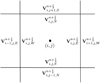 |
Fig. 1. Definitions for a generic cell i, j in a structured Cartesian grid. |
where xi and yj are the coordinates of the cell center.
The evolution of the discrete variable Ui, j from the time tn to the time tn + 1 = tn + Δt is obtained by considering the integral form of the conservation law (5) applied on the control volume defined by the corner points  and
and  as
as
 (21)
(21)
where the discrete fluxes are averaged over the cell faces of coordinates  and
and  and through the time interval tn ≤ t ≤ tn + Δt, i.e.,
 (22)
(22)
3.1. Numerical flux
Typically, the averaged fluxes are approximated by numerical fluxes  and
and  , which must satisfy the conservation property. In the Godunov-type schemes the numerical fluxes are evaluated by constructing Riemann problems (RP) at the interfaces of adjacent cells, where discontinuities can exist owing to the difference between the averaged quantities of each cell. The variable values on each side of the intercell boundary, namely, the RP states, are defined by some reconstruction technique that is used to extrapolate the cell-centered values of the variables to the cell faces. With the solution of the RP the numerical fluxes are evaluated by means of the physic fluxes (e.g. Toro 2009)
 (23)
(23)
where  and
and  are the solutions of the RP on faces normal to the x-direction and the y-direction, respectively, i.e.,
The variable averaging over the time interval (step  ) depends on the implemented temporal integration scheme. The subindices E, W, N, and S (east, west, north, and south) denote the relative positions of the cell faces with respect to the cell center, according to the nomenclature usually used (see Fig. 1).
The way in which we extrapolated the cell-centered values to the faces to construct the RPs defines the spatial approximation order of a Godunov-type scheme. The MUSCL (monotone upwind scheme for conservation laws) schemes, initially proposed by van Leer (1979) reconstruct the variable inside the cell using the values at neighboring cells to calculate an interpolating polynomial, whose order is given by the number of surrounding cell values used in the calculation. This polynomial, whose integration over the cell must satisfy the definition (20) to verify the conservation property, allows us to evaluate the reconstructed variables at face positions. In addition, a flux limiter (FL) function has to be used to preserve the monotonicity of the solution (Toro 2009).
The solution of the RPs at each interface is obtained using some approximate Riemann solver, which must satisfy the consistency property that requires that in a constant state through the interface, the numerical flux has to be equal to the physics flux. This means that the solution of the Riemann solver for a constant state has to be equal to the constant values. On the other hand, in many applications it is also necessary that the Riemann solver can capture contact discontinuities, which implies that the numerical flux for a constant pressure state with zero velocity normal to the face only produces a flux momentum component that is normal to the face and equal to the pressure, i.e.,
![Mathematical equation: $$ \begin{aligned}&{\boldsymbol{F}}\left(\mathrm{RP} \left\{ \left[\begin{array}{c} \rho _{E^-} \\ 0 \\ 0 \\ p \end{array}\right],\left[\begin{array}{c} \rho _{W^+} \\ 0 \\ 0 \\ p \end{array}\right] \right\} \right) = \left[\begin{array}{c} 0 \\ p \\ 0 \\ 0 \end{array}\right],\nonumber \\&{\boldsymbol{G}}\left(\mathrm{RP} \left\{ \left[\begin{array}{c} \rho _{N^-} \\ 0 \\ 0 \\ p \end{array}\right],\left[\begin{array}{c} \rho _{S^+} \\ 0 \\ 0 \\ p \end{array}\right] \right\} \right) = \left[\begin{array}{c} 0 \\ 0 \\ p \\ 0 \end{array}\right]\cdot \end{aligned} $$](/articles/aa/full_html/2019/11/aa36387-19/aa36387-19-eq35.gif) (24)
(24)
In other words, in a constant pressure state with zero velocity, the numerical flux has to be equal to the physical flux independent of the density values on each side of the interface. In general, this property is very important to improve the hydrostatic equilibrium preservation of conventional Godunov-type schemes.
3.2. Source terms
The numerical evaluation of the source term is also made by means of an averaging over the cell and the time interval, i.e.,
 (25)
(25)
For the particular case in which the source term is only due to gravity, which does not depend on time, the averaging is usually replaced by the cell-centered evaluation of the gravitational acceleration, i.e.,
![Mathematical equation: $$ \begin{aligned} {\boldsymbol{S}}^{n+\frac{1}{2}}_{i,j} = \left[ \begin{array}{c} 0 \\ 0 \\ -\rho _{i,j}^{n+\frac{1}{2}} {g}({ y}_j) \\ -(\rho { v})_{i,j}^{n+\frac{1}{2}} {g}({ y}_j) \end{array} \right]\cdot \end{aligned} $$](/articles/aa/full_html/2019/11/aa36387-19/aa36387-19-eq37.gif) (26)
(26)
This expression is the same as Eq. (25) when gravity is constant and is approximate to that average for variable gravity.
3.3. Hydrostatic equilibrium preservation
In this section we describe some problems concerning the hydrostatic equilibrium preservation in standard Godunov-type schemes. For the analysis, we start from a hydrostatic configuration where the pressure and density distributions satisfy Eq. (16) and the velocity is zero everywhere (u = 0). Naturally, this is a stationary problem, but we want to know how explicit Godunov-type methods, such as those usually implemented in astrophysical simulation, behave under this situation.
Numerically, the hydrostatic condition manifests as follows: Taking into account that there are no source terms acting in that x-direction and that hydrostatic pressure and density are constant with respect to x in our model with gravity parallel to the y-direction, the condition of zero velocity implies that the net flux  is zero; this happens in any trivial problem with constant variable distributions without source terms. On the other hand, in the y-direction pressure and density are not constant but present an exponential decay with height, thus the net flux
  is not zero for u = 0. The hydrostatic configuration remains at rest only if the gravitational source terms exactly cancel the net flux, i.e.,
 (27)
(27)
For the hydrostatic equilibrium to be numerically preserved, Eq. (27) should be reduced to a discrete form of the height Eq. (16) so that the velocity remains zero and the thermodynamic variables are unchanged. This implies that the y-momentum component of the net numerical flux must be canceled by the corresponding source term, i.e.,
 (28)
(28)
where  should be the only non-zero components of the numerical fluxes
  .
.
Equation (28) shows the reason by which standard Godunov-type schemes cannot preserve a hydrostatic equilibrium condition. Firstly, we see that the y-momentum component of the numerical flux  must only be due to pressure since velocity has to be zero. This requires that the RP solution on faces normal to y should not produce non-zero velocity components in that direction (i.e.,
  ) in order for Eq. (27) to reduces to Eq. (28). Secondly, the numerical evaluation of the source term −ρg at each cell must be equal to the y-momentum component of the net numerical flux divided by Δy.
For the first aspect, we need to construct a RP with a constant pressure state through the cell face when the hydrostatic equilibrium is satisfied, with which we can obtain a solution of the form of Eq. (24) for flux  . This means that, under a hydrostatic equilibrium condition, the extrapolation in the y-direction of the pressure cell-centered values to a face should give the same value either using the below or above cell (i.e.,
  ). Conventional polynomial MUSCL reconstruction techniques do not allow us to produce such a constant pressure state because they are not able to capture the exponential decay of the variable. Consequently, a pressure jump is generated at the interface (see Fig. 2 for the examples of a first and second order reconstruction), which induces a non-zero velocity. We must note that an increase of the reconstruction order using higher order polynomials, even though it reduces the difference between the extrapolated pressures on each side of the interface, always presents errors with respect to the actual exponential distribution. The strategy usually used to reduce the spurious velocities caused by these errors in conventional codes is to increase the grid resolution, but sometimes this is not possible owing to the strong impact on computational cost that is generated under certain conditions (for instance, very large pressure gradients in small regions of the domain).
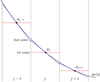 |
Fig. 2. First (red lines) and second (blue lines) order standard reconstruction in a hydrostatic pressure distribution. The solid black line represents the equilibrium hydrostatic pressure p0(y). |
The second aspect, related to the numerical evaluation of the gravitational source term, also introduces errors in the hydrostatic equilibrium preservation of standard schemes. It is clear that the y-momentum component of the source term evaluated by Eq. (26) is not equal to the right-hand side of Eq. (28) in the general case. Hence, even if we could satisfy the required conditions for the left-hand side of the discrete height equation, the numerical scheme would not preserve the hydrostatic equilibrium if the source term  is not correctly evaluated. Naturally, these errors can be reduced by improving the grid resolution but, as mentioned, this option is not always available.
As expressed in the previous paragraphs, it is clear that the conventional Godunov-type finite volume schemes are not able to reproduce a discrete hydrostatic equilibrium condition exactly. A good analysis referring to this issue is found in Zingale et al. (2002), who studied the effect of the scheme type, the treatment of boundary conditions, and the influence of the grid resolution in the modeling of gravitational stratified mediums.
As we mentioned in the Introduction, a well-balanced numerical scheme is able to numerically reproduce a given stationary solution. For the particular case of hydrostatic equilibrium preservation, several techniques with different levels of difficulty can be applied. An option is to apply a splitting on the variables, which are separated in an “equilibrium part”, which remains unchanged and corresponds to the background medium, and in a “perturbed part”, which is evolved (Botta et al. 2004; Felipe et al. 2010; Tarr et al. 2016). Although this technique would allow us to obtain well-balanced schemes for general configurations, it requires the modification of the governing equations and the Riemann solvers when nonlinear approximate methods are used (Miyoshi et al. 2010). These requirements make the implementation of the splitting variables methodology difficult in existing codes. A simpler technique makes use of a local hydrostatic reconstruction by which the extrapolation of the cell-centered pressure values to construct the RPs at each intercell face is calculated considering the gravity action (Audusse et al. 2004; Fuchs et al. 2010; Xing & Shu 2013; Käppeli & Mishra 2014, 2016). This approach only requires the modification of the form in which the face-centered values and the gravitational source terms are calculated without the need to change the main aspects of the code, such as the Riemann solvers or the numerical integrators. The local hydrostatic reconstruction technique allows us to obtain Riemann states with constant pressure when a hydrostatic equilibrium exists, with which is possible to satisfy Eq. (28) at round-off orders when a consistent evaluation of the gravitational source term is made. In the next section we present a new local hydrostatic reconstruction formulation based on the ideas by Fuchs et al. (2010), Käppeli & Mishra (2016).
4. A new well-balanced Godunov-type scheme
The goal of a well-balanced scheme is to exactly satisfy (to numerical level) a given equilibrium or stationary condition. This means that possible spurious results remain to round-off orders and do not propagate or increase with the simulation progression. In addition, it is expected that a well-balanced scheme presents a better behavior than a conventional method similar to the equilibrium conditions for which it was formulated.
In Godunov-type schemes, a well-balanced scheme for gravitationally stratified atmospheres can be obtained using a local hydrostatic reconstruction. This consists in considering the gravity action in the extrapolation of cell-centered pressure values to the faces normal to the gravity direction. Recalling our assumption of an ideal gas atmosphere, this calculation is made using Eq. (19), choosing as the reference pressure the known cell-centered pressure value pi, j, i.e. inside the i, j cell we have
 (29)
(29)
This equation requires that the temperature distribution inside the cell be known. For this estimation we propose a linear reconstruction as shown below.
As is known, the gravity acceleration can be constant or variable depending on the height scale of the problem. For the second case, we have the gravitation law
 (30)
(30)
where G is the gravitational constant, M is the mass of the Sun, and R0 is the radial distance between the center of the Sun and the origin of the coordinate system (y = 0).
With the pressure reconstruction given by Eq. (29) it could be possible to construct RPs of the form of Eq. (24) when the variables are in hydrostatic conditions, provided that the temperature distribution used for the calculation is the actual distribution. In that case, we obtained pi, j − 1, N = pi, j, S for all j because the global pressure distribution responds to the same decay law than the local pressure, thus any contact discontinuity capturing Riemann solver gives the expected solution for the numerical fluxes. In this way, with the local hydrostatic reconstruction we can reach the first requirement established by Eq. (28). The second requirement for hydrostatic equilibrium preservation is related to the numerical evaluation of the y-momentum component of the gravitational source term. For this, we consider the height Eq. (16) written in finite differences as follows:
We used the notation Δp0 because this relation makes reference to the hydrostatic pressure variation, then using Eq. (29) we write
 (31)
(31)
where  are the hydrostatically extrapolated pressures at each cell face (i.e., using Eq. (29)). The gravitational source term vector then results to be
![Mathematical equation: $$ \begin{aligned} {\boldsymbol{S}}_{i,j} = \left[ \begin{array}{c} 0 \\ 0 \\ \frac{1}{\Delta { y}}\left[{p_0}_{i,j}({ y}_j+\frac{\Delta { y}}{2}) - {p_0}_{i,j}({ y}_j-\frac{\Delta { y}}{2}) \right] \\ \frac{(\rho { v})_{i,j}}{\rho _{i,j}} \frac{1}{\Delta { y}}\left[{p_0}_{i.j}({ y}_j+\frac{\Delta { y}}{2}) - {p_0}_{i,j}({ y}_j-\frac{\Delta { y}}{2}) \right] \end{array} \right]\cdot \end{aligned} $$](/articles/aa/full_html/2019/11/aa36387-19/aa36387-19-eq54.gif) (32)
(32)
The local hydrostatic reconstruction schemes proposed by others authors present different options in the modeling of gravity and temperature, which defines the conditions under which the scheme is well-balanced. In the works by Zingale et al. (2002) and Fuchs et al. (2010) a constant temperature is assumed a inside the cell with constant gravity; in the work by Käppeli & Mishra (2014) an isentropic condition is assumed with a formulation that allows for modeling self-gravity or non-explicit gravitational terms; in other work by the same authors (Käppeli & Mishra 2016) the well-balanced scheme does not assume thermal equilibrium, but it is needed to solve a system to obtain the discrete equilibrium values to set the initial condition. In this work we assume a linear temperature distribution at each cell to construct a second order scheme with local hydrostatic reconstruction, which is well-balanced for hydrostatic conditions with constant (isothermal) or linear temperature distribution and with constant or variable gravity. In addition, this formulation improve the results for hydrostatic conditions with arbitrary temperature distributions thanks to the second order reconstruction proposed for temperature.
Taking into account that the scheme presented in this work does not require the solution of additional equations nor the definition of new variables, it results to be simpler than the scheme proposed by Käppeli & Mishra (2014, 2016). On the other hand, unlike what happens with the logarithmic reconstruction used by Fuchs et al. (2010), our formulation allows us to satisfy the well-balanced property for more general configurations than the isothermal hydrostatic state with constant gravity. In addition, we consider that this scheme is relatively easy to implement in existing codes with conventional MUSCL schemes, since it only requires us to intervene in the calculation of the pressure Riemann states and in the evaluation of the gravitational source term, independent of the temporal integration scheme.
4.1. Temperature distribution
As we pointed out before, this formulation is based on the assumption that the ideal gas equation of state is valid. This is a key issue of the method, since it allows us to obtain explicit expressions. Although other models of equations of state could be used, this would lead to implicit equations that should be computed by numerical integration, which would impact the efficiency of the scheme. For an ideal gas, we can use the averaged pressure and density values corresponding to each cell to found the product RT needed to evaluate Eq. (29), since

We assume a linear temperature distribution inside each cell i, j, whose cell-centered value matches the actual value, then
 (33)
(33)
The slope ΔTi, j/Δy is estimated by means of a conventional linear reconstruction and a slope limiter function (FL), i.e., using the temperature values at neighboring cells and using a limiter to avoid the appearance of new extrema. Then, the variation ΔTi, j is obtained by
 (34)
(34)
where

Throughout this work we use the min-mod limiter function, which is defined as follows:
Naturally, the case of ΔTi, j = 0 means that temperature is constant inside the cell and for ΔTi, j ≠ 0 we have a linear temperature distribution. Therefore, we find the following solutions for Eq. (29) depending on the gravity model:
-
Constant gravity and constant temperature
![Mathematical equation: $$ \begin{aligned} {p_0}_{i,j}({ y}) = p_{i,j} \mathrm{exp} \left[-\frac{{g}}{R T_{i,j}}\left({ y} - { y}_j\right) \right]\cdot \end{aligned} $$](/articles/aa/full_html/2019/11/aa36387-19/aa36387-19-eq60.gif) (35)
(35) -
Variable gravity and constant temperature
![Mathematical equation: $$ \begin{aligned} {p_0}_{i,j}({ y}) = p_{i,j}\mathrm{exp} \left[-\frac{GM}{R T_{i,j}} \frac{{ y} - { y}_j}{(R_0 + { y})(R_0 + { y}_j)} \right]\cdot \end{aligned} $$](/articles/aa/full_html/2019/11/aa36387-19/aa36387-19-eq61.gif) (36)
(36) -
Constant gravity and linear distribution temperature
![Mathematical equation: $$ \begin{aligned} {p_0}_{i,j}({ y}) = p_{i,j} \left[1 + \frac{{\Delta T}_{i,j}}{T_{i,j}\Delta { y}}\left({ y} - { y}_j\right) \right]^{-{g}/({R \Delta T}_{i,j}/\Delta { y})}. \end{aligned} $$](/articles/aa/full_html/2019/11/aa36387-19/aa36387-19-eq62.gif) (37)
(37) -
Variable gravity and linear distribution temperature
![Mathematical equation: $$ \begin{aligned} {p_0}_{i,j}({ y}) =&p_{i,j}\mathrm{exp} \left\{ \frac{-GM}{R [T_{i,j} - (R_0 + { y}_j){{\Delta T}_{i,j}}/\Delta { y}]} \right.\nonumber \\&\left. \times \left[\frac{{ y} - { y}_j}{(R_0 + { y})(R_0 + { y}_j)} - \frac{{\Delta T}_{i,j}}{\Delta { y}} \frac{\ln \left[\frac{T_{i,j}(R_0+{ y})}{[T_{i,j} + \frac{{\Delta T}_{i,j}}{\Delta { y}}({ y} - { y}_j)](R_0 + { y}_j)} \right]}{T_{i,j} - \frac{{\Delta T}_{i,j}}{\Delta { y}}(R_0 + { y}_j)}\right] \right\} \cdot \end{aligned} $$](/articles/aa/full_html/2019/11/aa36387-19/aa36387-19-eq63.gif) (38)
(38)
Having imposed the temperature variation and knowing the hydrostatic pressure distribution, the hydrostatic density profile inside the cell is determined by means of the equation of state as follows:
![Mathematical equation: $$ \begin{aligned} {\rho _0}_{i,j}({ y}) = \frac{{p_0}_{i,j}({ y})}{R[T_{i,j} + {\frac{{\Delta T}_{i,j}}{\Delta { y}}}({ y} - { y}_j)]}\cdot \end{aligned} $$](/articles/aa/full_html/2019/11/aa36387-19/aa36387-19-eq64.gif) (39)
(39)
With these equations we can calculate the Riemann states in the y-direction for both faces on each cell together with the corresponding gravitational source term. The final values pi, j, S, pi, j, N, ρi, j, S, ρi, j, N are obtained as functions of the approximation order required for the simulation.
4.2. First order approximation
In the standard first order Godunov scheme the extrapolation of the cell-centered values to the faces is simply made assuming a constant distribution of the variables inside each cell without considering what happens in neighboring cells. In the same way, for the first order approximation of the local hydrostatic reconstruction scheme only the values of the current cell are considered and the hydrostatic pressure and density values at face positions directly constitute the Riemann states. Then, for the normal to the gravity direction faces (S and N) we have
![Mathematical equation: $$ \begin{aligned}&\left[\begin{array}{c} \rho _{i,j,S} \\ u_{i,j,S} \\ { v}_{i,j,S} \\ p_{i,j,S} \end{array}\right] = \left[\begin{array}{c} {\rho _0}_{i,j}({ y}_j-\frac{\Delta { y}}{2}) \\ u_{i,j} \\ { v}_{i,j} \\ {p_0}_{i,j}({ y} - \frac{\Delta { y}}{2}) \end{array}\right] = {{\boldsymbol{V}}_0}_{i,j,S}, \nonumber \\&\left[\begin{array}{c} \rho _{i,j,N} \\ u_{i,j,N} \\ { v}_{i,j,N} \\ p_{i,j,N} \end{array}\right] = \left[\begin{array}{c} {\rho _0}_{i,j}({ y}_j+\frac{\Delta { y}}{2}) \\ u_{i,j} \\ { v}_{i,j} \\ {p_0}_{i,j}({ y} + \frac{\Delta { y}}{2}) \end{array}\right] = {{\boldsymbol{V}}_0}_{i,j,N}, \end{aligned} $$](/articles/aa/full_html/2019/11/aa36387-19/aa36387-19-eq65.gif) (40)
(40)
where we used the notation V0i, j, X (with X = S, N) to indicate that the primitive variables vector corresponds to hydrostatically extrapolated pressure and density.
The source term is calculated using Eq. (32). With these definitions we obtain a well-balanced scheme for a hydrostatic equilibrium condition with constant or variable gravity and constant or linearly variable temperature. We should note that, although this scheme numerically satisfies a hydrostatic equilibrium with the mentioned conditions, it is only first order in space when the variables deviate from a hydrostatic distribution.
4.3. Second order approximation
In the MUSCL-type reconstruction schemes the second order precision in space is reached using a linear function to approximate the variables inside each cell, i.e., the distribution of a generic variable ϕ in the y-direction inside the i, j cell is assumed to be
 (41)
(41)
where Δϕi, j is a “limited” variation obtained by some limiter function to avoid the appearance of new extrema and then preserve the solution monotonicity.
Clearly, a standard linear reconstruction like this for pressure leads to a conventional scheme that does not preserve a hydrostatic equilibrium condition. However, this concept can be combined with the local hydrostatic reconstruction to obtain a second order precision scheme in space, as proposed by Käppeli & Mishra (2014, 2016). This approach consists in splitting the pressure in a hydrostatic term p0 and in a equilibrium deviation term p′, which can be large such that in the i, j cell we have
 (42)
(42)
By definition we set p0i, j(yj) = pi, j (the cell-centered value) and p′i, j(yj) = 0, since the hydrostatic profile is calculated choosing pi, j at y = yj as the reference pressure.
The second order local hydrostatic reconstruction is reached using the equilibrium deviations  in the neighboring cells i, j ∓ 1 to make a linear approximation of the local equilibrium deviation inside the cell. The equilibrium deviation in the neighboring cells are measured with respect to the local hydrostatic equilibrium in the current cell and are calculated by comparing the actual pressure values pi, j ∓ 1 at i, j ∓ 1 cells with the local hydrostatic profile p0i, j(y) projected to the centroids of coordinates (xi, yj ∓ 1). From Eq. (42) we write
 (43)
(43)
Taking into account that, by definition, p′i, j(yj) = 0, the local pressure equilibrium deviations at each neighboring cell are written as
 (44)
(44)
With these values and a limiter function we obtain the variation to define the slope of the linear approximation for the deviation

where
 (45)
(45)
Finally, the reconstructed pressure inside the cell is the sum of the local hydrostatic profile p0i, j(y) and the linear approximation of the deviation equilibrium pressure p′i, j(y), i.e.,
 (46)
(46)
We emphasize that for a global hydrostatic condition with constant or linearly variable temperature, the deviation pressure is zero and the hydrostatically reconstructed pressure results to be equal to the global distribution.
The density reconstruction is made in a similar way, using in this case the density equilibrium deviations  , which are defined analogously to Eq. (44). The reconstructed density inside the cell is written as
 (47)
(47)
where, as before, the variation Δρ′i, j is obtained with the limiter function
 (48)
(48)
where
 (49)
(49)
The pressure and density Riemann states for each cell face normal to the gravity direction are obtained evaluating Eqs. (46) and (47) at face positions. The velocity components for the RPs are calculated using the standard linear reconstruction. Then, we have for the south and north faces of the i, j cell,
![Mathematical equation: $$ \begin{aligned}&\left[\begin{array}{c} \rho _{i,j,S} \\ u_{i,j,S} \\ { v}_{i,j,S} \\ p_{i,j,S} \end{array}\right] = \left[\begin{array}{c} {\rho _0}_{i,j}({ y}_{j-\frac{1}{2}}) - \frac{1}{2}{\Delta {\rho ^{\prime }}}_{i,j} \\ u_{i,j} - \frac{1}{2} {\Delta u}_{i,j} \\ { v}_{i,j} - \frac{1}{2} {\Delta { v}}_{i,j} \\ {p_0}_{i,j}({ y}_{j-\frac{1}{2}}) - \frac{1}{2}{\Delta {p^{\prime }}}_{i,j} \end{array}\right] = {{\boldsymbol{V}}_0}_{i,j,S} - \frac{1}{2} {\boldsymbol{\Delta V}^{\prime }}_{i,j},\nonumber \\&\left[\begin{array}{c} \rho _{i,j,N} \\ u_{i,j,N} \\ { v}_{i,j,N} \\ p_{i,j,N} \end{array}\right] = \left[\begin{array}{c} {\rho _0}_{i,j}({ y}_{j-\frac{1}{2}}) + \frac{1}{2}{\Delta {\rho ^{\prime }}}_{i,j} \\ u_{i,j} + \frac{1}{2} {\Delta u}_{i,j} \\ { v}_{i,j} + \frac{1}{2} {\Delta { v}}_{i,j} \\ {p_0}_{i,j}({ y}_{j-\frac{1}{2}}) + \frac{1}{2}{\Delta {p^{\prime }}}_{i,j} \end{array}\right] = {{\boldsymbol{V}}_0}_{i,j,N} + \frac{1}{2} {\boldsymbol{\Delta V}^{\prime }}_{i,j}, \end{aligned} $$](/articles/aa/full_html/2019/11/aa36387-19/aa36387-19-eq78.gif) (50)
(50)
where the variations Δui, j and Δvi, j are limited values.
As in the first order scheme, the evaluation of the gravitational source term is made using Eq. (32). With these definitions, the second order scheme is well-balanced for a hydrostatic equilibrium condition with constant or variable gravity and constant or linearly variable temperature, since under this condition the equilibrium deviations values p′ and ρ′ are zero, leading to constant states RPs at each intercell.
We point out that this second order well-balanced scheme differs from a conventional MUSCL scheme in the form of reconstructing pressure and density and evaluating the gravitational source term. In this way, the implementation of the local hydrostatic reconstruction scheme in an existing code with MUSCL-type reconstruction is relatively simple. The additional computational cost of this implementation lies in the calculation of integral (29), which in the case of the equation of state of ideal gases can be explicitly performed.
4.4. Boundary conditions
As known, the boundary conditions treatment is a very important aspect for any gas dynamic numerical simulation, but for the specific case of hydrostatic equilibrium problems this aspect becomes crucial. If the boundary conditions are not correctly modeled in a hydrostatic problem, spurious mass fluxes can enter or exit the domain in the gravity direction, with velocities that increase in time and can reach very high values, even if we are using a well-balanced scheme. Naturally, these nonphysical fluxes can strongly affect the solution.
The key for modeling boundary conditions in contours normal to the gravity direction is to consider the gravitational acceleration in the outside extrapolation of pressure and density. For an outflow (zero gradient for velocity), reflecting (or symmetry) or any Neumann boundary condition applied on velocity parallel to the gravity direction, the pressure extrapolation has to be made considering a hydrostatic profile where the reference pressure is the cell-centered pressure in the last cell adjacent to the boundary, i.e.,
 (51)
(51)
where J = 1, …, ng, where ng is the number of ghost cells. The subindices 1 and M correspond to the first and the last cells of the physic domain in the gravity direction.
To evaluate (51) a temperature distribution has to be imposed, which can be made in different ways. The simplest temperature distribution is to assume a constant temperature in the ghost cells equal to the temperature in the last interior cell, with which Eq. (51) result to be equal to Eqs. (35) or (36) depending on the gravity model. The assumption of constant temperature works very well when the gradient temperature near the boundary is not too large. In case of the temperature variation in the last interior cells is large, it can be assumed to be a linear profile for temperature in the ghost cells, whose slope is calculated with the values at the last cells, i.e.,
 (52)
(52)
With this assumption, Eq. (51) take the form of Eqs. (37) or (38) according to the gravity model.
After calculating the pressure at the ghost cells, density is obtained using the equation of state. The remaining variables (velocity and magnetic field components) are computed considering the particular boundary condition for each of them.
5. Implementation in the FLASH code
The FLASH cCode is a publicly available high performance multiphysics open source software that can be used in multiple astrophysical problems (Fryxell et al. 2000). For the MHD simulation unit, FLASH uses Godunov’s method based on numerical schemes with adaptive mesh refinement (AMR) capabilities and allows the treatment of high energy compressible plasma flows. The version 4.5 of this code has two available numerical schemes: one with a directional split formulation based on the Powell method (Powell et al. 1999) and another with an unsplit formulation based on the scheme proposed by Lee et al. (2009). This second scheme, called the USM method for unsplit staggered mesh, presents a more consistent formulation for magnetic field treatment, since it uses a combination of the constrained transport (CT) method and the corner transport upwind (CTU) method to evolve the magnetic field in a staggered mesh, avoiding the appearance of numerical magnetic field divergence (Gardiner & Stone 2005, 2008).
In this section we detail the implementation of the local hydrostatic reconstruction scheme proposed in the previous section in the MHD USM unit of the FLASH Code. For the second order approximation, the USM algorithm uses the MUSCL-Hancock scheme with characteristic limiting option in the prediction step. For this implementation we only considered the gas dynamic terms, since the magnetic field terms are not affected by the local hydrostatic reconstruction. We accentuate that, taking into account that the coupling of the magnetic field in the MHD equations is only given through velocity and that the hydrostatic reconstruction is only applied on density and pressure with the velocity reconstructed in the standard form, it turns out that the magnetic field is not affected by the hydrostatic scheme.
The basic second order reconstruction-evolution scheme of the USM method is obtained starting from the quasi-linear form of the primitive MHD equations (Lee & Deane 2009)
 (53)
(53)
where the plus and minus signs correspond to the W, E (for x-direction) and S, N (for y-direction), respectively. The last term in each equation represents the transverse flux contribution that arises from the unsplit formulation and that plays a crucial role in the numerical stability of the CTU method (Bell et al. 1988). We should note that the reconstruction-evolution step and the computation of the source term are the only parts of the numerical algorithm that need to be modified to obtain the well-balanced property for hydrostatic equilibrium. We emphasize that the slope limiters, Riemann solvers, numerical fluxes computation, and the advance of the variables to the next time step remain in their original form, which allows us to keep all the FLASH options for the simulations.
Firstly, we treated the parallel to the gravity direction reconstruction variables, which is indicated by  and is equal to the reconstruction-evolution equation for S, N removing the last term. Because the gravity acceleration is parallel to the y-direction, the reconstruction in the x-direction (W and E faces) is not affected with respect to the original scheme, except for the transverse flux contribution term, which is treated below.
For the characteristic limiting of the reconstruction, the relationships that link the characteristic variables vector W with the primitive variables V are
 (54)
(54)
where Ry and  are the right and left eigenvectors matrices in y-direction, respectively, and Λy is the diagonal eigenvalues matrix of the Jacobian matrix Ay.
With these relationships, and taking into account that we only considered the normal to the face reconstruction, the reconstruction-evolution equation in the gravity direction reads
 (55)
(55)
where ΔWy, i, j is the characteristic limited vector given by
 (56)
(56)
For the hydrostatic equilibrium conditions considered in our well-balanced scheme, we expect that ΔWy, i, j = 0, the pressure and density values projected to a face from adjacent cells are equal and the gravitational source term cancels the pressure gradient inside the cell, so that the hydrostatic equilibrium is numerically preserved. Therefore, we needed to reformulate the reconstruction-evolution Eq. (55) to ensure the USM algorithm of FLASH satisfies the well-balanced property. For this purpose, we used the hydrostatically extrapolated values proposed in the first order approximation (40) to set the face values when ΔWy, i, j = 0. In addition, we defined a new limiting of the characteristic variables to avoid taking into account the changes due to the hydrostatic stratification. This was made using Eqs. (44) and (49) for the variations  and
and  in Eq. (56). With these definitions, Eq. (55) becomes
 (57)
(57)
where each component Δβ′y, i, j of vector ΔW′y, i, j is given by
 (58)
(58)
where α = ρ′,u, v, p′, and  are the left eigenvectors.
The transverse flux contribution for parallel to the gravity direction reconstruction is not affected so that the last term of  in Eq. (53) remains unchanged. For
  we need to consider the change of the transverse flux contribution due to gravity. Using the same notation of splitting the normal to the face reconstruction
  from the transverse reconstruction, we have
![Mathematical equation: $$ \begin{aligned} {\boldsymbol{V}}^{n+\frac{1}{2}}_{i,j,W,E} = \boldsymbol{\hat{V}}^{n+\frac{1}{2}}_{i,j,W,E} + \frac{\Delta t}{2} \left[-\mathbf A _{ y} \left({\boldsymbol{V}}^{n}_{i,j}\right) \frac{\boldsymbol{\Delta V}_{{ y},i,j}}{\Delta { y}} + {\boldsymbol{S}_V}\right], \end{aligned} $$](/articles/aa/full_html/2019/11/aa36387-19/aa36387-19-eq95.gif) (59)
(59)
where the calculation of  is made with the original formulation.
Introducing the characteristic definitions in the transverse flux term the previous equation reads
 (60)
(60)
where  is an upwinding limited slope vector whose components are given by
 (61)
(61)
where α = ρ′,u, v, p′ and  is the eigenvalue corresponding to the
  eigenvector.
With Eqs. (57) and (60) the USM scheme becomes well-balanced for the hydrostatic conditions defined in the previous section, i.e., for constant or linearly variable temperature and constant or variable gravity. In addition to the modifications in the numerical scheme, we also needed to reformulate the computation of the gravitational source term according to Eq. (32).
The implementation of the local hydrostatic reconstruction scheme in the USM algorithm of the FLASH Code then consists of the following steps:
-
1.
Incorporation of the first and second order local hydrostatic reconstruction schemes in the subroutines that calculate the Riemann states on the intercell faces.
-
2.
Calculation of the gravitational source term associated with each cell using Eq. (32).
-
3.
Programming of the hydrostatic boundary conditions according to the problem to simulate.
In the FLASH 4.5 version these steps require the modification of about seven subroutines, without including the subroutines and files used for the problem definitions, (initial conditions, variables, and constants definition, etc.). The computation of the gravitational source term is made at the moment of calculating the pressure Riemann states, storing the value corresponding to each cell in a centered-cell scratch variable defined for this purpose. In this way, we do not need to reevaluate the hydrostatic pressure inside each cell at face positions to calculate the source term.
We emphasize that the implementation of the well-balanced scheme in the FLASH code does not interfere with the features and capabilities of the software, which remain available to be chosen by the user, taking into account that the maximum precision order for the well-balanced scheme is 2.
6. Numerical results
In this section we present some results that were obtained using the local hydrostatic reconstruction scheme proposed in Sect. 3, which was implemented in the USM algorithm of the FLASH code (version 4.5). The aim of this analysis is to verify the well-balanced property of the scheme for hydrostatic equilibrium with isothermal and linearly variable temperature, to evaluate the diffusivity of the scheme in the modeling of discontinuities, and to study the capability to manage low-amplitude propagating waves.
For this analysis we considered an equilibrium atmosphere background with conditions similar to that found in the corona and the transition region of the solar atmosphere, which are shown in Table 1, where T0 and ρ0 are the temperature and the plasma density at the base domain, ΔT/Δy is the temperature slope with height, and H is the height domain. For all simulations we used hydrostatic boundary conditions with linear extrapolation for temperature.
Simulation data for the solar corona and the transition region of the equilibrium atmosphere background.
6.1. Well-balanced property verification
For this analysis we consider the atmospheric data of Table 1 to model a hydrostatic equilibrium condition with constant temperature, corresponding to the corona, and with linearly variable temperature, corresponding to the transition region. Taking into account that timescales of several processes occurring in the solar atmosphere can be on the order of many minutes or even hours, as for example the coronal mass ejection evolution (Chen 2011) or the Moreton wave propagation in the chromosphere (Zhang et al. 2011), we are interested in evaluating if the scheme is able to preserve the hydrostatic equilibrium in long duration simulations. For this evaluation we consider simulations of tf = 1000 s of the corona and the transition region starting from a hydrostatic initial condition to compare the final numerical results with the respective initial condition (which is the reference stationary solution) for both the standard MUSCL-Hancock scheme originally implemented in the FLASH code and the local hydrostatic scheme proposed in this work. The comparison is made using the L1-norm of the pressure distribution error, which is given by
 (62)
(62)
where pj(0) = p(yj, t = 0) is the reference initial pressure, pj(tf) is the numerical pressure at the end of the simulation, and M is the number of cells in the y-direction.
Although height scales are very different in the models of the corona and the transition region, for numerical reasons we consider constant and variable gravity for both the constant temperature (corona) and the linearly variable temperature (transition region). Figure 3 represents the variation of the pressure error with respect to the number of cells (My = 16, 32, 64, 128, 256, and 512) used for the discretization in the gravitational acceleration direction. We see for the all cases that the conventional MUSCL-Hancock scheme exhibits the typical third order superconvergence curve as reported in previous works (Fjordholm et al. 2011; Käppeli & Mishra 2016), while the well-balanced implementation numerically satisfies the hydrostatic equilibrium, keeping the pressure error in round-off levels independently of the grid resolution, as expected. This result proves the well-balanced property of the local hydrostatic reconstruction scheme for isothermal and linearly variable temperature hydrostatic equilibrium with constant and variable gravity.
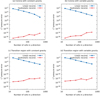 |
Fig. 3. Convergence curves for isothermal and linearly variable temperature hydrostatic equilibrium conditions with constant and variable gravity for the atmospheric data of Table 1. The blue line with circles shows the L1-norm of the pressure error for the standard second order MUSCL-Hancock scheme (linear reconstruction), and the red line with crosses corresponds to the MUSCL-Hancock scheme with local hydrostatic reconstruction. |
In the following test we evaluate the ability of the scheme to manage hydrostatic equilibrium conditions with arbitrary temperature distribution. We expect the local hydrostatic reconstruction scheme to be able to improve the performance of the standard MUSCL-Hancock scheme specially when a low grid resolution in the gravity direction is used. For the analysis we consider the “complete” solar atmosphere, i.e., a cold chromosphere, an abrupt temperature change in the narrow transition region, and a hot corona, with the temperature distribution proposed by Vernazza et al. (1981) as follows:
 (63)
(63)
where the parameters a0, a1, a2, and a3 are chosen according to the temperature values imposed in each layer and the wide and position required for the transition region inside the domain. In this simulation we take a0 = 4.9 × 10⁵ K, a1 = 2 × 108 cm, a2 = 0.5 × 108 cm, and a3 = 5. × 105 K. In Fig. 4 the temperature profile obtained for these values and the consequent hydrostatic pressure distribution are shown, for ρ0 = 10−11 g cm−3 at the base domain, constant gravity g = 2.74 × 104 cm s2, specific heat ratio γ = 5/3, and particular gas constant R = 16.6289196 × 10⁷ erg (K mol)−1 (totally ionized hydrogen).
The numerical results of the hydrostatic condition shown in Fig. 4 are presented in Fig. 5, where the convergence curves for both the linear and the local hydrostatic reconstruction MUSCL-Hancock schemes are plotted. As expected, the results of the scheme with linear reconstruction exhibit the aforementioned third order superconvergence but they present strong errors in the hydrostatic equilibrium preservation when low resolution grids are used. On the other hand, the results corresponding to the local hydrostatic reconstruction technique show a similar convergence rate for large numbers of cells (M ≳ 100), but with smaller errors than the standard scheme, which can be even several orders of magnitude smaller when coarse grids are used. This behavior shows the potential of the local hydrostatic reconstruction scheme, since it allows for improvement of the results for very stratified atmospheres with large temperature gradients, as found in many solar astrophysical applications.
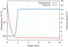 |
Fig. 4. Temperature distribution and hydrostatic pressure profile in the solar atmosphere model by Vernazza et al. (1981) given in Eq. (63). |
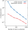 |
Fig. 5. Convergence curves for the numerical results of the hydrostatic equilibrium atmosphere shown in Fig. 4. The blue line with circles shows the L1-norm of the pressure error for the standard second order MUSCL-Hancock scheme (linear reconstruction), and the red line with crosses corresponds to the MUSCL-Hancock scheme with local hydrostatic reconstruction. |
6.2. Diffusion analysis
In this analysis we simply study the ability of the local hydrostatic reconstruction scheme to capture a shock wave traveling in a gravitationally stratified medium. The aim of the analysis is to verify that this scheme does not introduce an excessive numerical diffusion compared to the scheme with linear reconstruction to model the shock wave. In addition, we check the behavior of the hydrostatic scheme in the default AMR module of FLASH, which uses the PARAMESH2 package (MacNeice et al. 2000). This toolkit builds a hierarchy of sub-grids blocks with identical logical structure that cover the physical domain with different resolution levels according to the gradient magnitude of the set refinement variables. Each block is treated as an independent uniform grid, so that the local hydrostatic reconstruction is directly applied on adaptive meshes without the need to modify any subroutine.
For this simulation we consider a blast generated by a pressure pulse located in the solar corona, assuming a linearized temperature distribution for each atmospheric layer given by
 (64)
(64)
We also consider a totally ionized hydrogen atmosphere with variable gravity (see the data on the epigraph of Table 1). The pressure pulse radius is rp = 1 Mm, which is located at the center of the domain in the x-direction and at height hp = 6.5 Mm. Inside the pulse the pressure is 100 times greater than the local hydrostatic pressure and the temperature remains the same as in the corona, with which the plasma density varies according to the equation of state. In Fig. 6 the pressure distribution together with the initial adaptive grid used in the simulation are shown. The strong refinement on the bottom part of the physical domain is due to the presence of the transition region that links the “cold” chromosphere with the “hot” corona. The temperature increases by two orders of magnitude in a relatively thin layer.
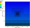 |
Fig. 6. Pressure distribution for the blast model in the solar corona together with the initial adaptive grid for the temperature distribution of Eq. (64). |
Naturally, the numerical results of this configuration must represent the physics of the problem. In this way, we can anticipate that, in the context of an isothermal medium, an initially circular pressure pulse expands radially producing a circular shock wave when it is strong enough. The local hydrostatic reconstruction scheme would be able to capture the circular shape of the shock wave provided that the contribution of the transverse flux in x-direction was correctly implemented. On the contrary, the shock wave travels at different speeds in each direction, causing the wave to lose the expected circular shape. In addition to this result, the hydrostatic numerical code should capture the sharpness of the shock wave with a similar level of numerical diffusion as the conventional linear reconstructed scheme, since an excessive artificial viscosity could mask physical behaviors in very energetic processes.
In Fig. 7 we show the numerical results obtained for both the standard USM solver of the FLASH code with linear reconstruction and the same solver with the local hydrostatic reconstruction implementation. These results correspond to a time of 40 s, where it is assumed that the shock wave has advanced a significant distance but is still strong enough to maintain the steepness that we want to capture. We note in the 2D color plots that the pressure distribution for both schemes (linearly and hydrostatically reconstructed) reproduce the circular shape of the shock wave. Also, we can see in the pressure profile for a vertical centered line that both schemes capture the shock and the posterior expansion inside the pulse in a very similar way. However, the hydrostatically reconstructed scheme is superior to the linearly reconstructed scheme in preserving the hydrostatic equilibrium of the background medium; this can be seen when comparing the maximum and minimum pressure values in the 2D color plots of Fig. 7 (see the highest and the lowest values in the color bars). These differences are due to the increment in the background hydrostatic pressure numerically generated by the standard scheme, which induces a spurious flux from the chromosphere to the corona that raises the pressure. This is an important aspect to take into account when studying the effect of blasts or other events on the chromosphere, for example, in the analysis of possible mechanisms for the formation of Moreton waves, since a nonphysical flux in the chromosphere region could interfere with the sought results. To finish this analysis, we can say that, as expected, the behavior of the hydrostatically reconstructed scheme in adaptive grids does not present any problem.
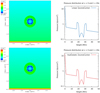 |
Fig. 7. Evolution of a pressure pulse with Δp/p = 100 for t = 40 s. Top panels: standard second order MUSCL-Hancock scheme (linear reconstruction) and bottom panels: same scheme with local hydrostatic reconstruction. |
6.3. Wave-propagation analysis
The last test presented in this work consists in evaluating the ability of the local hydrostatic reconstruction scheme to manage wave propagating solutions. In this case, we are particularly interested in low-amplitude waves propagating in gravitationally stratified atmospheres. For this to occur, forit is crucial to preserve the hydrostatic equilibrium of the background medium because the presence of numerically induced velocities can strongly affect the solution. This topic is of particular interest for helioseismology, where it is sought to study the evolution of low-amplitude waves, driven from the Sun’s interior, which propagate in the solar atmosphere, for example, in the analysis of the photospheric p-modes of sunspots (Kobanov et al. 2008; Jess et al. 2012; Sheeley et al. 2014).
For this analysis we consider the isothermal corona with constant gravity described in Table 1 for which an oscillatory forcing from the bottom boundary is imposed for the velocity component in the y-direction. The forcing is applied on the vertical velocity of the bottom ghost cells such that
 (65)
(65)
where A0 is the wave amplitude, T0 is the oscillation period, and t is the current time. We take T0 = 20 s and three values of amplitude to analyze the numerical results for low (A0 = 1 cm s−1), moderate (A0 = 1000 cm s−1), and high (A0 = 1.5 × 105 cm s−1) amplitudes.
Now, we perform the simulations for different grids with a progressive increasing resolution to evaluate the convergence of the standard and hydrostatically reconstructed schemes, as done in the previous sections, but using for this case of oscillatory velocities the L1-norm of the velocity component in y-direction. Naturally, we do not have a stationary reference solution to carry out the comparison, but we assume that the convergence of the standard second order MUSCL-Hancock scheme is proved, which allows us to use the solution for a very fine grid as a reference solution.
In Fig. 8 we plot the convergence curves with respect to the reference solution corresponding to M = 8192 and t = 200 s for both the standard and hydrostatically reconstructed schemes. We only show the results for low and moderate amplitudes since the curves of each scheme for high-amplitude waves are identical. Observing Fig. 8 we can see the better performance of the local hydrostatic scheme in the modeling of low-amplitude propagating waves, which is entirely due to the well-balanced property of the scheme. Owing to this property, spurious velocities in the gravity direction generated by the standard linear reconstructed scheme do not affect the “stationary part” of the solution. This is clearly observed in Fig. 9 in which we plot the vertical velocity profile in the gravity direction to visualize the “downward movement” of the standard scheme curve with respect to the reference solution. Nevertheless, the convergence curves for moderate-amplitude wave solutions are very similar for both schemes. This similarity is expected since the magnitude of the spurious velocity induced by the standard scheme depends on the atmospheric properties and grid resolution rather than on the wave amplitude, therefore the impact of the spurious velocity on the wave solution tends to be negligible for increasing amplitudes. This is the reason by which the high-amplitude wave solutions present almost identical convergence curves for both schemes. These comments complete the numerical analysis of the local hydrostatic reconstruction scheme.
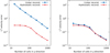 |
Fig. 8. Convergence curves for the wave propagating solution in the corona for t = 200 s and a period T0 = 20 s. Left panel: low-amplitude wave (A0 = 1 cm s−1) and right panel: moderate-amplitude wave (A0 = 1000 cm s−1). The blue line with circles shows the L1-norm of the vertical velocity component error for the standard second order MUSCL-Hancock scheme (linear reconstruction), and the red line with crosses corresponds to the same scheme with local hydrostatic reconstruction. |
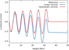 |
Fig. 9. Velocity profile in the gravity direction for the low-amplitude propagating wave in the corona for t = 200 s and a period T0 = 20 s. The reference solution corresponds to the standard second order MUSCL-Hancock scheme with M = 8192 and the other curves were obtained for M = 512. |
7. Conclusions
We performed an analysis of the numerical preservation of the hydrostatic equilibrium of gravitationally stratified atmospheres modeled by Godunov-type schemes with MUSCL-type reconstruction. Firstly, we reviewed the main aspects of standard polynomial reconstruction techniques to show that they are not able to satisfy a hydrostatic equilibrium condition numerically, which makes it necessary to use modified schemes if that condition has to be accomplished. In this way, we proposed a local hydrostatic reconstruction scheme based on the works by Fuchs et al. (2010), Käppeli & Mishra (2016), which assume an ideal gas equation of state to achieve the well-balanced property for hydrostatic equilibrium conditions with constant or linearly variable temperature and constant or variable gravity. We presented several tests through which we verified the numerical behavior of the scheme that was implemented in the USM algorithm of the FLASH code (version 4.5). The numerical results demonstrated the well-balanced property of the local hydrostatic reconstruction technique for the mentioned hydrostatic conditions in ideal gas atmospheres and also proved the better behavior of the scheme in the preservation of the hydrostatic equilibrium with other conditions. We also showed that the local hydrostatic reconstruction technique correctly reproduces discontinuous solutions without introduce excessive artificial viscosity compared to the standard scheme. In addition, the ability of the scheme to manage propagating waves solutions was also verified, showing its superior performance in the treatment of low-amplitude wave propagation problems with respect to the linear reconstructed scheme. We think that these capabilities, together with the relatively simple implementation of the scheme in existing codes based on Godunov with MUSCL reconstruction schemes, make the local hydrostatic reconstruction scheme a good option for the numerical analysis of astrophysical processes that are produced in gravitationally stratified mediums for which the ideal gas equation of state is valid.
The FLASH code is a multiphysics software widely used for astrophysical applications.
PARAMESH is a package of FORTRAN 90 subroutines which provides parallel support with adaptive mesh capability.
References
- Aschwanden, M. J. 2005, Physics of the Solar Corona. An Introduction with Problems and Solutions, 2nd edn. (Berlin: Springer) [Google Scholar]
- Audusse, E., Bouchut, F., Bristeau, M.-D., Klein, R., & Perthame, B. 2004, SIAM J. Numer. Anal., 25, 2050 [Google Scholar]
- Balsara, D. S., & Spicer, D. S. 1999, J. Comput. Phys., 149, 270 [Google Scholar]
- Bell, J. B., Dawson, C. N., & Shubin, G. R. 1988, J. Comput. Phys., 74, 1 [NASA ADS] [CrossRef] [Google Scholar]
- Botta, N., Klein, R., Langenberg, S., & Lützenkirchen, S. 2004, J. Comput. Phys., 196, 539 [NASA ADS] [CrossRef] [Google Scholar]
- Brackbill, J. U., & Barnes, D. C. 1980, J. Comput. Phys., 35, 426 [NASA ADS] [CrossRef] [MathSciNet] [Google Scholar]
- Cargo, P., & Gallice, G. 1997, J. Comput. Phys., 136, 446 [NASA ADS] [CrossRef] [Google Scholar]
- Chen, P. F. 2011, Sol. Phys., 8, 1 [Google Scholar]
- Colella, P., & Woodward, P. R. 1984, J. Comput. Phys., 54, 174 [NASA ADS] [CrossRef] [MathSciNet] [Google Scholar]
- Evans, C. R., & Hawley, J. F. 1988, ApJ, 332, 659 [Google Scholar]
- Felipe, T., Khomenko, E., & Collados, M. 2010, ApJ, 719, 357 [Google Scholar]
- Fjordholm, U. S., Mishra, S., & Tadmor, E. 2011, J. Comput. Phys., 230, 5587 [NASA ADS] [CrossRef] [MathSciNet] [Google Scholar]
- Fryxell, B., Olson, K., Ricker, P., et al. 2000, ApJS, 131, 273 [NASA ADS] [CrossRef] [Google Scholar]
- Fuchs, F. G., McMurry, A. D., Mishra, S., Risebro, N. H., & Waagan, K. 2010, J. Comp. Phys., 229, 4033 [NASA ADS] [CrossRef] [Google Scholar]
- Gardiner, T. A., & Stone, J. M. 2005, J. Comput. Phys., 205, 509 [Google Scholar]
- Gardiner, T. A., & Stone, J. M. 2008, J. Comput. Phys., 227, 4123 [NASA ADS] [CrossRef] [Google Scholar]
- Greenberg, J. M., & Leroux, A. Y. 1996, SIAM J. Numer. Anal., 33, 1 [Google Scholar]
- Gurski, K. 2004, SIAM J. Numer. Anal., 25, 2165 [Google Scholar]
- Jess, D. B., Shelyag, S., Mathioudakis, M., et al. 2012, ApJ, 746, 183 [NASA ADS] [CrossRef] [Google Scholar]
- Käppeli, R., & Mishra, S. 2014, J. Comput. Phys., 259, 199 [NASA ADS] [CrossRef] [Google Scholar]
- Käppeli, R., & Mishra, S. 2016, A&A, 587, A94 [NASA ADS] [CrossRef] [EDP Sciences] [Google Scholar]
- Kobanov, N. I., Kolobov, D. Y., & Chupin, S. A. 2008, Astron. Lett., 34, 133 [NASA ADS] [CrossRef] [Google Scholar]
- Krause, G., Cécere, M., Zurbriggen, E., et al. 2018, MNRAS, 474, 770 [NASA ADS] [CrossRef] [Google Scholar]
- Lee, D., & Deane, A. E. 2009, J. Comput. Phys., 228, 952 [NASA ADS] [CrossRef] [Google Scholar]
- Lee, D., Deane, A. E., & Federrath, C. 2009, in Numerical Modeling of Space Plasma Flows: ASTRONUM-2008, eds. N. V. Pogorelov, E. Audit, P. Colella, & G. P. Zank, ASP Conf. Ser., 406, 243 [NASA ADS] [Google Scholar]
- MacNeice, P., Olson, K. M., Mobarry, C., de Fainchtein, R., & Packer, C. 2000, Comput. Phys. Commun., 126, 330 [NASA ADS] [CrossRef] [Google Scholar]
- Mei, Z., Shen, C., Wu, N., et al. 2012, MNRAS, 425, 2824 [NASA ADS] [CrossRef] [Google Scholar]
- Mignone, A., Bodo, G., Massaglia, S., et al. 2007, ApJS, 170, 228 [Google Scholar]
- Miyoshi, T., & Kusano, K. 2005, J. Comput. Phys., 208, 315 [NASA ADS] [CrossRef] [Google Scholar]
- Miyoshi, T., Terada, N., Matsumoto, Y., et al. 2010, IEEE T. Plasma Sci., 38, 2236 [NASA ADS] [CrossRef] [Google Scholar]
- Murawski, K., Srivastava, A. K., McLaughlin, J. A., & Oliver, R. 2013, Sol. Phys., 283, 383 [NASA ADS] [CrossRef] [Google Scholar]
- Pen, U.-L., Arras, P., & Wong, S. 2003, ApJS, 149, 447 [NASA ADS] [CrossRef] [Google Scholar]
- Powell, K. G. 1994, Approximate Riemann Solver for Magnetohydrodynamics (that Works in More than One Dimension), Tech. Rep. [Google Scholar]
- Powell, K. G., Roe, P. L., Linde, T. J., Gombosi, T. I., & De Zeeuw, D. L. 1999, J. Comput. Phys., 154, 284 [NASA ADS] [CrossRef] [Google Scholar]
- Sheeley, Jr., N. R., Warren, H. P., Lee, J., et al. 2014, ApJ, 797, 131 [NASA ADS] [CrossRef] [Google Scholar]
- Tarr, L. A., Linton, M., & Leake, J. E. 2016, AAS/Solar Physics Division Meeting #47, 101.05 [Google Scholar]
- Toro, E. 2009, Riemann Solvers and Numerical Methods for Fluid Dynamics, 3rd edn. (Berlin: Springer) [Google Scholar]
- Tóth, G. 2000, J. Comput. Phys., 161, 605 [Google Scholar]
- van Leer, B. 1979, J. Comput. Phys., 32, 101 [Google Scholar]
- Vernazza, J. E., Avrett, E. H., & Loeser, R. 1981, ApJS, 45, 635 [NASA ADS] [CrossRef] [Google Scholar]
- Xing, Y., & Shu, C.-W. 2013, J. Sci. Comput., 54, 645 [Google Scholar]
- Zhang, Y., Kitai, R., Narukage, N., et al. 2011, PASJ, 63, 685 [Google Scholar]
- Ziegler, U. 2004, J. Comput. Phys., 196, 393 [NASA ADS] [CrossRef] [Google Scholar]
- Zingale, M., Dursi, L. J., ZuHone, J., et al. 2002, ApJS, 143, 539 [NASA ADS] [CrossRef] [Google Scholar]
All Tables
Simulation data for the solar corona and the transition region of the equilibrium atmosphere background.
All Figures
|
Fig. 1. Definitions for a generic cell i, j in a structured Cartesian grid. |
| In the text | |
|
Fig. 2. First (red lines) and second (blue lines) order standard reconstruction in a hydrostatic pressure distribution. The solid black line represents the equilibrium hydrostatic pressure p0(y). |
| In the text | |
|
Fig. 3. Convergence curves for isothermal and linearly variable temperature hydrostatic equilibrium conditions with constant and variable gravity for the atmospheric data of Table 1. The blue line with circles shows the L1-norm of the pressure error for the standard second order MUSCL-Hancock scheme (linear reconstruction), and the red line with crosses corresponds to the MUSCL-Hancock scheme with local hydrostatic reconstruction. |
| In the text | |
|
Fig. 4. Temperature distribution and hydrostatic pressure profile in the solar atmosphere model by Vernazza et al. (1981) given in Eq. (63). |
| In the text | |
|
Fig. 5. Convergence curves for the numerical results of the hydrostatic equilibrium atmosphere shown in Fig. 4. The blue line with circles shows the L1-norm of the pressure error for the standard second order MUSCL-Hancock scheme (linear reconstruction), and the red line with crosses corresponds to the MUSCL-Hancock scheme with local hydrostatic reconstruction. |
| In the text | |
|
Fig. 6. Pressure distribution for the blast model in the solar corona together with the initial adaptive grid for the temperature distribution of Eq. (64). |
| In the text | |
|
Fig. 7. Evolution of a pressure pulse with Δp/p = 100 for t = 40 s. Top panels: standard second order MUSCL-Hancock scheme (linear reconstruction) and bottom panels: same scheme with local hydrostatic reconstruction. |
| In the text | |
|
Fig. 8. Convergence curves for the wave propagating solution in the corona for t = 200 s and a period T0 = 20 s. Left panel: low-amplitude wave (A0 = 1 cm s−1) and right panel: moderate-amplitude wave (A0 = 1000 cm s−1). The blue line with circles shows the L1-norm of the vertical velocity component error for the standard second order MUSCL-Hancock scheme (linear reconstruction), and the red line with crosses corresponds to the same scheme with local hydrostatic reconstruction. |
| In the text | |
|
Fig. 9. Velocity profile in the gravity direction for the low-amplitude propagating wave in the corona for t = 200 s and a period T0 = 20 s. The reference solution corresponds to the standard second order MUSCL-Hancock scheme with M = 8192 and the other curves were obtained for M = 512. |
| In the text | |
Current usage metrics show cumulative count of Article Views (full-text article views including HTML views, PDF and ePub downloads, according to the available data) and Abstracts Views on Vision4Press platform.
Data correspond to usage on the plateform after 2015. The current usage metrics is available 48-96 hours after online publication and is updated daily on week days.
Initial download of the metrics may take a while.