| Issue |
A&A
Volume 631, November 2019
|
|
|---|---|---|
| Article Number | A149 | |
| Number of page(s) | 28 | |
| Section | Planets and planetary systems | |
| DOI | https://doi.org/10.1051/0004-6361/201936302 | |
| Published online | 13 November 2019 | |
Shape model and spin-state analysis of PHA contact binary (85990) 1999 JV6 from combined radar and optical observations★,★★
1
Centre for Astrophysics and Planetary Science, University of Kent,
Canterbury, UK
e-mail: This email address is being protected from spambots. You need JavaScript enabled to view it.
2
Lunar and Planetary Laboratory, University of Arizona,
Tucson,
Arizona, USA
3
Lunar and Planetary Institute, Universities Space Research Association,
Houston,
Texas, USA
4
Planetary Science Section, Jet Propulsion Laboratory/Caltech,
Pasadena,
California, USA
5
Astrophysics Research Centre, Queens University Belfast,
Belfast, UK
6
Planetary Sciences Institute,
Tucson,
Arizona, USA
7
Planetary and Space Sciences, School of Physical Sciences, The Open University,
Milton Keynes, UK
8
Institute for Astronomy, University of Edinburgh,
Royal Observatory, Edinburgh, UK
9
Arecibo Observatory, University of Central Florida,
Arecibo,
Porto Rico, USA
10
National Radio Astronomy Observatory,
Green Bank,
West Virginia, USA
Received:
12
July
2019
Accepted:
1
October
2019
Abstract
Context. The potentially hazardous asteroid (85990) 1999 JV6 has been a target of previously published thermal-infrared observations and optical photometry. It has been identified as a promising candidate for possible Yarkovsky-O’Keefe-Radzievskii-Paddack (YORP) effect detection.
Aims. The YORP effect is a small thermal-radiation torque considered to be a key factor in spin-state evolution of small Solar System bodies. In order to detect YORP on 1999 JV6 we developed a detailed shape model and analysed the spin-state using both optical and radar observations.
Methods. For 1999 JV6, we collected optical photometry between 2007 and 2016. Additionally, we obtained radar echo-power spectra and imaging observations with Arecibo and Goldstone planetary radar facilities in 2015, 2016, and 2017. We combined our data with published optical photometry to develop a robust physical model.
Results. We determine that the rotation pole resides at negative latitudes in an area with a 5° radius close to the south ecliptic pole. The refined sidereal rotation period is 6.536787 ± 0.000007 h. The radar images are best reproduced with a bilobed shape model. Both lobes of 1999 JV6 can be represented as oblate ellipsoids with a smaller, more spherical component resting at the end of a larger, more elongated component. While contact binaries appear to be abundant in the near-Earth population, there are only a few published shape models for asteroids in this particular configuration. By combining the radar-derived shape model with optical light curves we determine a constant-period solution that fits all available data well. Using light-curve data alone we determine an upper limit for YORP of 8.5 × 10⁻⁸ rad day−2.
Conclusions. The bifurcated shape of 1999 JV6 might be a result of two ellipsoidal components gently merging with each other, or a deformation of a rubble pile with a weak-tensile-strength core due to spin-up. The physical model of 1999 JV6 presented here will enable future studies of contact binary asteroid formation and evolution.
Key words: minor planets, asteroids: individual: (85990) 1999 JV6 / methods: observational / methods: data analysis / techniques: photometric / techniques: radar astronomy / radiation mechanisms: thermal
Table A.2 is only available at the CDS via anonymous ftp to cdsarc.u-strasbg.fr (130.79.128.5) or via http://cdsarc.u-strasbg.fr/viz-bin/cat/J/A+A/631/A149
Based in part on observations collected at the European Organisation for Astronomical Research in the Southern Hemisphere under ESO programme 185.C-1033(R) and the Arecibo Planetary Radar observations collected under programmes R2959, R3035 and R3036.
© ESO 2019
1 Introduction
The Yarkovsky-O’Keefe-Radzievskii-Paddack (YORP) effect is a small torque due to the reflection, absorption, and thermal re-emission of sunlight from an asteroid surface (Rubincam 2000). The effect is strongest for small (metre- to kilometre-sized) bodies close to the Sun, specifically the near-Earth asteroids (NEAs). The YORP effect can alter the rotational momentum of NEAs, that is the spin-axis obliquity and rotation period. Acting on timescales shorter than collisions (Vokrouhlický et al. 2003), it is now considered to be the main driving factor in the spin-state evolution of small Solar System bodies. The Yarkovsky effect, a sister effect that alters total angular momentum and energy, for instance introducing a secular trend in the evolution of the semi-major axis, is sensitive to the obliquity of the target. The coupling between the YORP and Yarkovsky effects plays a crucial role in the delivery of small bodies into the near-Earth region, and can significantly affect orbital predictions for potentially hazardous asteroids (PHAs, Rubincam 2000; Bottke et al. 2002; Chesley et al. 2003). The rotation-rate aspect of the YORP effect has wide implications, with the YORP-induced spin-up leading to re-arrangement of surface material and formation of characteristic “spinning-top” or “YORPoid” shapes (Ostro et al. 2006; Scheeres et al. 2006), or the formation of binary asteroids by driving the bodies to their rotational fission limit (Walsh et al. 2008, 2012). Another manifestation of thermal torques, referred to as “binary YORP” (B-YORP), affects the evolution of mutual orbits of components in asteroid binary systems, causing them to either separate or collapse to form contact binaries, but has yet to be confirmed experimentally (Ćuk & Burns 2005).
To date, the YORP-induced period change has been confirmed for only seven NEAs: (54509) YORP (Lowry et al. 2007; Taylor et al. 2007), (1862) Apollo (Kaasalainen et al. 2007), (1620) Geographos (Ďurech et al. 2008), (3103) Eger (Ďurech et al. 2012), (25143) Itokawa (Lowry et al. 2014), (161989) Cacus (Ďurech et al. 2018), and (101955) Bennu (Nolan et al. 2019). Notably, all of those detections are YORP-induced rotational spin-ups, while the YORP theory predicts rotational slow-down as well; for example Rozitis & Green (2013). One proposed explanation for the prevalence of observed YORP-induced spin-ups is the so-called “tangential YORP”, an effect that comes from thermal re-emission of radiation absorbed by boulders that produces a recoil tangential to the surface of the asteroid (Golubov et al. 2014).
In order to provide new observational evidence for the development of YORP theory, we established an ongoing observing campaign tocharacterise selected NEAs, which started with a European Southern Observatory Large Programme (ESO LP) observing campaign. Since 2010 we have been using the ESO New Technology Telescope (NTT) and the ESO Faint Object Spectrograph and Camera v.2 (EFOSC2, Buzzoni et al. 1984) instrument at the La Silla Observatoryin Chile for optical light-curve and spectroscopic observations of NEAs. We also observed selected targets in the mid-infrared using the ESO Very Large Telescope (VLT) and the VLT Imager and Spectrometer for mid Infrared instrument (Lagage et al. 2004) at the Paranal Observatory in Chile and the Spitzer Space Telescope. While the bulk of the ESO LP observations is complete, the campaign continues, collecting optical photometry with a range of small-to-medium-sized telescopes. The optical and thermal infrared observations are supplemented by radar data for some targets. We combine the observational data to develop shapes, spin-states, and physical properties, and develop YORP torque models using the Advanced Thermophysical Model (Rozitis & Green 2011, 2012, 2013).
The PHA (85990) 1999 JV6 (hereafter referred to as JV6) is an Apollo group asteroid discovered on 13 May 1999 by the Massachusetts Institute of Technology Lincoln Laboratory’s Near-Earth Asteroid Research program (Stokes et al. 2000). It has been identified as spectral type Xk (Binzel et al. 2001) by the Small Main-Belt Asteroid Spectroscopic Survey (SMASS) taxonomic survey (Bus 1999; Bus & Binzel 2002). Thermal infrared observations from the ExploreNEOs near infrared survey with the Spitzer Space Telescope (Trilling et al. 2010) were used to estimate the diameter of the object to be  , with a low albedo of
  (Mueller et al. 2011). The JV6 was also the target of the Wide-field Infrared Survey Explorer (WISE) spacecraft observations, resulting in a diameter measurement of 451 ± 26 m, and an optical albedo of 0.095 ± 0.023 (Mainzer et al. 2011). Optical observations from January 2014 at the Palmer Divide Station demonstrated a high light-curve amplitude of 0.87 mag, with a synodic rotation period of 6.538 ± 0.001 h (Warner 2014). The object was also observed at the Palmer Divide Station in January 2015 when the light-curve amplitude was slightly higher, 0.93 mag, and the synodic rotation period was 6.543 ± 0.002 h (Warner 2015).
We monitored JV6 photometrically as one of our ESO LP targets at the NTT in 2013. We collected additional light-curve data with associated programmes at the 0.6 m Table Mountain Observatory (TMO) telescope in California (USA) in 2015, and at the 2.5 m Isaac Newton Telescope (INT) in La Palma (Spain) in 2007, 2008, and 2016. Close approaches to Earth in 2015, 2016, and 2017 offered an opportunity to observe JV6 with ground-based radar facilities. We observed JV6 as the target of a dedicated Arecibo planetary radar campaign in January 2015, 2016, and 2017. We also followed the object with the Goldstone Solar System Radar (GSSR) in January 2016, with part of the observations performed in bistatic mode with the Green Bank Telescope (GBT) in West Virginia (USA).
A comprehensive description of our observing campaign for JV6 including optical photometry, radar spectra, and radar imaging is contained in Sect. 2. We combined and analysed the observational data to obtain a detailed shape model of JV6. The results of rotational pole determination and shape modelling are discussed in Sect. 3. The result of light-curve-only analysis providing a determination of an upper limit of the YORP strength, as well as spin-state analysis that uses all available light curves and the best radar-derived model, are presented in Sect. 4.
2 Observations of (85990) 1999 JV6
2.1 Optical light-curve observations
The optical light-curve data for JV6 span ten years. The orbit of this PHA is inclined at only ~ 5° to the ecliptic and has a semi-major axis of ~1.008 AU. Thus, the object regularly appears in a very constrained location in the sky, with a slowly changing range of observer-centred ecliptic latitudes and longitudes (see Fig. 1). The orbital configuration makes JV6 a convenient target for continued monitoring. A summary of all available light curves, including an overview of observing circumstances, distance from Earth and the Sun, and the phase angle at which the target was observed is listed in Table 1. The observing geometries for different types of observations used here are illustrated in Fig. 1.
The observing strategy for obtaining the photometric light curves is to keep the asteroid image in each frame from trailing by providing non-sidereal tracking on the moving target. If sidereal tracking is necessary, it is preferred to keep the exposure time short enough so that the full width at half maximum (FWHM) of the profile of the image of the asteroid is below the seeing conditions. The target brightness can then be measured using a circular aperture with radius usually around two to three FWHMs of the profile of the asteroid. In instances where the short tracking times resulted in a low signal-to-noise ratio (S/N) on the asteroid image, we co-added multiple frames and performed aperture photometry on the resulting image. The brightness of the target was then compared to the average brightness of the background stars and the relative light curve was extracted. The light curves obtained in our ESO LP programme are labelled with IDs 1–9 and 23–28 in Table 1, and are presented in panels marked with those IDs in Figs. A.1 and A.4. The light-curve data can be accessed in Table A.2, available at the CDS.
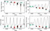 |
Fig. 1 Asteroid (85990) 1999 JV6 observing geometries during the optical and radar observations. The graphs display different quantities as a function of time. Top two panels: positions of the object in the ecliptic coordinate system, latitude and longitude, as observed from Earth. Bottom two panels: phase angle, the angle between the positions of the Earth and Sun as observed from the target, and geocentric distance to the target. Optical light curve data from the NTT are marked with filled black circles, with light-curve data from supporting campaigns marked with filled green circles. Red squares represent the published light-curve data. The black cross symbols mark when the Arecibo radar data were collected, and the red crosses mark Goldstone observations. The black continuous line represents the ephemeris of the object. The break in the Y -axis in all four graphs indicates the gap between June 2008 and July 2012. |
2.1.1 New Technology Telescope – 2013
The JV6 was one of our optical photometry targets at the ESO 3.6 m NTT telescope in La Silla (Chile), using the EFOSC2. The charge-coupled device (CCD) detector of EFOSC2 has 2048 × 2048 pixels and a field of view of 4.1′ × 4.1′. We performed the observations of JV6 in imaging mode using 2 × 2 binning on the detector, and with the Bessel V filter. We detected JV6 at the NTT on three nights, between 4 and 6 February 2013 (ESO programme 185.C-1033(R)). Strong winds imposed pointing restrictions for the telescope and forced a break in the observing, which resulted in obtaining two separate light-curve segments on 4 February. We collected two additional partial light curves on 5 and 6 February, but due to their low S/N they are not included in the analysis. The data were reduced using the standard CCD reduction procedures. Before performing the photometric measurements, we co-added the individual frames in groups of three to improve the S/N of the resulting light curve.
2.1.2 Isaac Newton Telescope – 2007, 2008 and 2016
We monitored asteroid JV6 with the 2.5 m INT in La Palma (Spain) using the Wide-Field Camera (WFC). The WFC is an array of four CCD chips of 2048 × 4100 pixels each, with a total field of view of 34′ × 34′. The JV6 observations were performed using Gunn r filter in 2007 and 2008, and Harris V filter in 2016. We observed the target on four different nights in 2007, three in 2008, and another four in 2016 (programme IDs I/2007A/4 and I/2016A/10), giving a total of ten light-curve data sets. The data were reduced using standard CCD reduction procedures.
2.1.3 Table Mountain Observatory – 2015
Between 23 and 25 January 2015, we observed JV6 with the Jet Propulsion Laboratory’s TMO’s 0.6 m telescope in California (USA). The telescope is equipped with a 1024 × 1024 pixel CCD camera with an 8.9′ × 8.9′ field of view. The JV6 imaging sequence was collected using the R filter. The data-reduction process required standard CCD reduction steps. Three light curves covering just over one full rotation each were obtained.
2.1.4 Published data
The analysis presented here also includes previously published photometry obtained at the Palmer Divide Station (Warner 2014, 2015). The processed light curves were retrieved from the Asteroid Light-curve Data Exchange Format (ALCDEF) database (Warner et al. 2011). Those light curves are labelled with IDs 10–22 in Table 1.
2.1.5 Light-curve data selection for shape and spin-state modelling
The collected light curves have peak-to-peak amplitudes between 0.75 and 1.44 mag with two sharp minima, consistent with other contact binary NEAs; for example Itokawa (Lowry et al. 2014). The data are plotted with red dots in Figs. A.1 and A.4. We selected light curves with the highest S/N for the convex inversion. Two light curves from 2007 were used (IDs 1 and 4 in Table 1), and the 2008 set was limited to the only full light curve (ID 7). These, combined with selected light curves from 2013–2016 (IDs 8–23 and 26–28), gives a total of 22 light curves included in the light-curve-only pole scan.
We limited the light-curve data included in the radar shape modelling to a subset of light curves obtained closest to the radar runs. Including light-curve data in radar shape modelling provides improved constraint on the spin state. However, it is useful to have a shape model independent of the light curves when performing the spin-state analysis described in Sect. 4.2. We therefore limited the light-curve dataset to ensure that the model is independent from optical light-curve observations taken at other epochs; in other words light curves excluded from the shape model analysis were reserved for the search for YORP. For the combined fit we used the light curves with IDs 19–21 (Warner 2015), 23 (from TMO, 2015), and 26–27 (from INT, 2016); see Table 1 for the numerical IDs of all the light curves. For computational efficiency during the combined radar and optical data fit we binned the light curves with a resolution of 15° in rotation phase, averaging the asteroid relative brightness in each bin.
2.2 Planetary radar observations
The radar observations of Solar System bodies are performed mainly at the Arecibo (Puerto Rico, USA) and Goldstone (California, USA) facilities. The radar images can be highly detailed, providing information about small surface features, like boulders and craters, with spatial resolution down to the level of 3.75 m possible for some high-S/N targets (a resolution of 7.5 m was achieved for JV6) and large concavities can be easily modelled with the radar data. Even when high-resolution imaging with a radar is not possible, combining radar and light-curve observations can improve shape determination, or, at the very least, help to constrain the rotation pole (Ostro et al. 2002). Moreover, using a pre-determined radar shape model to derive artificial light curves greatly simplifies the spin-state analysis performed when attempting to detect YORP (Lowry et al. 2007; Taylor et al. 2007).
Two types of radar data were collected for JV6. Disk-integrated data, called continuous-wave, or cw echo power spectra, and delay-Doppler imaging data. The cw spectra contain no information about the delay of the radar signal reflected off different locations on the asteroid surface. Due to the Doppler shift of the signal caused by the rotation of the asteroid the returning echo covers a range of frequencies and the cw represents a power spectrum of the echo. The bandwidth of the echo gives an indication of the object size when the pole orientation and rotational period are known (Ostro et al. 2002). For JV6, due to bifurcation of the target, we also see occasional drops in the signal power within the spectrum; see Figs. A.3–A.5. For the purpose of the shape modelling we masked the cw spectra to show only the outer edges of the echo, so that the bandwidth information can be clearly decoded, and to leave out the high S/N “spikes” that would dominate the χ2 calculations in the fit and could lead to unrealistic shape determination. Where possible, two masks were applied, so that the bandwidths of both components could be indicated. Any signal outside the masked region was given zero weight.
The continuous waveform of the radio signal emitted for the purpose of radar imaging is modulated with a pseudo-random code. This can be achieved in two ways, namely by modulation of either signal phase or frequency. The first technique, called binary phase code, was used for most radar imaging observations presented here, both at Arecibo Observatory and with the GSSR (Table 2). The frequency-modulated, or “chirped”, observing mode was used for the bistatic observations on 9 January with Goldstone transmitting and the GBT receiving. The received signal is correlated against the modulation pattern, providing information about the distance between theobserver and the parts of the surface of the target that reflect the signal. The delay resolution of radar images is usually expressed in baud-length, which is the time resolution of the signal modulation. Additionally, the Doppler shift of the returning signal is measured, adding a second dimension to the radar image (Ostro et al. 2002).
The radar imaging frames scan a wide range of frequencies and possible delays, with only a small area in the raw images containing signal from the asteroid. In order to increase computational efficiency and speed up the fitting procedure, we masked the imaging frames, to include as little background as possible. We set up the initial masks manually by defining rectangular regions that roughly contain the signal. After establishing an initial model, we generated synthetic radar images that were used to set up more accurate masks, to be used during the refinement of the model. For any image, the mask would cover the area of the image where the radar signal is expected to be, plus an extra five pixels (following Magri et al. 2011). Pixel values outside the mask were given zero weight.
A chronological list of optical light curves of asteroid (85990) 1999 JV6 used in this study.
2.2.1 Arecibo – 2015, 2016 and 2017
The William E. Gordon telescope in Arecibo, Puerto Rico (USA), is a 305 m fixed-dish radio telescope equipped with an S-band (2380 MHz) planetary radar transmitter. We observed JV6 with Arecibo on five nights between 14 and 18 January 2015, and for a few additional hours on 28 January 2015. The radar echo power cw spectra were taken on each night, as well as imaging, mainly with 0.2 μs (~ 30 m) baud-length code. During the time it was observed in 2015, the object had made an approach to Earth at ~ 0.092 AU and was slowly receding.
We observed JV6 again when it was as close to Earth as 0.053 AU in January 2016 with the Arecibo planetary radar on a further five nights: 13, 14, 16, 17, and 18 January 2016. The approach in 2016 was closer than in 2015, meaning that higher-resolution imaging was possible, with 0.05 μs (7.5 m) baud-lengthobservations on one night, and the bulk of the imaging performed with 0.1 μs (15 m) baud-length code signal. We revisited JV6 with Arecibo on 14 and 15 January 2017 when it was at about 0.082 AU from Earth, obtaining a series of 0.2 μs (30 m) baud-length images. A summary of the Arecibo observations is presented in Table 2.
2.2.2 Goldstone and Green Bank – 2016
We also observed JV6 with the GSSR facility. Its fully steerable DSS-14 70 m antenna is a part of the Goldstone Deep Space Networkcomplex in the Mojave Desert, California, USA. DSS-14 is equipped with an X-band transmitter with a nominal signal frequency of 8560 MHz. We performed the GSSR observations of JV6 in both monostatic and bistatic mode. In monostatic mode the GSSR was used for both transmitting and receiving the signal. In bistatic mode the system used the Robert C. Byrd GBT for recording the returning signal. The GBT is a steerable 100 m antenna, located in West Virginia, USA.
We targeted JV6 with GSSR between 8 and 13 January 2016 obtaining cw spectra and high-resolution delay-Doppler images. The closest approach during the GSSR run was to ~ 0.035 AU. The range resolution obtained was down to 0.125 μs (18.7 m) for observations in monostatic mode, and 0.05 μs (7.5 m) for bistatic observations. A summary of the Goldstone observations is presented in Table 2.
2.2.3 Radar data selection for modelling
Our radar shape modelling of JV6 initially concentrates on the highest-resolution imaging and cw spectra that provide additional geometry information at a low computational cost of including them in the fit. For the combined light curve and radar pole search we selected the cw spectra to be representative of the observing campaign, and to cover the full range of rotation phases. A total of eight cw spectra from Arecibo were used, four from each year. The final refined combined radar and light-curve shape modelling included all available cw observations. The radar power spectra are shown in Figs. A.3–A.6, and descriptions of the spectra are gathered in Table A.1.
When selecting the radar images for a pole search the main criteria were the rotational phase coverage and sky coverage. Ensuring an even distribution of rotational phases and as broad a range of observational geometries as possible translates to an optimal coverage of the surface of the asteroid being imaged with radar. We focused on the 0.1 μs (15 m) and 0.2 μs (30 m)-baud imaging from Arecibo, as well as the baud-lengths 0.05 μs (7.5 m) and 0.125 μs (18.7 m) from Goldstone. At the initial phase of the shape modelling we included a few frames with a baud-length of 0.25 μs (37.5 m) from Goldstone. Using low-resolution images provides additional geometry information and has the advantage of computational efficiency when it comes to comparison between synthetic echoes and observations over the high-resolution imaging. We dropped these lowest-resolution frames at a more advanced stage of the shape modelling, when the shape details became a priority. The observation set used for the refined combined radar and light-curve shape modelling included all frames with 0.2 μs (30 m), 0.1 μs (15 m), and 0.05 μs (7.5 m) baud-length from Arecibo, and 0.125 μs (18.7 m) and 0.05 μs (7.5 m) from Goldstone. All of the imaging frames used in the pole search and the detailed shape modelling are listed in Table A.1, and the images are shown in Figs. A.11–A.24.
3 Shape and spin-state modelling
3.1 Pole search with light-curve data – convex inversion results
The shape fitting with radar data is an iterative process that is highly sensitive to the initial conditions, requiring a first estimate of some of the model parameters. Having a pre-determined rotation pole and sidereal period solution can increase the efficiency of the fitting procedure. Thus, to first constrain the pole and period, we concentrated on light-curve data only, using an approach based on convex light-curve inversion methods (Kaasalainen & Torppa 2001; Kaasalainen et al. 2001; Ďurech et al. 2010). Light-curve inversion methods are powerful tools for recovering shape models of small Solar System bodies. Light-curve inversion models can successfully reproduce even small-scale light-curve features even though what can be reliably modelled is usually only a convex hull of the real object. Breaking the inherent degeneracy resulting from introducing more realistic features, like bifurcation or craters, to the model requires including another source of shape information in the modelling process.
We set up a grid of possible pole positions, with a 5° × 5° resolution expressed in ecliptic coordinates, that is ecliptic longitude λ and ecliptic latitude β, covering theentire celestial sphere. At each grid point, the shape and sidereal rotation period were optimised to best reproduce the light-curve data (Kaasalainen & Torppa 2001). We assume the principal axis rotation, so the Z-axis of the bodyis aligned with the spin vector and the axis of maximum inertia, but the X-axis of the bodydoes not need to overlap with the minimum inertia axis. Thus, the X-axis was selected within the body such that it would be in the plane of the sky at T0, and during the fitting T0 was held fixed. It was arbitrarily selected to be at the beginning of the first light curve in the available set (2 March 2007).
The results of the pole search under the assumption of a constant sidereal rotation period are presented in Fig. 2. The position of the rotation pole is generally constrained to the southern ecliptic hemisphere by this initial search. The shape models with χ2 not exceeding 10% above the minimum value cover the celestial sphere almost up to ecliptic latitude − 40° with χ2 values decreasing closer to the south ecliptic pole. There are two main factors as to why the pole ecliptic longitude cannot be well constrained for JV6. Firstly,there are limited observing geometries available, with the ecliptic latitude at which JV6 was observed varying only between − 6.8° and 14.5° and phase angle between 7.8° and 34.1° (the observing conditions are listed in Table 1). Secondly, the pole happens to be located at low ecliptic latitudes, so absolute angular distances between poles at different ecliptic longitudes are much shorter than in the vicinity of ecliptic plane, making similar possible solutions less distinguishable. The best-fit light-curve-inversion model we obtained has the pole located at λ = 55°, β = −75°, with the 1σ uncertainty great circle of 15°-radius; the parameters are summed up in Table 3.
The shape derived for the best-fit pole is illustrated in Fig. 3. As a result of trying to represent a strongly non-convex body, the best-fit convex shape model features large planar surfaces. Those replace the obvious concavities that are apparent in the radar imaging, but not seen in the synthetic radar images produced using the convex model, as presented in Fig. 4. The large flat surface elements ensure a good fit to the light-curve data; see example in Fig. 5. Synthetic light curves generated for all available data (presented in Table A.2) are shown in Fig. A.1.
Radar observations of asteroid (85990) 1999 JV6.
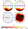 |
Fig. 2 Results of the convex light-curve inversion pole search for asteroid (85990) 1999 JV6, projected on the celestial sphere described in ecliptic coordinates. The blue line marks the ecliptic plane with latitude β = 0°, with some additional circles of latitude marked with black lines and labelled with blue numerals. The red line marks longitude λ = 0° and the green line λ = 180°, with selected meridians marked with black lines and labelled with red numerals. From top-left clockwise, the projections show the eastern (E), western (W), southern (S), and northern (N) hemispheres of the sky, with coordinates of the central point in each projection being (λ = 90 °, β = 0°), (λ = 270 °, β = 0°), (β = −90 °), and (β = +90°). The colour changes from black at the minimum χ2 through red to yellow for higher values of χ2, and the white region represents all the solutions with χ2 more than 50% above the minimum χ2. |
Summary of spin-state parameters for (85990) 1999 JV6 from light-curve inversion and radar-based approaches.
3.2 Pole search with the radar data – two-ellipsoid model
Modelling radar data, which we performed here using the SHAPE modelling software (Hudson 1994; Magri et al. 2007), requires an initial informed guess about the shape model at the beginning of the process. The shape is later refined by introducing increasing surface details. The convex light-curve inversion model fails to fit the radar echoes that show clear bifurcation of the shape, as shown in an example in Fig. 4. Therefore, rather than using the convex-inversion model as an initial condition for the SHAPE modelling software, we manually set up the initial shape. Since the object echoes resembled those of other contact binary asteroids, for example (8567) 1996 HW1 (Magri et al. 2011), a two-ellipsoid model was adopted.
The shape model is represented with two ellipsoidal components, each described by three axial lengths as well as three positional and three angular parameters that can be optimised. Each ellipsoidal component can be rotated in any direction, with Euler anglesused to describe the orientation. The first Euler angle is used to rotate the ellipsoidal component around its Z-axis, then the second angle is used to rotate the body around the new X′ -axis, and finally the third to rotate around the now-rotated Z′-axis. Both components are set in an arbitrary common coordinate system, which is later used as the body-fixed coordinate system. The X, Y, and Z coordinates of the centre for each component can be adjusted. The parameters of the rough two-ellipsoid model were set up by visually matching the synthetic echoes output by SHAPE to a few imaging frames with the highest resolution. The best-fit period and an arbitrarily selected pole, located close to the best-fit pole from the convex light-curve inversion pole search, were used to generate the synthetic echoes. We made manual adjustments until the fit to the radar echoes was satisfactory. The two-ellipsoid shape obtained this way was used as an initial approximation for further study.
In a new pole search, performed using a combination of the selected radar and light-curve data, the two-ellipsoid shape model was optimised together with the sidereal rotation period at a range of possible pole positions. To acquire a full picture we performed the pole search on a coarse grid. The pole positions were selected to be approximately evenly distributed on the celestial sphere with a 10° separation in ecliptic latitude (β), and 10° angular separation as calculated along circles of constant latitude. However, as we established using the convex light-curve inversion of available light curves, the rotation pole could be constrained to negative latitudes. Therefore, we focused on only the southern ecliptic latitudes, running the optimisation also on a finer rectangular grid with a 4° separation in λ and 2° in β. The region enclosed pole positions with λ from 0° to 356° and β from − 90° to − 60° (15° away from the best-fit pole). The χ2 value that reflected the quality of the fit was recorded for each grid point. To calculate the χ2 we compare the radar data with synthetic spectra and images generated assuming cosine scattering law. Figure 6 shows the result of the two-ellipsoid pole search projected onto the celestial sphere.
We better constrain the pole position by combining radar and light-curve data than when using the light curves alone. The uncertainty region (with χ2 values raising by no more than 10% above the minimum) is roughly circular and close to the southern ecliptic pole, with a radius ≈ 5°. The best pole solution from the two-ellipsoid radar search is located at λ = 144°, β = −84°, and the corresponding shape is shown in Fig. 7. The refined sidereal rotation period for the two-ellipsoid model is 6.536783 ± 0.000007 h. We analysed the sizes of both ellipsoidal components for the best shape models produced during the pole search, having the χ2 quality-of-fit value not more than 10% above the minimum value, in order to assess the dimensions and spatial orientations of both lobes. The listed uncertainties are based on the standard deviation of the values obtained for the analysed models. We determine that both lobes are prolate ellipsoids, with the smaller lobe having axial lengths of (346 ± 15) m, (279 ± 8) m, and (291 ± 13) m. The Euler angles to rotate the smaller component are 23° ± 18°, − 21° ± 50°, and 20° ± 25°. The larger lobe is more elongated, with axial lengths of (582 ± 17), (322 ± 7), and (331 ± 9) m. The Euler angles to rotate the larger component are − 9° ± 2°, − 26° ± 14°, and − 3° ± 2°, and therefore the orientation of the larger lobe is better constrained relative to the common reference frame. The centres of both components are separated by (270 ± 14) m along the X-axis, (24 ± 4) m along the Y-axis, and (6 ± 5) m along the Z-axis. The smaller ellipsoid sits close to the end of the larger component in a configuration similar to (25143) Itokawa (Demura et al. 2006), albeit with both components lying in the X–Y plane, also resembling (8567) 1996 HW1, but with less prominent neck region (Magri et al. 2011).
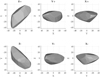 |
Fig. 3 Best-fit convex shape model of (85990) 1999 JV6. The model was produced as a result of a pole search using light-curve data only, assuming a zero-YORP (constant period) solution, and has the pole located at λ = 55°, β = − 75°. Top row (leftto right): views along the Z, Y and X axes of the body-centric coordinate frame from the positive end of the axis. Bottom row (left to right): views along the Z, Y and X axes from their negative ends. For the model to be physically feasible under the assumption of principal-axis rotation, the Z-axis of the body (also the spin axis) should be aligned with the shortest axis of inertia. There is no relation between the longest axis of inertia and the X-axis of the body, instead the X-axis is arbitrarilyselected so that it would be in the plane of the sky at T0. The units onthe X, Y, and Z axes are arbitrary, as the light-curve convex inversion model is not scaled in size. |
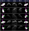 |
Fig. 4 Comparison of fits of the convex-light-curve-inversion and best-fit radar shape models of asteroid (85990) 1999 JV6 to an example subset of the radar imaging data (the model is summarised in Table 3). Each five-image subpanel is made of: plane-of-sky projection of the convex-light-curve-inversion model (sky 1), the synthetic echo generated using the convex model (fit 1), the observational data (data), echo simulated from the radar best-fit model (fit 2), and plane-of-sky projection of the radar best-fit model (sky 2). The convex model was scaled to have approximately the same volume as the radar model. While the convex-light-curve-inversion model reproduces the light-curve data fairly well (which are fully illustrated in Fig. A.1) and even some general shape properties seen in the radar echoes it fails to reproduce the obvious bifurcation of JV6. On the data and synthetic-echo images the delay increases downwards and the frequency (Doppler) to the right. The plane-of-sky images are orientated with celestial north (in equatorial coordinate system) to the top and east to the left. The principal axes of inertia are marked with coloured rods (red for axis of minimum inertia, green for intermediate axis), and the rotation vector (Z-axis of body-fixed coordinate system, roughly aligned with axis of maximum inertia) is marked with a purple arrow. We highlight the fact that the rotation axis and Z-axis of the bodyoverlap with the axis of maximum inertia. The images were taken, from top to bottom, with: Goldstone on 2016-01-08 08:46:38, Goldstone and GBT on 2016-01-09 06:18:39, Goldstone+GBT on 2016-01-12 06:58:17, Goldstone+GBT on 2016-01-12 08:10:03, Arecibo on 2016-01-17 03:52:07. |
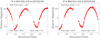 |
Fig. 5 Example synthetic light curves generated with two shape models of asteroid (85990) 1999 JV6 (blue lines) plotted over observational data (red dots) presented as a function of rotational phase. Light-curve details can be found in Table 1. The light curve has a peak-to-peak amplitude of 1.25 mag and displays two sharp minima characteristic of an elongated object. Left panel: fit of the convex light-curve inversion model, rightpanel: best-fit radar shape model. The model summary is given in Table 3. |
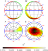 |
Fig. 6 Results of the two-ellipsoid pole search using a combination of radar and light-curve data for asteroid (85990) 1999 JV6 projected on the celestial sphere described in ecliptic coordinates. The best-fit pole is located at ecliptic longitude λ = 144° and latitude λ = −84°. Legend for this figure is the same as for Fig. 2. |
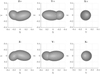 |
Fig. 7 Same as Fig. 3, but for the vertex realisation of the best-fit two-ellipsoid shape model of (85990) 1999 JV6 before the shape details were refined. The X, Y, and Z axes are in kilometres. The model was produced as a result of a pole search using radar data, and has the pole located at λ = 144°, β = − 84°. |
3.3 Refined radar model
The two-ellipsoid shape models give a good approximation of the general shape properties of JV6. However, in order to reproduce the full surface details present in the radar images of JV6 we needed a more complex description. There is an indentation to the larger lobe that can be seen for example in the Goldstone imaging sequence taken on 8 January 2016 (top panel in Fig. 4, and Fig. A.11) with a 1– 2 pixel (18.7–37.4 m) depth. The smaller lobe does not appear perfectly spherical, but rather angular, for example in the images taken at Arecibo on 17 January 2016 (bottom panel in Fig. 4, and Fig. A.21).
The next step in the model optimisation was then the realisation of the shape model with a triangular mesh. The mesh is described in SHAPE as a set of triangular facets with vertices for which positions can be optimised. The vertex adjustments lead to deformations of the triangular facets, modifying both their sizes and orientations, allowing themodel to reproduce smaller surface features. The vertices were initially located across both the ellipsoid components and on the “neck” region connecting them. The vertex positions could be modified by SHAPE by moving them along pre-determined directions (here selected to be normal to the surface of the original two-ellipsoid model).
For further refinement we selected only a subset of our two-ellipsoid models. We picked 15 shape models with χ2 values less than 1% above the minimum value, as well as the model with the spin axis located exactly at the south pole of the celestial sphere. Each of the models was realised as a triangular mesh with a different number of vertices, between 489 and 495, arranged into 974 to 986 triangular facets for each model, with an average length of a facet edge being ~ 20 m. All of the models were optimised by allowing the position of each vertex to vary along with the sidereal rotation period. An extended radar data set was used during the optimisation in order to maximize the yield of information on shape details. Full details of the radar imaging frames used at this stage are listed in Table A.1.
After performing the full fit using the vertex realisation of selected models, we reassessed the pole solution. The best-fit model corresponds to a slightly shifted pole compared to the outcome of the two-ellipsoid pole search. The final shape model, that gives the best fit to the data, has the rotation pole located at λ = 132° and β = −86°, and sidereal period P = 6.536787 h as described in Table 3. The model projections are shown in Fig. 8. The fully realized shape model demonstrates some interesting additional features. There is a prominent indentation in the larger lobe towards the positive end of X-axis and negative end of Y -axis, and the smaller lobe seems flattened at the negative end of the X-axis.
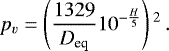
The radar-determined diameter of equivalent-volume sphere is Deq = 442 m, and lies within the uncertainty of the earlier Spitzer and WISE infrared measurement (Mueller et al. 2011; Mainzer et al. 2011), although the object is very elongated. The optical albedo, pv, can be determined knowing the diameter and absolute magnitude, H, using the following relation by Fowler & Chillemi (1992):
 (1)
(1)
Using H = 20.2 from the Minor Planer Center1, we estimate pv = 0.075, which is in agreement with the Spitzer and WISE measurements. Details of the geometric properties of the shape are collected in Table 4.
Some examples of the quality of the fit of the radar-derived model to the data can be seen in Fig. 4. We present all of the radar cw spectra compared to the model-generated spectra in Figs. A.3–A.6 and the radar images used in shape modelling compared to synthetic echoes from this model in Figs. A.7–A.24. Full details of the radar spectra and of the imaging frames are listed in Table A.1.
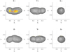 |
Fig. 8 Sameas Fig. 3, but for the best-fit final radar shape model of (85990) 1999 JV6. The X, Y, and Z axes are in kilometres. This model best reproduces the combined light curve and radar data set, with the rotation pole located at λ = 132°, β = −86 °, corresponding to a solution with a χ2 within 1% of the best solution from the search depicted in Fig. 6. Combining radar with optical light-curve data provides excellent viewing geometry coverage, meaning more than 99% of the asteroid surface was observed. The red areas represent the surface elements that were not observed by either radar imaging or light curves. The yellow colour marks regions that were not observed by radar but were observed using light curves. The ‘Y-’ view shows an indentation in the largerlobe. |
Summary of shape parameters for asteroid (85990) 1999 JV6.
3.4 Radar properties of JV6
The radar data can also be a valuable tool for surface characterisation. The radar echo is received in two channels: one records in the same circular (SC) polarisation sense as the transmitted signal, the other in the opposite circular (OC) polarisation sense. Generally the SC-to-OC ratio (SC/OC) is considered a measure of the surface roughness, as strong echo power in the SC polarization can only arise from the transmitted radar signal being scattered by wavelength-scale surface features such as grooves or craters or wavelength-scale particles in the near-surface of the asteroid.
The SC/OC ratio for JV6 from the Arecibo cw observation varies between 0.307 and 0.442 which would suggest varying surface roughness at the scale of the radar wavelength (13 cm), but without clear rotation phase dependency (see Fig. 9 and Table 5). The SC/OC on 16 January 2015, 0.208, at rotation phase 165°, appears anomalous. The SC/OC at the rotation phases 139° and 175° are 0.332 and 0.409, respectively. Because there are no apparent anomalies in the variation of the OC radar cross section as a function of the rotation phase, the anomaly points to a false SC radar cross section on that day. This is likely due to noise, which is greater in the SC than the OC polarization.
There is only a limited sample of Xk-class asteroids for which the SC/OC ratio is published, so it is difficult to compare JV6 with its taxonomic class. The mean value of the SC/OC ratio for JV6 is 0.37 ± 0.05. Other known NEAcontact-binaries in this specific two-ellipsoid arrangement have slightly lower mean SC/OC ratios; for Itokawa this is 0.27 ± 0.04 (Ostro et al. 2004) and for 1996HW1 0.29 ± 0.03 (Magri et al. 2011), which would imply slightly higher wavelength-scale roughness for JV6 than for those two objects. However, those asteroids are of a different taxonomic class than JV6. The mean value of the SC/OC ratio for a NEA is 0.34 ± 0.25 with a median 0.26 (Benner et al. 2008). Therefore, JV6 is a typical representative of the NEA population.
Having determined a 3D shape model for the asteroid, we were also able to derive the radar albedos using the Arecibo cw spectra (see Table 5). The radar albedo in the OC polarization has the mean value of 0.14 ± 0.02. Its variation, between 0.117 and 0.171, is directly proportional to the projected area, which strongly suggests localised variations in the surface structure: either the near-surface bulk density or rubble size distribution. Radar albedo measurements – available for only a few Xk asteroids– span a wide range of values, and the albedo of JV6 falls within that range (Shepard et al. 2010). For NEAs the mean is 0.215 ± 0.016 (based on detections for 213 objects observed from 1998 to June 2016), with a median value of 0.153. Therefore, the value for JV6 does not deviate from this distribution.
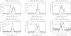 |
Fig. 9 Example cw observations of (85990) 1999 JV6, collected in January 2015 at Arecibo (detailed description of the radar power spectra is in Table A.1). The signal is recorded in two channels, with the same circular (SC) polarisation as the transmitted radiation marked with a dashed line in each panel, and the opposite circular (OC) polarisation, marked with a solid line. The spectra show a SC/OC ratio typical for a NEA, which suggests the presence of some surface features at a scale comparable to the radar wavelength (13 cm for Arecibo). |
4 Searching for the signature of YORP
The spin-state analysis involves investigation of the timing of light-curve observations. The light curves can be represented in the time domain or in rotation phase, φ, when the sidereal rotation period, P, and thus rotation rate, ω, is known. Accounting for the linear change of rotation rate with time, ν, the rotation phase of an asteroid can be expressed for any given time as
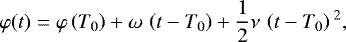 (2)
(2)
where:
t the time of observation (JD),
φ(t) rotation phase in radians,
T0 the epoch from which the model is propagated, also the time (JD) at which the X-axis of the body crosses the plane-of-sky if φ(T0) = 0,
φ(T0) initial rotation phase in radians (rotational offset between the position of X-axis and the plane-of-sky at T0),
ω rotation rate in rad day−1; ω ≡ 2π P, P is rotation period in days,
ν the change of rotation rate in rad day−2; ν ≡  (i.e. the YORP strength).
The linear change of rotation rate can be attributed to the spin component of the YORP torque (Rubincam 2000), referred to herein as the YORP factor. In the presence of non-zero ν the rotational sidereal period value, P, would be interpreted as the initial period valid at T0 which then gradually changes with time.
Radar-derived disc-integrated properties for the cw spectra of (85990) 1999 JV6.
4.1 Convex inversion search
We took two approaches to determining whether the characteristic signature of YORP could be detected in the data available for JV6. First, we used a light-curve-only approach based on the convex inversion methods described in Sect. 3.1. The light-curve-only pole search was repeated for a range of possible YORP factors between − 4 × 10⁻⁷ and 4.5 × 10⁻⁷ rad day−2. For each value of ν we tested a 5° × 5° grid of pole positions, keeping the pole position fixed but optimising the shape and sidereal rotation period at T0. In other words, we performed multiple pole searches assuming different strengths of YORP spin-up, creating multiple χ2 -surfaces by projecting χ2-values obtained for each grid point onto the celestial sphere (Fig. 2 illustrates an example χ2 -surface, with ν = 0). We investigated a χ2 -surface for each value of YORP for the possibility of multiple minima, and then extracted the minimum χ2 value from each of the χ2 -surfaces, with the results shown in Fig. 10. The best fit to the light-curve set for JV6 was obtained for a shape model developed assuming a slight spin-up with ν = 2 × 10⁻⁸ rad day−2, and the YORP acceleration could be between ν = −1 × 10⁻⁸ rad day−2 and ν = 8.5 × 10⁻⁸ rad day−2 (which would produce a rotational phase offset relative to a constant-period solution between 3° and 25° over the approximately ten-year period over which JV6 was observed). However, the constant period solution with ν = 0 reproduced the light curves well (example light-curve fits are shown in Fig. 5 and the full set of light curves in Fig. A.1), with the χ2 differing by approximately 1% from the best-fit model allowing a spin-up. Detecting YORP using light-curve data alone would require a much longerobservation span, but we determine the following upper limit for rotational spin-up for JV6: ν < 8.5 × 10⁻⁸ rad day−2.
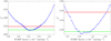 |
Fig. 10 Results of the YORP search for asteroid (85990) 1999 JV6, based on the convex-light-curve-inversion procedures described in Sect. 3.1. For a set of YORP factors a grid of possible pole positions was tested with shape and period optimised at each point. The quality of the fit, χ2, was recorded and the smallest value of χ2 from each search is plotted here against the YORP factor. Left: full range of YORP factors investigated, right: zoomed-in view of the region around the minimum χ2 values. A YORP-induced spin-up of 2 × 10⁻⁸ rad day2 gives the best fit to the light-curve data, but the constant period solution cannot be discarded. The horizontal lines mark the increases above the best-fit χ2 minimum: + 1% (green) and + 10% (red). |
4.2 A radar-shape-model-based approach to searching for YORP
In the second approach to searching for a YORP signature we measured the rotational phase offsets between all of the available light curves (described in Table 1) and the synthetic light curves generated using the best radar-derived shape model. A subset of the light-curve data from 2015 to 2016 was used in the radar shape modelling; the model used was not therefore entirely independent of the light-curve data collected. We reverse-propagated the model from the T0 set in February 2016 and using the model sidereal rotation period to reproduce the light curves at the time of each observation. Individual light-curve fits corresponding to the best radar-derived model for the full data set are shown in Fig. A.2. The fit to the light-curve data is comparable to the light-curve-inversion model, however the minima are sometimes better reproduced, as is the case for the light curve obtained with INT on 4 February 2016, as shown in Fig. 5.
We then measured any additional shift in the rotation phase required to align the model with observations. A deviation of the measured offsets from 0° can be a result of inaccuracy in sidereal period determination or indicate the presence of YORP. A straight line is expected for a constant period solution for all of the measurements. Phase offsets showing a quadratic trend would indicate detection of a YORP acceleration, as seen for example for (25143) Itokawa (Lowry et al. 2014), or (54509) YORP (Taylor et al. 2007; Lowry et al. 2007). The phase offsets for each of the light curves, given in degrees, were plotted as a function of the time at which they were collected as shown in Fig. 11.
The rotational phase offsets, Δφ, the difference between the observed rotational phases and rotational phases calculated using the nominal constant-period solution, can be expressed as
 (3)
(3)
Δφ(t) measured rotation phase offset relative to the nominal spin-state solution in radians,
Δφ(T0) error in the initial rotation phase estimation in radians,
Δω error in the determined rotation rate in rad day−1; corresponding error in period estimate ΔP can be calculated as ΔP ≡ P − 2π(2π P + Δω/24).
The constant period solution reproduces all of the light-curve data very well. A small spread can be observed in the phase offset measurements, which are all below 5° (or ≈1% of rotation), and individual offsets lay within the uncertainty in period determination. A linear trend (assuming ν = 0 in Eq. (3)), corresponding to an error in rotation rate determination, ΔP = 6 × 10⁻⁶ h, can be fitted to the observations with standard deviation of the phase offset measurements σ ≈ 1.4°. The term corresponding to the possible error in initial rotation phase for this fit is very small,  . The points from the 2013 NTT observations (around 1000 days prior to T0) seem not to follow the linear trend, but these are short light-curve segments and the phase offset measurement error might be underestimated. The phase offset measurements can also be fitted with a quadratic curve (following Eq. (3)) with ν = (3.1 ± 2.4) × 10−8 rad day−2 with the standard deviation of individualphase offsets σ ≈ 1.2°. The quadratic trend also contains non-negligible linear terms, corresponding to ΔP ≈ 2.1 × 10⁻⁵ h and Δφ(T0) ≈ 1.2°. While mathematically, the uncertainty on the ν estimated this way would suggest a YORP detection, we note that the standard deviation of the fit of the quadratic trend line to the data is comparable to the standard deviation of the constant-period solution. Moreover the ΔP determined assuming the constant period solution is within the uncertainty of period determination and therefore presents a feasible explanation of the observed phase offsets. Lastly, the data from 2013 present outliers to both trends, and hence can be attributed to neither YORP nor error in period. Therefore, we recommend further photometric observations to evaluate whether theobserved phase offsets will follow the quadratic, and hence lead to a YORP detection, or the linear trend.
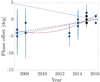 |
Fig. 11 Phase offset measurements for the non-convex radar-derived shape model of asteroid (85990) 1999 JV6, with λ = 132 °, β = −86 °, period P = 6.536787 h, and starting point T0 = 2457425.214 (February 2016). The phase offsets are expressed in degrees with the year of observation on the horizontal axis. The blue squares represent measurements for individual light curves. The phase offsets of the light curves utilised in combination with radar data for shape modelling are marked with black circles. The blue dotted lines indicate the possiblespread in phase offsets due to uncertainty in the measured sidereal period alone, i.e. the uncertainty is 7 × 10⁻⁶ h. The solid red line marks the best-fit YORP solution with ν = (3.1 ± 2.4) × 10−8 rad day−2, (with a standard deviation of the quadratic function fit to the data of σ ≈ 1.2°). The black dashed line marks best fit, assuming a constant-period (zero-YORP) solution (the gradient of the line corresponds to an error in the sidereal period of 6 × 10⁻⁶ h with a standard deviation of the line fit to the data of σ ≈ 1.4°). |
5 Discussion and summary of main conclusions
We have developed a robust shape and spin-state model of JV6 by combining extensive light-curve data and radar measurements. The model features have an effective resolution of about 20 m. The light-curve-only analysis gives an upper limit for YORP detection at 8.5 × 10⁻⁸ rad day−2. Combining the light-curve data with radar observations might suggest a YORP-induced spin-up of ν = (3.1 ± 2.4) × 10−8 rad day−2 when assuming a variable period solution. However, a constant period model could be fit to the combined data set equally well at the 1.5 sigma level. Therefore, more photometric observations are required to confirm or fully reject the possibility of YORP effect acting on this asteroid. The shape model developed with data across a short time span provides an important “anchor” for future measurements. The data collected would not be used to further inform the shape modelling process, but simply to determine any phase offsets from the existing model.
We have shown that JV6 is a bilobed body, a representative of a class of asteroids called contact binaries. The contact binaries are estimated to make up between 15 and 35% of the NEA population (Benner et al. 2006, 2015; Jacobson et al. 2016). The estimated sizes of the NEA contact-binary population are based on reported radar detections of such asteroids, and not on the results of detailed shape modelling. Radar shape models are available for a few asteroids in perceived contact-binary configuration, for example (4769) Castalia (Hudson & Ostro 1994), (2063) Bacchus (Benner et al. 1999), (4179) Toutatis (Hudson et al. 2003), and (4486) Mithra (Brozovic et al. 2010). However, only two of the NEAs modelled so far display distinct ellipsoidal components of different sizes with the smaller near-spherical lobe placed close to the end of the larger, more elongated prolate lobe, similar to what we see for JV6. The first, (8567) 1996 HW1 (Magri et al. 2011), has a clear neck region separating the components. This physical division between two lobes suggests that the asteroid might indeed be made up of two separate bodies that could have slowly collided to form the bilobed shape. The second example is (25143) Itokawa for which an elongated shape was deduced from radar images (Ostro et al. 2004). Later, its contact binary nature was recognised with spacecraft imagery (Demura et al. 2006). The different densities of the two lobes of Itokawa were deduced with the aid of YORP measurements (Lowry et al. 2014). Therefore, JV6 is only the third example where a detailed shape model is available for a body clearly made up of ellipsoidal components in this configuration.
The shape model developed here could be used to study the formation mechanism of a contact binary system. The current spin-state of JV6 with a high obliquity of 173.8°, close to an end state of YORP-induced obliquity shift, suggests a highly evolved system. According to contact-binary formation theory the two components possibly collapsed to form one body due to B-YORP shrinking their mutual orbit (Scheeres 2007; Jacobson & Scheeres 2011). The question is whether the two components were formed through rotational fission from a single parent body, or whether they formed separately. One way to investigate the origin of both components could be through studying the interior structure. This was done for example for asteroid Itokawa (Lowry et al. 2014). In the case of Itokawa, reconciling the theoretical predictions of YORP strength with observations required shifting the centre of mass away from the geometric centre of the figure. The shift was explained with different bulk densities assigned to each lobe. In the case of JV6, the model was developed assuming a principal axis rotation and forcing the centre of mass to be located in the geometric centre of shape. While the model reproduces all of the data very well, a linear offset of the centre of mass might be studied in the future to check whether there is scope for investigation of density inhomogeneity. Further evidence for separate origins for the two apparent components would be in detecting colour or spectral variation between the two lobes.
Recently a different formation scenario was proposed to explain the characteristic morphology demonstrated by Itokawa (Sánchez & Scheeres 2018) that could also be applicable to JV6. The authors investigated the physical evolution of spun-up rubble-pile asteroids with a weak core. In the simulations the asteroids were represented as self-gravitating conglomerates of variable-sizespheres arranged in two concentric layers. The inner layer, the core, was given a weaker tensile strength than the outer layer with other properties like porosity or density remaining constant. A series of spherical aggregates were formed with differently sized cores, with core-to-body radius ratio between 0.5 and 0.9. The synthetic asteroids were then spun up by a series of small increments of the spin rate. It was shown how a rubble-pile body undergoes deformation as the rotation rate increases. The final shapes were dependent on the cohesive strengths of the layers and sizes of the cores. For a small-enough core relative to the asteroid size, and a weak-enough cohesion in the core layer, the deformation is gradual with a dent in the surface emerging first. As the spun-up body stretches, it transitions to a shape resembling a contact binary with a pronounced neck region before braking up into two differently sized ellipsoidal components. The contact binary configuration is apparently stable. It might be that JV6 is a rotationally deformed body currently undergoing the process of rotational fission, rather than one that has already been broken into two bodies and re-formed. The long sidereal rotation period of JV6, seemingly conflicting with this scenario, can be a combined effect of the spin-rate decrease due to change of the inertia tensor and perhaps a YORP-induced slow-down.
Our conclusions can be summarised as follows:
- 1.
The currently available optical and radar data collected over the 11-yr campaign can be successfully reproduced using a constant period solution. However, we estimated an upper limit for YORP detection on JV6 using light-curve data alone. A positive detection of YORP on JV6 would require a much larger data set, so continued photometric monitoring is recommended.
- 2.
The characteristic bilobed shape of JV6 can be a product of either a slow collision of two separately formed components, or a result of an on-going fission process slowed down due to the asteroids deformation. The physical characterisation presented here will enable future studies of the contact-binary NEA population.
Acknowledgements
We thank the referee, Chris Magri, for his comments which helped to improve the manuscript. A.R., S.C.L., S.F.G., C.S., and A.F. acknowledge support from the UK Science and Technology Facilities Council. A.R. and S.C.L. acknowledge support from the South East Physics Network (SEPnet). A.R. acknowledges support from the Royal Astronomical Society (RAS) in the form of a travel grant. B.R. acknowledges support from the RAS in the form of a research fellowship. P.W. acknowledges the U.S. Social Security Administration for financial support. We thank all the staff at the observatories involved in this study for their support, especially James Frederick (Pasadena City College) and Mark Shiffer (Los Angeles Valley College) at the TMO. The Arecibo Observatory is a facility of the National Science Foundation that has been operated under a cooperative agreement by University of Central Florida, Yang Enterprises, Inc., and Universidad Ana G. Méndez since April 2018. During the observations in 2015, 2016 and 2017, Arecibo Observatory was operated by SRI International under a cooperative agreement with Universidad Metropolitana, and the Universities Space Research Association (USRA). The radar observations were fully funded by the National Aeronautics and Space Administration through the Near-Earth Object Observations program through grants No. NNX12AF24G and NNX13AQ46G awarded to USRA. The Arecibo Planetary Radar observations were collected under programmes R2959, R3035, and R3036. The work at the Jet Propulsion Laboratory, California Institute of Technology was performed under contract with the National Aeronautics and Space Administration (NASA). This material is based in part on work supported by NASA under the Science Mission Directorate Research and Analysis Programs. Based in part on observations collected at the European Organisation for Astronomical Research in the Southern Hemisphere under ESO programme 185.C-1033(R). Based in part on observations collected at the Isaac Newton Telescope in Spain (under programmes I/2007A/4 and I/2016A/10) and at the Table Mountain Observatory in USA. The Image Reduction and Analysis Facility software was used for data reduction. The asteroid ephemerides were generated using JPL’s Horizons service. This research has made use of data and services provided by the International Astronomical Union’s Minor Planet Center. This work uses data obtained from the ALCDEF database, which is supported by funding from NASA grant 80NSSC18K0851. We thank Chris Magri for providing the SHAPE software package.
Appendix A Additional figures and table
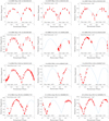 |
Fig. A.1 Same as Fig. 5, but for all available data plotted over synthetic light curves generated with the convex-inversion shape model of asteroid (85990) 1999 JV6. |
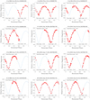 |
Fig. A.1 continued. |
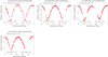 |
Fig. A.1 continued. |
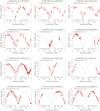 |
Fig. A.2 Same as Fig. 5, but for all available data plotted over synthetic light curves generated with the radar-derived shape model of asteroid (85990) 1999 JV6. |
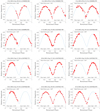 |
Fig. A.2 continued. |
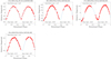 |
Fig. A.2 continued. |
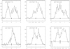 |
Fig. A.3 The cw radar power spectra of asteroid (85990) 1999 JV6 collected at Arecibo in January 2015. Each panel is a graph of echo power in units of standard deviation of the noise against Doppler frequency offset in Hz (relative to centre of mass). The black bar at the 0 Hz frequency has unit length. Each panel is labelled with the date of observations in [yyyymmdd] format. Solid lines represent observations (received OC spectra), and the dashed line is a simulated echo based on the best-fit radar model (see model summary in Table 3). The details of each spectrum are given in Table A.1. |
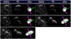 |
Fig. A.7 Similar to Fig. 4, but demonstrating only the fit of the final radar-derived shape model of asteroid (85990) 1999 JV6 to the radar data with detailed image parameters in Table A.1. Each three-image sub-panel ismade of: the observational data (left panel), echo simulated from the best-fit model (middle panel), and plane-of-skyprojection of the best-fit model (right panel). This sequence of images corresponds to the Arecibo data collected on 15 January 2015. |
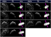 |
Fig. A.8 Same as Fig. A.7, but this sequence of images corresponds to the Arecibo data collected on 16 January 2015. |
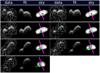 |
Fig. A.9 Same as Fig. A.7, but this sequence of images corresponds to the Arecibo data collected on 17 January 2015. |
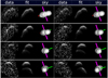 |
Fig. A.10 Same as Fig. A.7, but this sequence of images corresponds to the Arecibo data collected on 18 January 2015. |
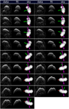 |
Fig. A.11 Same as Fig. A.7, but this sequence of images corresponds to the Goldstone Solar System Radar data collected on 8 January 2016. |
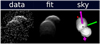 |
Fig. A.12 Same as Fig. A.7, but this image corresponds to the Goldstone Solar System Radar data collected on 9 January 2016. |
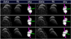 |
Fig. A.13 Same as Fig. A.7, but this sequence of images corresponds to the Goldstone Solar System Radar used for bistatic observations with Green Bank, data collected on 9 January 2016. |
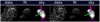 |
Fig. A.14 Same as Fig. A.7, but this sequence of images corresponds to the Goldstone Solar System Radar used for bistatic observations with Green Bank, data collected on 10 January 2016. |
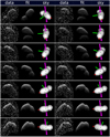 |
Fig. A.15 Same as Fig. A.7, but this sequence of images corresponds to the Goldstone Solar System Radar data collected on 10 January 2016. |
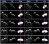 |
Fig. A.16 Same as Fig. A.7, but this sequence of images corresponds to the Goldstone Solar System Radar used for bistatic observations with Green Bank, data collected on 12 January 2016. |
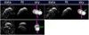 |
Fig. A.17 Same as Fig. A.7, but this sequence of images corresponds to the Goldstone Solar System Radar data collected on 13 January 2016. |
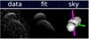 |
Fig. A.18 Same as Fig. A.7, but this image corresponds to the Goldstone Solar System Radar used for bistatic observations with Green Bank, data collected on 13 January 2016. |
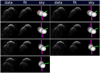 |
Fig. A.19 Same as Fig. A.7, but this sequence of images corresponds to the Arecibo data collected on 14 January 2016. |
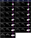 |
Fig. A.20 Same as Fig. A.7, but this sequence of images corresponds to the Arecibo data collected on 15 January 2016. |
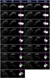 |
Fig. A.21 Same as Fig. A.7, but this sequence of images corresponds to the Arecibo data collected on 17 January 2016. |
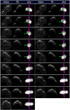 |
Fig. A.22 Same as Fig. A.7, but this sequence of images corresponds to the Arecibo data collected on 18 January 2016. |
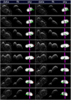 |
Fig. A.23 Same as Fig. A.7, but this sequence of images corresponds to the Arecibo data collected on 19 January 2016. |
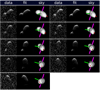 |
Fig. A.24 Same as Fig. A.7, but this sequence of images corresponds to the Arecibo data collected on 15 January 2017. |
Details of radar power spectra and imaging frames used for shape modelling of (85990) 1999 JV6.
References
- Benner, L. A., Hudson, R., Ostro, S. J., et al. 1999, Icarus, 139, 309 [NASA ADS] [CrossRef] [Google Scholar]
- Benner, L. A. M., Nolan, M. C., Ostro, S. J., et al. 2006, Icarus, 182, 474 [NASA ADS] [CrossRef] [Google Scholar]
- Benner, L. A. M., Ostro, S. J., Magri, C., et al. 2008, Icarus, 198, 294 [NASA ADS] [CrossRef] [Google Scholar]
- Benner, L. A. M., Busch, M. W., Giorgini, J. D., Taylor, P. A., & Margot, J.-L. 2015, in Asteroids IV, eds. P. Michel, F. E. DeMeo, & W. F. Bottke (Tucson, AZ: University of Arizona Press), 165 [Google Scholar]
- Binzel, R. P., Harris, A. W., Bus, S. J., & Burbine, T. H. 2001, Icarus, 151, 139 [NASA ADS] [CrossRef] [Google Scholar]
- Bottke, Jr., W. F., Vokrouhlický, D., Rubincam, D. P., & Broz, M. 2002, in Asteroids III, eds. W. F. Bottke, A. Cellino, P. Paolicchi, & R. P. Binzel (Tucson, AZ: University of Arizona Press), 395 [Google Scholar]
- Brozovic, M., Benner, L. A. M., Magri, C., et al. 2010, Icarus, 208, 207 [NASA ADS] [CrossRef] [Google Scholar]
- Bus, S. 1999, PhD Thesis, Massachusetts Institute of Technology [Google Scholar]
- Bus, S. J., & Binzel, R. P. 2002, Icarus, 158, 146 [NASA ADS] [CrossRef] [Google Scholar]
- Buzzoni, B., Delabre, B., Dekker, H., et al. 1984, The Messenger, 38, 9 [NASA ADS] [Google Scholar]
- Chesley, S. R., Ostro, S. J., Vokrouhlický, D., et al. 2003, Science, 302, 1739 [NASA ADS] [CrossRef] [Google Scholar]
- Ćuk, M., & Burns, J. A. 2005, Icarus, 176, 418 [NASA ADS] [CrossRef] [Google Scholar]
- Demura, H., Kobayashi, S., Nemoto, E., et al. 2006, Science, 312, 1347 [NASA ADS] [CrossRef] [Google Scholar]
- Ďurech, J., Vokrouhlický, D., Kaasalainen, M., et al. 2008, A&A, 489, L25 [NASA ADS] [CrossRef] [EDP Sciences] [Google Scholar]
- Ďurech, J., Sidorin, V., & Kaasalainen, M. 2010, A&A, 513, A46 [NASA ADS] [CrossRef] [EDP Sciences] [Google Scholar]
- Ďurech, J., Vokrouhlický, D., Baransky, A. R., et al. 2012, A&A, 547, A10 [NASA ADS] [CrossRef] [EDP Sciences] [Google Scholar]
- Ďurech, J., Vokrouhlický, D., Pravec, P., et al. 2018, A&A, 609, A86 [NASA ADS] [CrossRef] [EDP Sciences] [Google Scholar]
- Fowler, J. W., & Chillemi, J. R. 1992, IRAS asteroid data processing, Phillips Laboratory, Hanscom AF Base, MA), 17 [Google Scholar]
- Golubov, O., Scheeres, D. J., & Krugly, Y. N. 2014, ApJ, 794, 22 [NASA ADS] [CrossRef] [Google Scholar]
- Hudson, S. 1994, Remote Sens. Rev., 8, 195 [CrossRef] [Google Scholar]
- Hudson, R. S., & Ostro, S. J. 1994, Science, 263, 940 [NASA ADS] [CrossRef] [Google Scholar]
- Hudson, R. S., Ostro, S. J., & Scheeres, D. J. 2003, Icarus, 161, 346 [NASA ADS] [CrossRef] [Google Scholar]
- Jacobson, S. A., & Scheeres, D. J. 2011, Icarus, 214, 161 [NASA ADS] [CrossRef] [Google Scholar]
- Jacobson, S. A., Marzari, F., Rossi, A., & Scheeres, D. J. 2016, Icarus, 277, 381 [NASA ADS] [CrossRef] [Google Scholar]
- Kaasalainen, M., & Torppa, J. 2001, Icarus, 153, 24 [NASA ADS] [CrossRef] [Google Scholar]
- Kaasalainen, M., Torppa, J., & Muinonen, K. 2001, Icarus, 153, 37 [NASA ADS] [CrossRef] [Google Scholar]
- Kaasalainen, M., Ďurech, J., Warner, B. D., Krugly, Y. N., & Gaftonyuk, N. M. 2007, Nature, 446, 420 [NASA ADS] [CrossRef] [PubMed] [Google Scholar]
- Lagage, P. O., Pel, J. W., Authier, M., et al. 2004, The Messenger, 117, 12 [NASA ADS] [Google Scholar]
- Lowry, S. C., Fitzsimmons, A., Pravec, P., et al. 2007, Science, 316, 272 [NASA ADS] [CrossRef] [PubMed] [Google Scholar]
- Lowry, S. C., Weissman, P. R., Duddy, S. R., et al. 2014, A&A, 562, A48 [NASA ADS] [CrossRef] [EDP Sciences] [Google Scholar]
- Magri, C., Ostro, S. J., Scheeres, D. J., et al. 2007, Icarus, 186, 152 [NASA ADS] [CrossRef] [Google Scholar]
- Magri, C., Howell, E. S., Nolan, M. C., et al. 2011, Icarus, 214, 210 [NASA ADS] [CrossRef] [Google Scholar]
- Mainzer, A., Grav, T., Bauer, J., et al. 2011, ApJ, 743, 156 [NASA ADS] [CrossRef] [Google Scholar]
- Mueller, M., Delbo’, M., Hora, J. L., et al. 2011, AJ, 141, 109 [NASA ADS] [CrossRef] [Google Scholar]
- Nolan, M. C., Howell, E. S., Scheeres, D. J., et al. 2019, Geophys. Res. Lett., 46, 1956 [NASA ADS] [CrossRef] [Google Scholar]
- Ostro, S. J., Hudson, R. S., Benner, L. A. M., et al. 2002, in Asteroids III, eds. W. F. Bottke, A. Cellino, P. Paolicchi, & R. P. Binzel (Tucson, AZ: University of Arizona Press), 151 [Google Scholar]
- Ostro, S. J., Benner, L. A. M., Nolan, M. C., et al. 2004, Meteorit. Planet. Sci., 39, 407 [NASA ADS] [CrossRef] [Google Scholar]
- Ostro, S. J., Margot, J.-L., Benner, L. A. M., et al. 2006, Science, 314, 1276 [NASA ADS] [CrossRef] [Google Scholar]
- Rozitis, B., & Green, S. F. 2011, MNRAS, 415, 2042 [NASA ADS] [CrossRef] [Google Scholar]
- Rozitis, B., & Green, S. F. 2012, MNRAS, 423, 367 [NASA ADS] [CrossRef] [Google Scholar]
- Rozitis, B., & Green, S. F. 2013, MNRAS, 433, 603 [NASA ADS] [CrossRef] [Google Scholar]
- Rubincam, D. P. 2000, Icarus, 148, 2 [NASA ADS] [CrossRef] [Google Scholar]
- Sánchez, P., & Scheeres, D. J. 2018, Planet. Space Sci., 157, 39 [NASA ADS] [CrossRef] [Google Scholar]
- Scheeres, D. 2007, Icarus, 189, 370 [NASA ADS] [CrossRef] [Google Scholar]
- Scheeres, D. J., Fahnestock, E. G., Ostro, S. J., et al. 2006, Science, 314, 1280 [NASA ADS] [CrossRef] [Google Scholar]
- Shepard, M. K., Clark, B. E., Ockert-Bell, M., et al. 2010, Icarus, 208, 221 [NASA ADS] [CrossRef] [Google Scholar]
- Stokes, G. H., Evans, J. B., Viggh, H. E. M., Shelly, F. C., & Pearce, E. C. 2000, Icarus, 148, 21 [NASA ADS] [CrossRef] [Google Scholar]
- Taylor, P. A., Margot, J.-L., Vokrouhlický, D., et al. 2007, Science, 316, 274 [NASA ADS] [CrossRef] [PubMed] [Google Scholar]
- Trilling, D. E., Mueller, M., Hora, J. L., et al. 2010, AJ, 140, 770 [NASA ADS] [CrossRef] [Google Scholar]
- Vokrouhlický, D., Nesvorný, D., & Bottke, W. F. 2003, Nature, 425, 147 [NASA ADS] [CrossRef] [PubMed] [Google Scholar]
- Walsh, K. J., Richardson, D. C., & Michel, P. 2008, Nature, 454, 188 [NASA ADS] [CrossRef] [Google Scholar]
- Walsh, K. J., Richardson, D. C., & Michel, P. 2012, Icarus, 220, 514 [NASA ADS] [CrossRef] [Google Scholar]
- Warner, B. D. 2014, Minor Planet Bull., 41, 157 [NASA ADS] [Google Scholar]
- Warner, B. D. 2015, Minor Planet Bull., 42, 172 [NASA ADS] [Google Scholar]
- Warner, B. D., Stephens, R. D., & Harris, A. W. 2011, Minor Planet Bull., 38, 172 [NASA ADS] [Google Scholar]
All Tables
A chronological list of optical light curves of asteroid (85990) 1999 JV6 used in this study.
Summary of spin-state parameters for (85990) 1999 JV6 from light-curve inversion and radar-based approaches.
Details of radar power spectra and imaging frames used for shape modelling of (85990) 1999 JV6.
All Figures
|
Fig. 1 Asteroid (85990) 1999 JV6 observing geometries during the optical and radar observations. The graphs display different quantities as a function of time. Top two panels: positions of the object in the ecliptic coordinate system, latitude and longitude, as observed from Earth. Bottom two panels: phase angle, the angle between the positions of the Earth and Sun as observed from the target, and geocentric distance to the target. Optical light curve data from the NTT are marked with filled black circles, with light-curve data from supporting campaigns marked with filled green circles. Red squares represent the published light-curve data. The black cross symbols mark when the Arecibo radar data were collected, and the red crosses mark Goldstone observations. The black continuous line represents the ephemeris of the object. The break in the Y -axis in all four graphs indicates the gap between June 2008 and July 2012. |
| In the text | |
|
Fig. 2 Results of the convex light-curve inversion pole search for asteroid (85990) 1999 JV6, projected on the celestial sphere described in ecliptic coordinates. The blue line marks the ecliptic plane with latitude β = 0°, with some additional circles of latitude marked with black lines and labelled with blue numerals. The red line marks longitude λ = 0° and the green line λ = 180°, with selected meridians marked with black lines and labelled with red numerals. From top-left clockwise, the projections show the eastern (E), western (W), southern (S), and northern (N) hemispheres of the sky, with coordinates of the central point in each projection being (λ = 90 °, β = 0°), (λ = 270 °, β = 0°), (β = −90 °), and (β = +90°). The colour changes from black at the minimum χ2 through red to yellow for higher values of χ2, and the white region represents all the solutions with χ2 more than 50% above the minimum χ2. |
| In the text | |
|
Fig. 3 Best-fit convex shape model of (85990) 1999 JV6. The model was produced as a result of a pole search using light-curve data only, assuming a zero-YORP (constant period) solution, and has the pole located at λ = 55°, β = − 75°. Top row (leftto right): views along the Z, Y and X axes of the body-centric coordinate frame from the positive end of the axis. Bottom row (left to right): views along the Z, Y and X axes from their negative ends. For the model to be physically feasible under the assumption of principal-axis rotation, the Z-axis of the body (also the spin axis) should be aligned with the shortest axis of inertia. There is no relation between the longest axis of inertia and the X-axis of the body, instead the X-axis is arbitrarilyselected so that it would be in the plane of the sky at T0. The units onthe X, Y, and Z axes are arbitrary, as the light-curve convex inversion model is not scaled in size. |
| In the text | |
|
Fig. 4 Comparison of fits of the convex-light-curve-inversion and best-fit radar shape models of asteroid (85990) 1999 JV6 to an example subset of the radar imaging data (the model is summarised in Table 3). Each five-image subpanel is made of: plane-of-sky projection of the convex-light-curve-inversion model (sky 1), the synthetic echo generated using the convex model (fit 1), the observational data (data), echo simulated from the radar best-fit model (fit 2), and plane-of-sky projection of the radar best-fit model (sky 2). The convex model was scaled to have approximately the same volume as the radar model. While the convex-light-curve-inversion model reproduces the light-curve data fairly well (which are fully illustrated in Fig. A.1) and even some general shape properties seen in the radar echoes it fails to reproduce the obvious bifurcation of JV6. On the data and synthetic-echo images the delay increases downwards and the frequency (Doppler) to the right. The plane-of-sky images are orientated with celestial north (in equatorial coordinate system) to the top and east to the left. The principal axes of inertia are marked with coloured rods (red for axis of minimum inertia, green for intermediate axis), and the rotation vector (Z-axis of body-fixed coordinate system, roughly aligned with axis of maximum inertia) is marked with a purple arrow. We highlight the fact that the rotation axis and Z-axis of the bodyoverlap with the axis of maximum inertia. The images were taken, from top to bottom, with: Goldstone on 2016-01-08 08:46:38, Goldstone and GBT on 2016-01-09 06:18:39, Goldstone+GBT on 2016-01-12 06:58:17, Goldstone+GBT on 2016-01-12 08:10:03, Arecibo on 2016-01-17 03:52:07. |
| In the text | |
|
Fig. 5 Example synthetic light curves generated with two shape models of asteroid (85990) 1999 JV6 (blue lines) plotted over observational data (red dots) presented as a function of rotational phase. Light-curve details can be found in Table 1. The light curve has a peak-to-peak amplitude of 1.25 mag and displays two sharp minima characteristic of an elongated object. Left panel: fit of the convex light-curve inversion model, rightpanel: best-fit radar shape model. The model summary is given in Table 3. |
| In the text | |
|
Fig. 6 Results of the two-ellipsoid pole search using a combination of radar and light-curve data for asteroid (85990) 1999 JV6 projected on the celestial sphere described in ecliptic coordinates. The best-fit pole is located at ecliptic longitude λ = 144° and latitude λ = −84°. Legend for this figure is the same as for Fig. 2. |
| In the text | |
|
Fig. 7 Same as Fig. 3, but for the vertex realisation of the best-fit two-ellipsoid shape model of (85990) 1999 JV6 before the shape details were refined. The X, Y, and Z axes are in kilometres. The model was produced as a result of a pole search using radar data, and has the pole located at λ = 144°, β = − 84°. |
| In the text | |
|
Fig. 8 Sameas Fig. 3, but for the best-fit final radar shape model of (85990) 1999 JV6. The X, Y, and Z axes are in kilometres. This model best reproduces the combined light curve and radar data set, with the rotation pole located at λ = 132°, β = −86 °, corresponding to a solution with a χ2 within 1% of the best solution from the search depicted in Fig. 6. Combining radar with optical light-curve data provides excellent viewing geometry coverage, meaning more than 99% of the asteroid surface was observed. The red areas represent the surface elements that were not observed by either radar imaging or light curves. The yellow colour marks regions that were not observed by radar but were observed using light curves. The ‘Y-’ view shows an indentation in the largerlobe. |
| In the text | |
|
Fig. 9 Example cw observations of (85990) 1999 JV6, collected in January 2015 at Arecibo (detailed description of the radar power spectra is in Table A.1). The signal is recorded in two channels, with the same circular (SC) polarisation as the transmitted radiation marked with a dashed line in each panel, and the opposite circular (OC) polarisation, marked with a solid line. The spectra show a SC/OC ratio typical for a NEA, which suggests the presence of some surface features at a scale comparable to the radar wavelength (13 cm for Arecibo). |
| In the text | |
|
Fig. 10 Results of the YORP search for asteroid (85990) 1999 JV6, based on the convex-light-curve-inversion procedures described in Sect. 3.1. For a set of YORP factors a grid of possible pole positions was tested with shape and period optimised at each point. The quality of the fit, χ2, was recorded and the smallest value of χ2 from each search is plotted here against the YORP factor. Left: full range of YORP factors investigated, right: zoomed-in view of the region around the minimum χ2 values. A YORP-induced spin-up of 2 × 10⁻⁸ rad day2 gives the best fit to the light-curve data, but the constant period solution cannot be discarded. The horizontal lines mark the increases above the best-fit χ2 minimum: + 1% (green) and + 10% (red). |
| In the text | |
|
Fig. 11 Phase offset measurements for the non-convex radar-derived shape model of asteroid (85990) 1999 JV6, with λ = 132 °, β = −86 °, period P = 6.536787 h, and starting point T0 = 2457425.214 (February 2016). The phase offsets are expressed in degrees with the year of observation on the horizontal axis. The blue squares represent measurements for individual light curves. The phase offsets of the light curves utilised in combination with radar data for shape modelling are marked with black circles. The blue dotted lines indicate the possiblespread in phase offsets due to uncertainty in the measured sidereal period alone, i.e. the uncertainty is 7 × 10⁻⁶ h. The solid red line marks the best-fit YORP solution with ν = (3.1 ± 2.4) × 10−8 rad day−2, (with a standard deviation of the quadratic function fit to the data of σ ≈ 1.2°). The black dashed line marks best fit, assuming a constant-period (zero-YORP) solution (the gradient of the line corresponds to an error in the sidereal period of 6 × 10⁻⁶ h with a standard deviation of the line fit to the data of σ ≈ 1.4°). |
| In the text | |
|
Fig. A.1 Same as Fig. 5, but for all available data plotted over synthetic light curves generated with the convex-inversion shape model of asteroid (85990) 1999 JV6. |
| In the text | |
|
Fig. A.1 continued. |
| In the text | |
|
Fig. A.1 continued. |
| In the text | |
|
Fig. A.2 Same as Fig. 5, but for all available data plotted over synthetic light curves generated with the radar-derived shape model of asteroid (85990) 1999 JV6. |
| In the text | |
|
Fig. A.2 continued. |
| In the text | |
|
Fig. A.2 continued. |
| In the text | |
|
Fig. A.3 The cw radar power spectra of asteroid (85990) 1999 JV6 collected at Arecibo in January 2015. Each panel is a graph of echo power in units of standard deviation of the noise against Doppler frequency offset in Hz (relative to centre of mass). The black bar at the 0 Hz frequency has unit length. Each panel is labelled with the date of observations in [yyyymmdd] format. Solid lines represent observations (received OC spectra), and the dashed line is a simulated echo based on the best-fit radar model (see model summary in Table 3). The details of each spectrum are given in Table A.1. |
| In the text | |
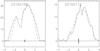 |
Fig. A.4 Same as Fig. A.3, but for the cw spectra collected at Goldstone in January 2016. |
| In the text | |
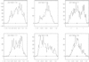 |
Fig. A.5 Same as Fig. A.3, but for the cw spectra collected at Arecibo in January 2016. |
| In the text | |
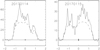 |
Fig. A.6 Same as Fig. A.3, but for the cw spectra collected at Arecibo in January 2017. |
| In the text | |
|
Fig. A.7 Similar to Fig. 4, but demonstrating only the fit of the final radar-derived shape model of asteroid (85990) 1999 JV6 to the radar data with detailed image parameters in Table A.1. Each three-image sub-panel ismade of: the observational data (left panel), echo simulated from the best-fit model (middle panel), and plane-of-skyprojection of the best-fit model (right panel). This sequence of images corresponds to the Arecibo data collected on 15 January 2015. |
| In the text | |
|
Fig. A.8 Same as Fig. A.7, but this sequence of images corresponds to the Arecibo data collected on 16 January 2015. |
| In the text | |
|
Fig. A.9 Same as Fig. A.7, but this sequence of images corresponds to the Arecibo data collected on 17 January 2015. |
| In the text | |
|
Fig. A.10 Same as Fig. A.7, but this sequence of images corresponds to the Arecibo data collected on 18 January 2015. |
| In the text | |
|
Fig. A.11 Same as Fig. A.7, but this sequence of images corresponds to the Goldstone Solar System Radar data collected on 8 January 2016. |
| In the text | |
|
Fig. A.12 Same as Fig. A.7, but this image corresponds to the Goldstone Solar System Radar data collected on 9 January 2016. |
| In the text | |
|
Fig. A.13 Same as Fig. A.7, but this sequence of images corresponds to the Goldstone Solar System Radar used for bistatic observations with Green Bank, data collected on 9 January 2016. |
| In the text | |
|
Fig. A.14 Same as Fig. A.7, but this sequence of images corresponds to the Goldstone Solar System Radar used for bistatic observations with Green Bank, data collected on 10 January 2016. |
| In the text | |
|
Fig. A.15 Same as Fig. A.7, but this sequence of images corresponds to the Goldstone Solar System Radar data collected on 10 January 2016. |
| In the text | |
|
Fig. A.16 Same as Fig. A.7, but this sequence of images corresponds to the Goldstone Solar System Radar used for bistatic observations with Green Bank, data collected on 12 January 2016. |
| In the text | |
|
Fig. A.17 Same as Fig. A.7, but this sequence of images corresponds to the Goldstone Solar System Radar data collected on 13 January 2016. |
| In the text | |
|
Fig. A.18 Same as Fig. A.7, but this image corresponds to the Goldstone Solar System Radar used for bistatic observations with Green Bank, data collected on 13 January 2016. |
| In the text | |
|
Fig. A.19 Same as Fig. A.7, but this sequence of images corresponds to the Arecibo data collected on 14 January 2016. |
| In the text | |
|
Fig. A.20 Same as Fig. A.7, but this sequence of images corresponds to the Arecibo data collected on 15 January 2016. |
| In the text | |
|
Fig. A.21 Same as Fig. A.7, but this sequence of images corresponds to the Arecibo data collected on 17 January 2016. |
| In the text | |
|
Fig. A.22 Same as Fig. A.7, but this sequence of images corresponds to the Arecibo data collected on 18 January 2016. |
| In the text | |
|
Fig. A.23 Same as Fig. A.7, but this sequence of images corresponds to the Arecibo data collected on 19 January 2016. |
| In the text | |
|
Fig. A.24 Same as Fig. A.7, but this sequence of images corresponds to the Arecibo data collected on 15 January 2017. |
| In the text | |
Current usage metrics show cumulative count of Article Views (full-text article views including HTML views, PDF and ePub downloads, according to the available data) and Abstracts Views on Vision4Press platform.
Data correspond to usage on the plateform after 2015. The current usage metrics is available 48-96 hours after online publication and is updated daily on week days.
Initial download of the metrics may take a while.