| Issue |
A&A
Volume 631, November 2019
|
|
|---|---|---|
| Article Number | A108 | |
| Number of page(s) | 34 | |
| Section | Interstellar and circumstellar matter | |
| DOI | https://doi.org/10.1051/0004-6361/201935785 | |
| Published online | 05 November 2019 | |
VLTI/PIONIER survey of disks around post-AGB binaries
Dust sublimation physics rules★,★★
1
Instituut voor Sterrenkunde (IvS), KU Leuven,
Celestijnenlaan 200D, 3001 Leuven, Belgium
e-mail: This email address is being protected from spambots. You need JavaScript enabled to view it.
2
Université Grenoble Alpes, CNRS, IPAG,
38000 Grenoble, France
3
Research School of Astronomy and Astrophysics, Australian National University,
Cotter Road, Weston Creek ACT 2611, Australia
4
Department of Physics and Astronomy, Macquarie University,
Sydney, NSW 2109, Australia
5
Department of Astronomy, University of Michigan,
1085 S. University, Ann Arbor, MI 48109, USA
6
Netherlands Institute for Space Research (SRON),
Sorbonnelaan 2, 3584 CA Utrecht, The Netherlands
Received:
26
April
2019
Accepted:
6
September
2019
Abstract
Context. Post-asymptotic giant branch (AGB) binaries are surrounded by circumbinary disks of gas and dust that are similar to protoplanetary disks found around young stars.
Aims. We aim to understand the structure of these disks and identify the physical phenomena at play in their very inner regions. We want to understand the disk-binary interaction and to further investigate the comparison with protoplanetary disks.
Methods. We conducted an interferometric snapshot survey of 23 post-AGB binaries in the near-infrared (H-band) using VLTI/PIONIER. We fit the multi-wavelength visibilities and closure phases with purely geometrical models with an increasing complexity (including two point-sources, an azimuthally modulated ring, and an over-resolved flux) in order to retrieve the sizes, temperatures, and flux ratios of the different components.
Results. All sources are resolved and the different components contributing to the H-band flux are dissected. The environment of these targets is very complex: 13/23 targets need models with thirteen or more parameters to fit the data. We find that the inner disk rims follow and extend the size-luminosity relation established for disks around young stars with an offset toward larger sizes. The measured temperature of the near-infrared circumstellar emission of post-AGB binaries is lower (Tsub ~ 1200 K) than for young stars, which is probably due to a different dust mineralogy and/or gas density in the dust sublimation region.
Conclusions. The dusty inner rims of the circumbinary disks around post-AGB binaries are ruled by dust sublimation physics. Additionally a significant amount of the circumstellar H-band flux is over-resolved (more than 10% of the non-stellar flux is over-resolved in 14 targets). This hints that a source of unknown origin, either a disk structure or outflow. The amount of over-resolved flux is larger than around young stars. Due to the complexity of these targets, interferometric imaging is a necessary tool to reveal the interacting inner regions in a model-independent way.
Key words: stars: AGB and post-AGB / techniques: high angular resolution / techniques: interferometric / binaries: general / circumstellar matter / protoplanetary disks
Full Table A.1 is available at the CDS via anonymous ftp to cdsarc.u-strasbg.fr (130.79.128.5) or via http://cdsarc.u-strasbg.fr/viz-bin/cat/J/A+A/631/A108
Based on VLTI observations 093.D-0573 and 094.D-0865.
© ESO 2019
1 Introduction
Binarity is widely present in all kinds of stars (25% of low-mass stars and more than 80% of high-mass stars have at least one companion; Duchêne & Kraus 2013) and binary research constitutes a main domain of stellar astrophysics. Binary evolution gives rise to diverse phenomena, such as thermonuclear novae, supernovae type Ia, sub-luminous supernovae, merger events generating detectable gravitational waves, and objects with lower initial mass, such as sub-dwarf B-stars, barium stars, cataclysmic variables, and asymmetric planetary nebulae (PNe). Understanding the diverse impact of binarity in stellar evolution is therefore crucial but is, also, still poorly understood. In this paper we focus on observations of post-asymptotic giant branch (pAGB) binaries that are objects in fast transition (~105 yr) between the AGB and the PNe stages that are surrounded by a circumbinary disk (Van Winckel 2018).
Binarity plays a central role in the formation of the dusty disks, which were first postulated from the infrared (IR) excess in the spectral energy distribution (SED). These excesses cannot be attributed to expanding detached shells (e.g., de Ruyter et al. 2006). Most of the disk sources were then discovered to be binaries through radial velocity measurements (Van Winckel 2003; Van Winckel et al. 2009; Oomen et al. 2018). Those observations lead to the conclusion that pAGB disks originate from the evolved star’s mass loss via a poorly understood binary interaction mechanism that happens at the end of the AGB phase for low- and intermediate-mass stars (0.8–8 M⊙). Millimeter observations of CO lines with the Plateau de Bure interferometer and the Atacama Large Millimeter/submillimeter Array (ALMA) resolve the outer parts of these disks and show them to be in Keplerian rotation, and thus stable (Bujarrabal et al. 2013, 2015, 2016, 2017, 2018). The CO observations also reveal a disk-wind component, suggesting angular momentum transport in the disk. Dust grains are inferred to have large sizes (ranging from a few microns to millimeter sizes) and a high crystallinity fraction, which is based on analyses of the mid-IR spectral features and sub-mm spectral slopes (de Ruyter et al. 2006; Gielen et al. 2008, 2011; Hillen et al. 2015). The dust masses found in these disks are on the order of 10−4 –10−3 M⊙ (Sahai et al. 2011; Hillen et al. 2014), but are highly model dependent.
Despite very different forming processes, pAGB disks are in many ways (IR excess, Keplerian rotation, winds, dust mass, dust mineralogy and grain sizes) similar to protoplanetary disks (PPDs) around young stellar objects (YSOs). Radiative transfer models of PPDs are able to successfully reproduce both the SED and IR interferometric measurements on the few pAGB targets studied so far (Hillen et al. 2014, 2015, 2017; Kluska et al. 2018). As the PPDs are well studied both observationally and theoretically, the very close similarity with the disks around pAGB binaries points toward a potential universality of physical processes in dusty circumstellar disks that occupy a different parameter space (i.e., different formation process, presumably shorter lifetime, high stellar luminosity). Also, such a similarity between those two types of disks raises the question of the planet formation efficiency in pAGB disks (e.g., Schleicher & Dreizler 2014), especially as several planets are candidates for being formed in such second-generation disks (e.g., NN Ser; Völschow et al. 2014; Marsh et al. 2014; Parsons et al. 2014; Hardy et al. 2016).
The interaction between the binary and the disk gives rise to several complex physical processes. Firstly, these systems show indirect signs for re-accretion from the circumbinary disk onto the central system: the primary’s photospheric spectrum shows depletion in elements that have the highest condensation temperature (Maas et al. 2003; Gezer et al. 2015; Oomen et al. 2018; Kamath & Van Winckel 2019). The scenario explaining this depletion is that the condensed elements are subject to radiative pressure and remain in the disk while the gas is re-accreted onto the central star(s) (Waters et al. 1992). However, this scenario needs to be confirmed by direct observations of the re-accretion.
Secondly, spectral time series observations allowed the detection of bipolar jets linked to the secondary star (e.g., Thomas et al. 2013; Gorlova et al. 2015; Bollen et al. 2017). These jets have their origin around the secondaries which should also be surrounded by an accretion disk. Interestingly, the Very Large Telescope Interferometer (VLTI) observations of one of the most studied pAGB-binaries, IRAS 08544-4431, with the Precision Integrated-Optics Near-infrared Imaging ExpeRiment (PIONIER) in the near-IR, detected a point-source emission at the position of the secondary. It should not be detectable if the emission was coming from a photosphere alone and it was tentatively linked with the circum-secondary accretion disk (Hillen et al. 2016; Kluska et al. 2018). The existence of this unexpected continuum emission from the secondary needs to be investigated in other systems as well.
Third, the orbits of the binaries disagree with predictions of theoretical models. At the end of the AGB phase we expect the period distribution of the binaries to be bimodal: the systems that went through common envelope evolution should result in a shrinkage of their orbital period and wider systems should have larger orbits because of the mass loss of the primary (Nie et al. 2012). However, radial velocity monitoring of the binary orbits revealed that the detected orbital distribution falls between these two modes and show periods that are not predicted by population studies. Moreover, tidal circularization of the orbits is expected when the primary evolves on the giant branches, whereas observations show orbits with nonzero eccentricity values (~0.2–0.3) pointing at an eccentricity pumping mechanism (Oomen et al. 2018). Interactions between the circumbinary disk and the binary could explain some of the observed eccentricities (e.g., Dermine et al. 2013; Vos et al. 2015). However, this mechanism is still debated as strong assumptions were made about the disk radial and vertical structure, disk viscosity and lifetime (Rafikov 2016). Spatially resolved observations of the disk inner rim from which we could infer the radius, height, eccentricity, perturbation will therefore help to constrain hydrodynamic models of disk-binary interactions.
The binary eccentricity can also disturb the circumbinary disk (e.g., Thun et al. 2017). Another possibility is that the orbital eccentricity is pumped-up by an increased mass exchange between the two stars at the periastron passage (grazing envelope evolution, e.g., Kashi & Soker 2018). This mechanism could also delay the common envelope phase extending the final orbital period (Shiber et al. 2017).
Our previous high-spectral resolution time series and high-angular resolution interferometric data enabled us to build an archetype of a pAGB binary system. In our current state of knowledge, its building blocks are likely to be a pAGB primary, a main-sequence secondary surrounded by an accretion disk which launches a wide bipolar jet, a binary orbit that is eccentric and not predicted by population synthesis models, a circumbinary disk with a dust inner rim at a radius of several astronomical units, likely ruled by dust sublimation physics and that is azimuthally perturbed (e.g., Kluska et al. 2018), and a near-IR extended flux from a yet unknown origin. Here, we present an interferometric snapshot survey in the near-IR of 23 systems in order to test this archetype. We focus on the general properties of the different components contributing to the H-band flux in those systems. The paper is organized as follows. We describe the photometric and interferometric observations in Sect. 2 and the geometric models in Sect. 3. We show the results in Sect. 4, discuss them in Sect. 5 before concluding in Sect. 6.
2 Observations
2.1 Photometry
The best photosphere fit to the visible part of the photometry of the sources was used to extrapolate the stellar spectrum to the H-band (1.65 μm). We used the targets photometry of Hillen et al. (2017) and Oomen et al. (2018). We have compiled archival photometry on all our targets except V494 Vel (Fig. F.1). The photometric data is coming from Johnson-Cousins bands (Johnson et al. 1966; Johnson & Mitchell 1975; Morel & Magnenat 1978; Mermilliod et al. 1997; Kharchenko 2001; Ducati 2002; Mermilliod 2006; Richmond 2007; Lasker et al. 2008; Ofek 2008; Anderson & Francis 2012; Nascimbeni et al. 2016; Henden et al. 2016), Geneva photometry (Mermilliod et al. 1997) and Strömgren photometry (Hauck & Mermilliod 1998; Paunzen et al. 2001). For some targets, we also used photometry from Tycho (Høg et al. 2000; Hoeg et al. 1997; Urban et al. 1998) and Gaia (Gaia Collaboration 2016). For near-IR photometry we used 2MASS (Cutri et al. 2003) while for mid and far-IR we used AKARI (Murakami et al. 2007; Ishihara et al. 2010), WISE (Cutri et al. 2012), IRAC (Spitzer Science 2009), IRAS (Helou & Walker 1988) and MSX (Egan et al. 2003).
To fit the SED we have first derived stellar parameters (such as effective temperature, Teff, surface gravity, log g; see Table 1) from existing spectra of the stars (Waelkens et al. 1991; Giridhar et al. 1994, 2000; Van Winckel 1997; Van Winckel et al. 1998; Dominik et al. 2003; Maas et al. 2002, 2003, 2005; de Ruyter et al. 2006)using Kurucz models (Kurucz 1993). We then defined allowed ranges around those values that the fitting algorithm can explore (Teff ± 250 K; log g ± 0.3 or between 0 and 2.5 if not constrained by the spectrum). We then minimized the χ2 via a Levenberg-Marquardt algorithm between the photometric data and the reddened model (the results are displayed in Table F.19).
Binary post-AGB stars in our sample.
2.2 Interferometry
The interferometric observations were obtained with PIONIER located at the VLTI at Mount Paranal in Chile. PIONIER recombines light from four telescopes in the near-IR H-band (between 1.5 and 1.85 μm). The interferometric observables are the squared visibility amplitude (V2), that is a measure of the degree of spatial resolution of the source by a given baseline at a given wavelength, and closure phase (CP), that is a measure of the departure from point-symmetry of the target. The target selection (see Table 1) was based on (1) the identification of the object as a post-AGB star, (2) the presence of an H-band excess (de Ruyter et al. 2006; Gezer et al. 2015) and (3) observability with PIONIER on the VLTI.
Most targets were observed as part of a dedicated observing program (European Southern Observatory (ESO) program 093.D-0573, PI: Hillen), but some were also observed as a supplement to the imaging campaign on IRAS 08544-4431 (ESO program 094.D-0865; PI: Hillen). This explains, to some extent, the diversity in uv -coverage among the sample (see Table A.2). The observations of IRAS 08544-4431 are described in Hillen et al. (2016). Each observation of the science star was bracketed with two calibrator stars to well interpolate the transfer function and calibrate the squared visibilities (V2) and closure phases (CP). The observations were taken using the small (A1-B2-C1-D0), the intermediate (D0-G1-H0-I1), and the extended (A1-G1-J3-K0) configurations depending on the expected size and luminosity of the object. Therefore, not all the targets have observations on the three configurations (see Figs. B.2 and B.2) causing an in-homogeneous (u, v)-coverage throughout the whole dataset. All the targets were observed with a grism, leading to spectrally dispersed data with a low resolution (R ~ 30). We are therefore sensitive to the continuum only. The data was reduced using the pndrs software (Le Bouquin et al. 2011). The entire dataset is available on the Optical interferometry DataBase (OiDB)1.
All the targets have squared visibilities significantly below unity (see Fig. B.1) meaning that at least a fraction of the near-IR emission is spatially resolved in all of them. For several targets the closure phases are showing a nonzero signal indicating departure from point symmetry.
3 Model fitting
In order to analyze the dataset we performed a fitting with geometrical models with increasing complexity. We stress that the dataset is diverse in both the sizes of our targets and the obtained (u, v)-coverage. The challenge is that the observational constraints differ from object to object. Because of the sparsity of the (u, v)-coverages, our models do not take into account any intrinsic variability of the inner source as there is orbital motion and/or large amplitude pulsations. We define several classes of models in Sects. 3.2–3.5. We also describe our fitting strategy in Sect. 3.6. We start by describing in Sect. 3.1 the way these models attribute spectral dependence between the different components.
3.1 Model definition and spectral dependence
Thanks to the linearity property of the Fourier transform, the analytic models are defined in the Fourier plane as a linear combination of different geometrical components. The weights of this combination are the relative fluxes of the components. Those flux contributions are defined as:

where  is the flux ratio of the ith component at 1.65 μm.
In the models there are four possible components: the primary star, the secondary star, the circumbinary ring, and the background. Not all components are present in all the models. To extrapolate the flux ratios over the observed wavelength range the components are assigned with a spectral dependence law (fi).
The spectral dependence of the primary star is taken from the photospheric flux in the H-band from the best-fit from the SED2 and is normalized to unity at 1.65 μm. This is possible as the contribution from the secondary and the ring are negligible in the visible because of their lower temperature and high contrast with the primary. The fluxes of the secondary star and the background are defined as a power-law with wavelength and a spectral index ( ) such that:
 (4)
(4)
where λ is the wavelength of an observation and i is either sec or bg if it is the secondary star or the background, respectively. Finally, the ring spectral dependence is defined as a black body function at a given temperature Tring that is normalized to unity at 1.65 μm:
 (5)
(5)
where BB isthe black body function.
In the following sections the model geometrical descriptions are presented as well as the full model equations.
3.2 Single star and background flux: s0-1
This first set of models includes two components: the star and the background flux.
The star
The star is geometrically defined by the diameter of its uniform disk (UDprim). The stellar visibility Vprim(u, v) is therefore:
 (6)
(6)
where u and v are the coordinates in the Fourier domain and J1 is the first order Bessel function.
The background
The background is the over-resolved flux which means that this component is fully resolved even for the smallest baseline. Its visibility (Vbg) equals 0 for all baselines.
The final model
This is a linear combination of the visibilities of the star and the background with as factors their flux contribution that depend on the observed wavelength (see Sect. 3.1). The spectral dependence of the background is either assumed to be a black-body (model s0) or a power-law (model s1). We made this choice as the s0 model is the starting point to all the models and, in the absence of the ring component, it is already giving a good indication for the temperature of the environment whereas in all the other models the background is modeled as a power-law. The final visibility is expressed as:
 (7)
(7)
Thanks to Eq. (1) we have:
 (8)
(8)
3.3 Single star and a ring: sr0-6
In this set of models there are three components: the primary star, the ring, and the background. The star is modeled as a point source and the circumstellar matter is modeled by a Gaussian ring that can be inclined and modulated, depending on the complexity of the model.
The star
The visibility of a point source is Vprim = 1. The position of the star with respect to the center of the ring is defined by x0 and y0. Because of this shift, the complex visibility of the star is:
 (9)
(9)
where u and v are the spatial frequencies in the west-east and south-north directions.
The ring
The ring is first defined as an infinitesimal ring distribution. Its visibility (Vring0(u, v)) equals to:
 (10)
(10)
where J0 is the Bessel function of the 0th order, θ the diameter of the ring and ρ′ is the spatial frequency of a data point corrected for inclination (inc) and position angle (PA) of the ring such as:
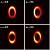 |
Fig. 1 Illustration of four azimuthal modulation coefficients on ring geometry. For each quadrant all modulation parameters are kept to zero apart from the one displayed. The red star shows the center of the ring. |

This ring is then azimuthally modulated using a set of sinusoidal functions having a period 2π and π called first order and second order modulations respectively. The ring visibility with first order modulation (Vring1(u, v)) and with first and second order modulations (Vring2(u, v)) can be written as:
![Mathematical equation: \begin{eqnarray*} V^{\mathrm{ring1}}(u,v) &=& V^{\mathrm{ring0}} -i (c_{\mathrm{1}} \cos\alpha + s_{\mathrm{1}} \sin\alpha) J_{\mathrm{1}}(\pi\rho'\theta), \\[5pt] V^{\mathrm{ring2}}(u,v) &=& V^{\mathrm{ring1}} - (c_{\mathrm{2}} \cos2\alpha + s_{\mathrm{2}} \sin2\alpha) J_{\mathrm{2}}(\pi\rho'\theta), \end{eqnarray*}](/articles/aa/full_html/2019/11/aa35785-19/aa35785-19-eq12.png)
where c1 and s1 are the first order modulation coefficients, c2 and s2 are the second order modulation coefficients, J1 and J2 are the first and second order Bessel functions and α is the azimuthal angle of the ring, starting at the major-axis (see Fig. 1).
Finally, to have a Gaussian ring, one needs to convolve the infinitesimal ring in the image space by a Gaussian, which is equivalent to a multiplication in the Fourier domain:
 (16)
(16)
where δθ is the ratio of the ring full width at half maximum to its radius.
The background
The extended flux is modeled by an over-resolved emission that has a null visibility.
The final model
As the flux ratios of the three components are normalized to 1 at 1.65 μm (Eq. (1)),  is defined as:
 (17)
(17)
The final visibility can therefore be written as a linear combination of the three components of the model such as:
 (18)
(18)
3.4 Binary: b1-2
This set of models is made of two stars and a background flux.
The binary
The two stars are defined as uniform disks (see Eq. (6)). The position of the primary star is defined by the two position parameters (x0, y0) as in Eq. (9). The visibility of the primary star is therefore defined as:
 (19)
(19)
The secondary star is centered at position (0,0) and its visibility equation is identical to Eq. (6):
 (20)
(20)
The final model
The normalization of the fluxes (Eq. (1)) gives:
 (21)
(21)
In this set of models  is therefore not fitted and is computed from the two other flux ratios. The final visibility is therefore:
 (22)
(22)
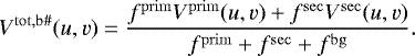
3.5 Binary and a ring: br1-5
The last set of models have four components: the primary, the secondary, a ring, and a background.
The binary
The primary star is defined as a uniform disk which is shifted w.r.t. to the center of the disk by (x0, y0) such as:
 (23)
(23)
The coordinates of the secondary (xsec, ysec) is defined in reference to the coordinates of the primary such as the coordinates of the secondary are:
![Mathematical equation: \begin{eqnarray*} x_{\mathrm{sec}} &=& -rM x_0, \\[5pt] y_{\mathrm{sec}} &=& -rM y_0, \end{eqnarray*}](/articles/aa/full_html/2019/11/aa35785-19/aa35785-19-eq23.png)
where rM is the mass ratio between the primary and the secondary. The visibility of the secondary is:
 (26)
(26)
The binary separation is limited to be lower or equal to one third of the ring diameter projected along the binary separation.
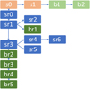 |
Fig. 2 Tree of models. The single star and background models are in orange, the single star and a ring models are in blue, the binary models are in light green and the binary and ring models are in dark green. |
The full model
The flux ratio normalization (Eq. (1)) is as follows:
 (27)
(27)
The ring-to-total flux ratio is therefore not fitted and is recovered from this equation.
The total visibility is therefore:
![Mathematical equation: \begin{align*} V^{\mathrm{tot,br\#}}(u,v,\lambda) = &\,\frac{ f^{\mathrm{prim}}V^{\mathrm{prim}}(u,v) } { f^{\mathrm{prim}} + f^{\mathrm{sec}} + f^{\mathrm{ring}} + f^{\mathrm{bg}} }\\[8pt] &+\,\frac{ f^{\mathrm{sec}} V^{\mathrm{sec}}(u,v) + f^{\mathrm{ring}} V^{\mathrm{ring}}(u,v) } { f^{\mathrm{prim}} + f^{\mathrm{sec}}+ f^{\mathrm{ring}} + f^{\mathrm{bg}} }\nonumber, \end{align*}](/articles/aa/full_html/2019/11/aa35785-19/aa35785-19-eq26.png) (28)
(28)
where Vring(u, v), Vprim(u, v) and Vsec (u, v) are defined from Eqs. (16), (23) and (26) respectively.
3.6 Strategy
Our models are fitted to both V2 and CP. However, there is a large variety of data in our sample as some targets have a signal with low complexity, such as AC Her (#1), but others have a high complexity, such as U Mon (#22). Recent studies of IRAS 08544-4431 (#10) showed that model br5 with 17 parameters is needed to reproduce the interferometric dataset (Hillen et al. 2016). We therefore fit a tree of models, starting with our simplest model (s0, see Sect. 3.2), up to the most complex model (br5, see Sect. 3.5), inspired by Hillen et al. (2016) with 17 parameters. We start by fitting the simplest model to all the targets. We then fit models with increasing complexity using the best parameters from the previous model as the starting point for the next model (adding the new parameters). Some targets are best fitted by models that do not include a ring but just a binary. We therefore included several forks in the model tree (see Fig. 2).
For each model a first fit is performed using a genetic algorithm implemented with DEAP (Fortin et al. 2012). The initial population is defined with a random flat distribution over the initial parameters. For the parameters that are not used in the previous model the distribution spans over all the allowed values of a parameter that we defined in Table 2. For the parameters already used in the previous model in the tree, we span over 30% of its best-fit value for the previous model. The mutation is Gaussian over the parameter allowed distribution and has a probability of 5%. The individual selection is made through a three-rounds tournament. Then, using the best fit from the genetic algorithm as a starting point, a MCMC minimization is performed with the emcee package (Foreman-Mackey et al. 2013) to determine the error bars on the parameters. When a model has a larger χ2 than the previous model in the model tree we redo the minimization as this indicates that a local minimum was reached.
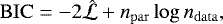
As it is not possible to directly compare two models with a different number of parameters, we wanted to use a criterion that is applicableto all our sample. Such criteria exists from information theory and we used the Bayesian information criterion (BIC; Schwarz 1978) to select the best model for each target. This criteria aims to infer the model that fits the data the best without over fitting and is used in several studies of stellar physics to infer the most likely model that reproduce the data from a set of different models (e.g., Degroote et al. 2009; Aerts et al. 2018; Matrà et al. 2019). The BIC criteria was developped for model inference and is more conservative in the choice of the most likely model (higher penalty for models with more parameters to fit) than the Akaike information criterion (AIC) that was developed for prediction purposes. The BIC can be written as follows:
 (29)
(29)
where  is the maximum likelihood values found for the optimal model parameters, npar is the number of optimized parameters and ndata is the number of data points.
Under the assumptions we make, that is, data points are independent and the error distribution is Gaussian, the BIC can be written as:
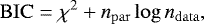 (30)
(30)
where 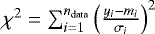 with yi is ith data point, mi the ith model point and σi the error bar of th ith data point. The values of the BIC and χ2 for each target are displayed on Fig. E.1. To compare the models, we have selected the model with the lowest BIC. However, the differences between the BIC values for a given dataset can be small and several models can be considered. Usually, models with a difference of more than 10 with the BIC of the best model can be ruled out whereas a difference between six and ten can be considered as moderately strong evidence for the best model, between two and six as positive evidence in favour of the best model and less than two as weak evidence (e.g., Aerts et al. 2018).
4 Results
In this section we present a first analysis of the fit results by discussing the important and most reliable parameters related to the ring morphology such as the near-IR sizes, the temperatures or the fluxes of the different components. We focus on the circumbinary environments in our comparison with YSOs.
4.1 Results of the model selection
For HD 93662, IRAS 19125+0343, IW Car and R Sct one model has very strong evidence over all the other models (ΔBIC > 10 for any other model). For all other targets, the most likely models are presented on Tables F.1–F.18. Five targets have the most likely model to have at least strong evidence (6 < ΔBIC < 10) over other models (AI Sco, HD 108015, HD 213985, IRAS 05208-2035, IRAS 17038-4815). Most of the likely models have similar parameters (i.e. within the error bars). In the rest of our analysis we use the most likely model (i.e. the model with the lowest BIC value).
The best-fit parameters are presented in Table A.1. As an estimation of the fit quality, the reduced χ2 ( = χ2 ∕ndata) values ranges from 0.5 to 6.6. The number of targets per model is displayed in the top panel of Fig. 3. Out of the sixteen models eleven were selected. For one target the simplest model was preferred (AC Her, #1). For three targets a binary model was preferred with no ring (HD93662 (#4), PS Gem (#18), and RU Cen (#20)). For ten targets models of a single star with a ring was selected while for ten targets a model with a binary surrounded by a ring was preferred. For twelve targets models with a binary were preferred and for nineteen targets models with a ring were preferred (their images are displayed in Fig. C.1).
In the bottom panel of Fig. 3 we can see how many models there are per number of parameters. Models with six or less parameters are not fitting the data well enough (apart for AC Her, #1). Thirteen targets (~55%) were fitted by models with thirteen parameters or more. This shows the complexity of the resolved structures.
The case of AC Her (#1) is interesting as it was previously observed in mid-IR with the MIDI instrument at the VLTI (Hillen et al. 2015). A disk with an inner rim at 68 au was fitted to the data, which corresponds to 42 mas. A rim of this size would be over-resolved by our observations, which is compatible with the most likely model: a star + an over-resolved flux. For the target with the richest dataset, IRAS 08544-4431 (#10), the most likely model corresponds to the model which was fitted in Hillen et al. (2016). The best-fit parameters are also very similar except the ring temperature Tring. This is due to the way the photosphereric spectrum is represented as in Hillen et al. (2016) it is assumed to be in the Rayleigh-Jeans regime (Fλ∝ λ−4) and here we use the fit to the photometry.
Matrix of parameters used in the different models.
Allowed parameter ranges.
 |
Fig. 3 Statistics of model selection. Top: number of targets per model. Bottom: number of targets per number of parameter of the selected model (complexity). |
4.2 Innerrim radius ruled by dust sublimation physics
For protoplanetary disks the size of the near-IR extended emission (the physical radius in au: a) correlates with the square root of the stellar luminosity (Lbol; Monnier & Millan-Gabet 2002; Lazareff et al. 2017) such as:
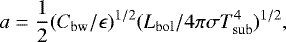 (31)
(31)
where Tsub is the sublimation temperature, Cbw is the backwarming coefficient (Kama et al. 2009), ϵ = Qabs(Tsub)∕Qabs(T*) is the dust grain cooling efficiency which is the ratio of Planck-averaged absorption cross-sections at the dust sublimation and stellar temperatures and σ the Stefan-Boltzmann constant. To study the size of the inner rim we use here and in the rest of the paper the half of the fitted ring diameter (θ) as it was done in studies of disks around YSOs (e.g., Monnier & Millan-Gabet 2002; Monnier et al. 2005; Lazareff et al. 2017). The rings having a given width (δθ) it is possible that the inner disk edge, usually defined by the location where the optical depth τ equals unity (e.g., Kama et al. 2009), can be closer than the ring radius. In Fig. 4 we plot the sizes of the ring models versus the central luminosity for pAGB binaries of our sample with, for reference, lines indicating theoretical sublimation radii for Tsub = 1000 K and 1500 K with Cbw = 1 and ϵ = 1. In order to compute the luminosities and the physical sizes of our targets we have used the Gaia parallaxes (Bailer-Jones et al. 2018). However, as our targets are binaries with a semi-amplitude that can be on the order of the parallax, those distances are likely biased by the orbital movement of the binary. Luckily, however, this does not impact the size luminosity diagram as both the physical size and the square root of the luminosity scale linearly with distance. An error on the distance will therefore displace a point along the size-luminosity relation.
Sizes of near-IR emission around pAGB binaries seem to scale with the stellar luminosity as it is the case for young stellar objects. However, the sizes of pAGB circumstellar emissions are systemically always offset toward sizes larger than for circumstellar emission around YSOs. This can be deduced more clearly from the histogram on Fig. 5.
There are three outliers (IRAS 10174-5704 (#11), R Sct (#19) and V494Vel (#23)) with very small sizes compared to their luminosity. Those three stars have also a large temperature for their environment (higher than 7000 K) meaning that the traced circumstellar environment is not thermal emission from dust.
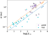 |
Fig. 4 Size-luminosity relation. The sizes are in log-scale. Purple points are pAGB binaries from this work. Purple open circles are pAGB binaries with Tring > 7000 K. Light blue points are Herbig Ae/Be stars from Lazareff et al. (2017). The blue and orange resp. dashed lines are the theoretical sublimation radius for Tsub = 1500 K and Tsub = 1000 K resp. |
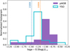 |
Fig. 5 Histogram of sizes scaled by square root of luminosity for pAGBs and YSOs. |
4.3 Dust temperature
The spectral channels of PIONIER allow us to probe the difference in spectral index between the central star and its environment. This is done by fitting the difference of level of the squared visibilities between the different channels. For a target in which such a difference is present, the fraction of the total flux that is resolved by the interferometer at any given baseline depends on the wavelength, hence the observed squared visibilities as well. This is called the chromatic effect. When there is a large difference in temperature between a central unresolved source and its resolved environment, the squared visibility increases with shorter wavelength for a given baseline (see Fig. 6).
We assumed the central star to have a given spectrum that we fit from photometry. The ring models assume a black-body emission for the ring. As we fix the primary spectrum to be what we fit from the photometry the difference inthe levels of the squared visibilities per channel will be reproduced by a given ring temperature. This temperaturemay not be the exact temperature at that location due to optical depth effects, but it gives a good first indication.
In Fig. 7 we show the histogram of temperatures we found for our models. On the one hand, two-third of the targets (13/19) have a low circumstellar emission temperature (Tring < 1600 K), equal or lower than the classical silicate sublimation temperatures we expect (~1500 K) indicating that the thermal emission of the inner rim of the disk dominates. The slightly lower temperatures agree with the shift toward larger sizes we see in the size-luminosity diagram for the pAGB with respect to YSOs. On the other hand, four targets have a circumstellar emission with a temperature of more than 7000 K: IRAS 05208-2035 (#9), IRAS 10174-5704 (#11), R Sct (#19), and V 494 Vel (#23). Three of them are also outliers in the size-luminosity diagram (see Sect. 4.2) pointing toward another origin of the circumstellar flux. For IRAS 05208-2035 (#9), the high-stellar-to-total flux ratio (90.5 ± 0.3%) makes this target special. The ring flux is perhaps stellar scattered light coming from the inner rim of the disk. Finally, between these two categories of temperatures, two targets have a temperature around 3000–4000 K (IRAS 17038-4815 (#13) and U Mon (#22)). Interestingly, those targets are expected to have pulsation with the largest amplitude (Δmag = 1.5 and 1.1 for IRAS 17038-4815 (#13) and U Mon (#22) resp.) among our sample. However, our data is too sparse to look for morphological changes induced by pulsations in these targets within the observations that span a large part of the pulsation cycle. Our models are able to reproduce the data reasonable without including any intrinsic variations.
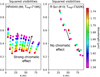 |
Fig. 6 Illustration of chromatic effect (see main text). Left: squared visibilities of HR4049 (#8) showing a strong chromatic effect. Right: squared visibilities for R Sct (#19) not showing such an effect. |
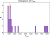 |
Fig. 7 Histogram of ring temperatures. |
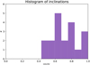 |
Fig. 8 Histogram of cosines of fitted inclinations. |
4.4 Disk inclinations
We can investigate the morphology of the circumbinary environment by looking at the ring inclinations. As our targets are surrounded by disks, the distribution of the cosines of inclinations should be flat. However, for spherical shells for instance, there would be a pile-up of objects at cosinc ~ 1.
Figure 8 displays the histogram of the cosines of our ring inclinations. There is clearly no pile-up at cos inc = 1. We see a rather flat distribution with a cut-off at about cosinc ~ 0.5 that corresponds to a inclination of ~60°. This is likely due to observational bias as the disks that are edge-on will absorb the visible light from the central stars. The cut-off of disk inclinations could therefore be a proxy to the characteristic thickness of the disk. The cut-off we see would translate to a disk thickness of h∕r ~0.8. However, there could be a model bias as at very high inclinations the model might not be able to reproduce the intensity distribution correctly.
4.5 Disk width
We are sensitive to the width of the emission coming from the disk. The parameter δθ measures the width of the ring in the units of the ring radius. In Fig. 9 we see this ring width parameter plotted against the size of the ring divided by the angular resolution of the largest baseline. We see that as long as the ring is resolved by the observations ( ) its width is better constrained and is below unity. It means that the circumbinary dust emission is compatible with a ring and not with an emission without a cavity (δθ ≥ 2) and that the ring has a significant radial width (δθ between 0.5 and 1).
4.6 Rim brightness distribution
All the models with a ring require at least a first order modulation. For a modulation due to the inclination of an optically and geometrically thick inner rim we will have a larger illumination in the direction of the minor axis (e.g., Isella & Natta 2005). If this is the case most of the targets would have a larger absolute value of the s1 coefficient and an almost zero value for c1. Figure 10 shows that this is not the case. The values for c1 and s1 are scattered. Inclination effects would produce more points with s1 sininc between 0 and 1 and c1 sininc between 0 and 0.3 (Lazareff et al. 2017). There is no clear evidence that the inclination is the main cause of the observed modulation.
Half of the targets prefer the second order modulation, also indicating that the inner rims are not ruled only by inclination effects but also by interactions with the inner binary and/or disk instabilities.
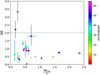 |
Fig. 9 Relative ring width (δθ) against degree of resolution of the ring. The colors indicate the ring inclination. The horizontal line indicates where the ring has no inner cavity (δθ ≥2). |
 |
Fig. 10 Direction of maximum of first order modulation. The dashed line represent the limit for inclination-like modulations (see text; Lazareff et al. 2017). The circle represent the maximum values for the modulation coefficients c1 and s1. |
4.7 Extended flux statistics
In IRAS 08544-4431 (#10), our best studied object, ~15% of the H-band flux is coming from an over-resolved emission (Hillen et al. 2016). Only half of this flux was accounted for by the radiative transfer model including a disk in hydrostatic equilibrium and scattered light (Kluska et al. 2018). The origin of this extended flux is not clear so far. This extended flux is easy to detect as it can be measured as the drop of visibility at short baselines. Figure 11 shows the ratio of the over-resolved (fbg) over the total non-stellar flux (fcircum = 1-fprim-fsec). IRAS 08544-4431 (#10) has ~42% of its non-stellar flux to be over-resolved. 14 out of 19 targets (~75%) have this ratio larger than 10% and three of them have it around 50%.
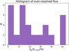 |
Fig. 11 Histogram of fractions of over-resolved non-stellar flux. |
5 Discussion
In this section we will discuss the results and interpret them in an extended context. We will first discuss the outliers in Sect. 5.1. We then discuss the shift between pAGB and YSOs in the size luminosity relation (Sect. 5.2). Then we will discuss the relation between disk inclination and the RVb phenomenon (variable extinction or scattering in the line of sight during orbital motion; Sect. 5.3). We will discuss the radial structure of the disk by comparing the size of the emission in the near-IR with the one in the mid-IR (Sect 5.4). Finally, in Sect. 5.5, we will discuss the differences and similarities with the disks around YSOs.
5.1 Outliers
Four targets from our sample are outliers in the fact that the temperature of their environment is very high (Tring > 7000 K), significantly above any dust sublimation temperature. Here we summarize results published in literature and give an interpretation of the origin of their pecularities.
5.1.1 IRAS 05208-2035 (#9)
This source is an outlier in de Ruyter et al. (2006): its IR excess starts at longer wavelengths (after L-band).
This visibilities show a reversed chromatic effect that is the squared visibility decreases with decreasing wavelengths. It happens when the environment is bluer than the emission from the central source Our models are not able to reproduce this effect. This effect can be produced by stellar light scattered on the disk surface.
5.1.2 IRAS 10174-5704 (#11)
This source has a high temperature for its environment and a small radius. It was included in the mid-IR interferometric survey of post-AGB binaries with MIDI (Hillen et al. 2017). In this sample it is standing out because of its large size. Also in the Spitzer survey of Gielen et al. (2011) it was noticed that the spectrum of this source is dominated by amorphous silicates with no crystalline dust features. It was postulated in the latter that IRAS 10174-5704 is likely a luminous super-giant. It would explain why this source is an outlier in our survey as well.
5.1.3 R Sct (#19)
R Sct is one of the only pAGB targets for which a surface magnetic field was detected (Sabin et al. 2015). It is also classified as “uncertain” by Gezer et al. (2015), on the basis of its WISE photometric colors. Its binary nature is not confirmed and the SED shows a very minimal IR excess that is more reminiscent of an outflow than of a disk.
5.1.4 V 494 Vel (#23)
This target shows photometric fluctuations but without any periodicity (Kiss et al. 2007). As for R Sct, the binarity nature of this source is uncertain. We note that the target is usually referred in previous studies as IRAS 09400-4733 (Kwok et al. 1997; de Ruyter et al. 2006; Kiss et al. 2007; Szczerba et al. 2007).
5.2 Origin of the shift between pAGBs and YSOs in the size luminosity relation
There can be two explanations for the systematic offset between inner rim sizes (scaled to the squared stellar luminosity, see Fig. 5) between pAGB and YSO sources. The two explanations are about factors that influence the dust sublimation radius.
A first factor that could be different between pAGBs and YSOs is the dust type. For a given gas density, different types of dust will have different sublimation temperatures. For example silicates, that are Oxygen rich, will have lower dust sublimation temperaturethan Carbon-rich dust (e.g., Kobayashi et al. 2011). Carbon-rich dust is more abundant in PPDs than in disks around pAGB (e.g., Gielen et al. 2011). Although amorphous C does not show significant spectral features, the absence of distinct features from other C-rich dust species in the mid-IR spectra indicates a low abundance of C in the pAGB circumbinary dust. Mg-rich species like Olivine on the other hand are abundantly present (Gielen et al. 2008, 2011; Hillen et al. 2015). Therefore, in pAGB the overall dust sublimation temperature will be higher and the inner disk radius will be larger as observed.
Another factor is the local gas density. Assuming the same dust species, the same temperature will be reached farther away from the central star in the pAGBs because of higher luminosity of the central star than in YSOs. Assuming the same central stellar masses, same disk masses and a similar disk structure for the two types of objects, that is a decreasing surface density with radius, the local density will be lower at those locations in pAGBs (also because of weaker gravity due to the central star). As the dust sublimation temperature depends on the gas density (e.g., Kama et al. 2009), it will be lower for pAGBs and hence the inner dust rim will be larger.
We can compare the measured interferometric temperatures of the near-IR circumbinary emission of pAGBs to those of the environmentof YSOs. Figure 12 shows that pAGBs have systemically lower measured disk rim temperatures than YSOs.
One could expect that some targets will show larger sizes that the theoretical dust sublimation radius because of the dynamical interaction between the inner binary and the disk. This interaction would push the disk rim at a radius ~1.7 times larger than the binary separation (Artymowicz & Lubow 1994). This would have been seen by having some targets higher up in the size-luminosity diagram (Fig. 4) and that some ring diameters (Θ) would be on the order of 1.7× the binary separation which we do not see (Fig. 13). Therefore, the dust component is no tracing the disk dynamical truncation by the inner binary.
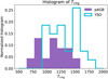 |
Fig. 12 Histogram of temperatures of near-IR circumbinary emission for objects having Tring between 500and 2000 K. pAGBa are in purple and YSOs from Lazareff et al. (2017) are in blue. |
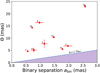 |
Fig. 13 Comparison between ring diameter (Θ) and binary separation ( |
5.3 Relation between the RVb phenomenon and disk inclination
The RV Tauri stars are variable pulsating post-AGB stars (e.g., Kiss et al. 2007; Kiss & Bódi 2017; Manick et al. 2017). They display alternate deep and shallow minima. A sub-sample of these stars has a long-period variation of the mean luminosity (Pollard et al. 1996) and are classified as RVb. More generally this long-period photometric variation is observed in non RV Tauri stars as welland is caused by variable extinction or scattering in the line of sight due to orbital motion of the central binary (Kiss et al. 2007). It is interpreted as caused by a highly inclined disk shadowing the primary at certain phases of the orbit (Van Winckel et al. 1999; Manick et al. 2017). As we are sensitive to the disk inclination we can test this hypothesis.
In our sample, there are nine targets displaying the RVb phenomenon: AI Sco (#2), HD 95767(#5), HD 213985 (#7), HR 4049(#8), IRAS 19125+0343 (#15), IW Car (#16), SX Cen(#21), U Mon (#22), and V 494 Vel (#23) (Waelkens et al. 1991; Waelkens & Waters 1995; Kiss et al. 2007; Kiss & Bódi 2017). While HD 213985 (#7), SX Cen (#21), and U Mon (#22) are the most inclined disks from this survey (inc ~ 60°) confirming the inclined disk hypothesis, the other objects are only moderately inclined implying very high disk scale-height for the disk shadowing interpretation to be true. The histogram of inclinations for all sources and RVb sources shows that most of the RVb sources have the highest inclination (Fig. 14). One RVb source is found to have a pole-on inclination: HD 95767 (#5). The other likely model for this source also point toward a pole-on orientation (Fig. F.4). We also note that three sources have high inclinations (above 50°) without showing the RVb phenomenon: EN TrA (#3), IRAS 05208-2035 (#9), and IRAS 15469-5311 (#12). The apparent inclinations are deduced from an aspect ratio and, given the poor uv-coverage for some sources, need to be confirmed by further studies.
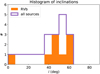 |
Fig. 14 Histogram of inclinations for objects from our sample showing RVb phenomenon (orange) and the whole sample (purple). |
5.4 Comparison between near-IR and mid-IR sizes
We see in Sect. 4.2 that the size of the near-IR emission is ruled by dust sublimation physics as it is proportional to the square root luminosity of the central star. However the structure of the disk can be constrained if it is observed at different wavelengths. To do so we can compare the diameters of the circumstellar emission at the mid-IR probed by MIDI at 10 μm (Hillen et al. 2016)with the diameters from this work. The two diameters are plotted against each other on Fig. 15. There is a relation of proportionality where θMIR ≈ 2θNIR.
Most of the models of protoplanetary disks predict a power-law for the radial temperature dependence T ∝r−α (e.g., Lynden-Bell & Pringle 1974; Kenyon & Hartmann 1987). In several studies the used power-law index is either α = 0.5 or α = 0.75 (e.g., Kraus et al. 2008). Assuming that the disk emits as a black-body with a power-law radial temperature profile and that the inner disk radius has a temperature of 1100 K (see Sect. 4.3) we can simulate the radial profile of the emission in both the near and mid-IR. From those profiles we can take the ratio of the half-light diameters (Θ) between the near-IR and the mid-IR. Those ratios are reported in Fig. 15. We can see that most of our targets fall within the two limits set by the two temperature power-laws. This points toward disks that have a similar radial temperature dependence and a smooth radial disk structure in the inner disk regions (<30 au).
There are some sources that are standing out from this picture. IRAS 10174-5704 (#11) has a mid-IR size (2hlr=150±8mas; Hillen et al. 2017) ~115 times larger than the near-IR size from this work. U Mon (#22) has also a relatively large mid to near IR size ratio. This target is showing the RVb phenomenon and has a very complex visibility profile that could only be reproduced by the most complex model. The result of the fit is displaying a strong azimuthal modulation showing a complex morphology of this target. Finally IW Car (#16) is the only outlier having a significantly small mid to near-IR size ratio. This target is showing an RVb phenomenon as well, however, we find a moderate inclination in our work. It is fitted by the most complex model and has still a relatively large  = 3.9. It is possible that the models are not able to reproduce all the complexity of that source and that it could have an effect on the derived size. More observations of this target are therefore needed to confirm its status.
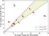 |
Fig. 15 Comparison between MIDI half light diameters and PIONIER diameters for ring like targets. The dashed lines represent the models of disks with a temperature dependence that scales with a power-law of the radius. IRAS 10174-5704 (#11) is outside the limits of this plot (see Sect. 5.4) and is not appearing for clarity reasons. |
5.5 Continuing the comparison between pAGB and YSOs
Despite a completely different formation process, disks surrounding post-AGB binaries and those surrounding young stars are similar with respect to several criteria. They are often compared to young intermediate mass Herbig stars. The disks around Herbig Ae/Be stars are classified into two groups (Meeus et al. 2001; Maaskant et al. 2013; Menu et al. 2015): disks with flared or gapped structure (group I) and flat disks (group II). It was advocated that disks around post-AGB binaries are group II sources (de Ruyter et al. 2006; Hillen et al. 2017) because of their SED and mid-IR sizes and colors.
In this work we push the comparison further. We recall and discuss here the main points of comparison between those two kinds of disks arising from this study.
The near-IR size-luminosity relation
We show in Sect. 4.2 that the relation extends for the near-IR emission around post-AGB disks. As these targets have a higher luminosity than most of the young intermediate mass Herbig Ae/Be stars, we are able to probe very high luminosity regimes. This result shows that the near-IR emission in post-AGB is also mainly ruled by dust sublimation rather than dynamical disk truncation by the inner binary. However, the shift toward larger sizes and the ring temperatures, Tring, inform us on different properties of the disks around post-AGB binaries that lowers the temperature of their dust sublimation front. We postulate that it can be due to smaller local gas density or different dust grain mineralogy or both.
Amount of extended flux
For Herbig Ae/Be stars, the disks that have a double-peaked SED in the mid-IR (group I; Meeus et al. 2001) display an over-resolved-to-non-stellar flux ratio larger than 5% whereas the targets with a flat SED in the mid-IR (group II) have this flux ratio lower than 5% (Lazareff et al. 2017). In our sample, fourteen targets have more than 10% of non-stellar flux to be over-resolved. This ratio can reach 50% in some cases. This confirms that there is a significant contribution from an over-resolved flux in the near-IR for these targets. It is the first time we observe a specific feature of group I Herbig disks in pAGB disks. The origin of this extended flux (fbg0) is unknown and should be the focus of future studies. It can be related to the disk structure (e.g., disk flaring, presence of a gap) or to a mechanism lifting the dust from the disk (e.g., disk wind, jet from the secondary).
6 Conclusions
We summarize here the most important findings of our interferometric survey. Despite the very inhomogeneous (u, v)-coverages obtained we can conclude that:
- 1.
For most of the sources 19/23 a compact but resolved ring-like H-band emissioncomponent is detected which confirms the presence of a disk in pAGB binaries.
- 2.
Most of the targets (14/23) prefer models with more than ten parameters and several targets (6/23) prefer the most complex models with fifteen or more, including complex azimuthal modulations, even with a limited (u, v)-plane coverage.
- 3.
There is a relation of proportionality between the size of the near-IR circumstellar emission and the square root of the stellar luminosity as it is the case around YSOs, suggesting that the near-IR extended emission is also linked to the dust sublimation region around pAGBs.
- 4.
The measured temperature of the near-IR circumbinary emission is lower (median ring temperature of ~1200–1300 K) for pAGB disks and the sizes of the near-IR circumstellar emission are systematically a bit larger than for YSOs. This canbe due to different dust grain mineralogy and/or lower gas density at the sublimation front.
- 5.
The dust sublimation front has width-to-radius ratios spanning between 0.5 and unity.
- 6.
A significant fraction of the near-IR emission is over-resolved by our observations. This ratio is higher than for Herbig Ae/Be stars. The origin of this circumstellar flux is unknown.
Given the complexity of our targets and the limitations of geometrical modeling of the near-IR interferometric observables, we believe that a time series of interferometric images is the only way to come to a sharp view on the physics that drives the interactions in the inner regions of these objects. The presented survey (see Fig. C.1) and our imaging campaign of IRAS 08544-4431 (Hillen et al. 2016; Kluska et al. 2018) have demonstrated the potential of near-IR interferometric images, have shown which targets can be well resolved with the existing instrumentation and which are most interesting for follow-up campaigns.
The focus of this paper has been mostly on the circumbinary emission, as this is most reliably detected in our data. Our survey also demonstrates, however, that there is a lot of potential for detecting the companions, even if the here presented detections are likely not free of model bias. Model-independent determinations of the binary orbits will require significant investments of observing time though, as significantly better uv-coverages are required (like that of IRAS 08544-4431), and this at various orbital phases.
To investigate the origin of the over-resolved flux (outflow, disk wind, disk structure), direct imaging in scattered light should bring strong constraints. Finally, a complete view of the dust disk structure such as millimeter observations with ALMA will allow us to investigate the possibility of second-generation planet formation in these disks.
Acknowledgements
We thank the referee for his comments that improved the clarity of the paper. J.K. and H.V.W. acknowledge support from the research council of the KU Leuven under grant number C14/17/082. D.K. acknowledges support from Australian Research Council DECRA grant DE190100813. This research has made use of the Jean-Marie Mariotti Center Aspro service3. We used the following internet-based resources: NASA Astrophysics Data System for bibliographic services; Simbad; the VizieR online catalogs operated by CDS.
Appendix A Best-fit parameters
Best-fit parameters.
Observation log.
Appendix B Interferometric dataset
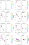 |
Fig. B.1 Squared visibilities and closure phases for each target. The color represent the wavelength. |
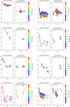 |
Fig. B.1 continued. |
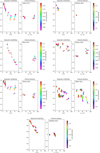 |
Fig. B.1 continued. |
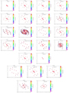 |
Fig. B.2 (u, v)-plane for each target. |
Appendix C Images of the targets where the most likely model has a disk
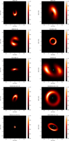 |
Fig. C.1 Best fit model images. The green star represents the primary. The cyan star represents the secondary. |
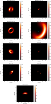 |
Fig. C.1 continued. |
Appendix D Best-fit model comparison to the data
 |
Fig. D.1 Best fit model (blue) versus data (black) for squared visibilities and closure phases for each target. Top panels are the data and the bottom panels are the residuals in σ. |
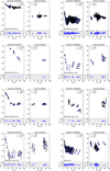 |
Fig. D.1 continued. |
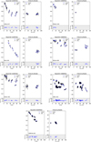 |
Fig. D.1 continued. |
Appendix E The BICand χ2 evolution per model for each target
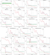 |
Fig. E.1 BICand χ2 per model for each target. |
Appendix F Most likely models for each target as determined with the BIC
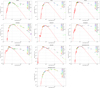 |
Fig. F.1 Spectral energy distributions of the targets of our survey for which no SED was already published. |
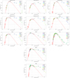 |
Fig. F.1 continued. |
Best-fit parameters of the selected models for AC Her (#1).
Best-fit parameters of the selected models for AI Sco.
Best-fit parameters of the selected models for EN TrA.
Best-fit parameters of the selected models for HD 95767.
Best-fit parameters of the selected models for HD 108015.
Best-fit parameters of the selected models for HD 213985.
Best-fit parameters of the selected models for HR 4049.
Best-fit parameters of the selected models for IRAS 05208-2035.
Best-fit parameters of the selected models for IRAS 08544-4431.
Best-fit parameters of the selected models for IRAS 10174-5704.
Best-fit parameters of the selected models for IRAS 15469-5311.
Best-fit parameters of the selected models for IRAS 17038-4815.
Best-fit parameters of the selected models for IRAS 18123+0511.
Best-fit parameters of the selected models for LR Sco.
Best-fit parameters of the selected models for PS Gem.
Best-fit parameters of the selected models for SX Cen.
Best-fit parameters of the selected models for U Mon.
Best-fit parameters of the selected models for V494 Vel.
SED best fit parameters.
References
- Aerts, C., Molenberghs, G., Michielsen, M., et al. 2018, ApJS, 237, 15 [NASA ADS] [CrossRef] [Google Scholar]
- Anderson, E., & Francis, C. 2012, VizieR Online Data Catalog: V/137B [Google Scholar]
- Artymowicz, P., & Lubow, S. H. 1994, ApJ, 421, 651 [NASA ADS] [CrossRef] [Google Scholar]
- Bailer-Jones, C. A. L., Rybizki, J., Fouesneau, M., Mantelet, G., & Andrae, R. 2018, VizieR Online Data Catalog: I/347 [Google Scholar]
- Bollen, D., Van Winckel, H., & Kamath, D. 2017, A&A, 607, A60 [NASA ADS] [CrossRef] [EDP Sciences] [Google Scholar]
- Bujarrabal, V., Alcolea, J., Van Winckel, H., Santander-García, M., & Castro-Carrizo, A. 2013, A&A, 557, A104 [NASA ADS] [CrossRef] [EDP Sciences] [Google Scholar]
- Bujarrabal, V., Castro-Carrizo, A., Alcolea, J., & Van Winckel, H. 2015, A&A, 575, L7 [NASA ADS] [CrossRef] [EDP Sciences] [Google Scholar]
- Bujarrabal, V., Castro-Carrizo, A., Alcolea, J., et al. 2016, A&A, 593, A92 [NASA ADS] [CrossRef] [EDP Sciences] [Google Scholar]
- Bujarrabal, V., Castro-Carrizo, A., Alcolea, J., et al. 2017, A&A, 597, L5 [NASA ADS] [CrossRef] [EDP Sciences] [Google Scholar]
- Bujarrabal, V., Castro-Carrizo, A., Winckel, H. V., et al. 2018, A&A, 614, A58 [NASA ADS] [CrossRef] [EDP Sciences] [Google Scholar]
- Cutri, R. M., Skrutskie, M. F., van Dyk, S., et al. 2003, VizieR Online Data Catalog: II/246 [Google Scholar]
- Cutri, R. M., Wright, E. L., Conrow, T., et al. 2012, VizieR Online Data Catalog: II/311 [Google Scholar]
- de Ruyter, S., Van Winckel, H., Maas, T., et al. 2006, A&A, 448, 641 [NASA ADS] [CrossRef] [EDP Sciences] [Google Scholar]
- Degroote, P., Briquet, M., Catala, C., et al. 2009, A&A, 506, 111 [NASA ADS] [CrossRef] [EDP Sciences] [Google Scholar]
- Dermine, T., Izzard, R. G., Jorissen, A., & Van Winckel, H. 2013, A&A, 551, A50 [NASA ADS] [CrossRef] [EDP Sciences] [Google Scholar]
- Dominik, C., Dullemond, C. P., Cami, J., & van Winckel, H. 2003, A&A, 397, 595 [NASA ADS] [CrossRef] [EDP Sciences] [Google Scholar]
- Ducati, J. R. 2002, VizieR Online Data Catalog: II/237 [Google Scholar]
- Duchêne, G., & Kraus, A. 2013, Ann. Rev. Astron. Astrophys., 51, 269 [CrossRef] [Google Scholar]
- Egan, M. P., Price, S. D., Kraemer, K. E., et al. 2003, VizieR Online Data Catalog: V/114 [Google Scholar]
- Foreman-Mackey, D., Hogg, D. W., Lang, D., & Goodman, J. 2013, PASP, 125, 306 [CrossRef] [Google Scholar]
- Fortin, F.-A., De Rainville, F.-M., Gardner, M.-A., Parizeau, M., & Gagné, C. 2012, J. Mach. Learn. Res., 13, 2171 [Google Scholar]
- Gaia Collaboration 2016, VizieR Online Data Catalog: I/337 [Google Scholar]
- Gezer, I., Van Winckel, H., Bozkurt, Z., et al. 2015, MNRAS, 453, 133 [NASA ADS] [CrossRef] [Google Scholar]
- Gielen, C., Van Winckel, H., Min, M., Waters, L. B. F. M., & Lloyd Evans, T. 2008, A&A, 490, 725 [NASA ADS] [CrossRef] [EDP Sciences] [Google Scholar]
- Gielen, C., Bouwman, J., Van Winckel, H., et al. 2011, A&A, 533, A99 [NASA ADS] [CrossRef] [EDP Sciences] [Google Scholar]
- Giridhar, S., Rao, N. K., & Lambert, D. L. 1994, ApJ, 437, 476 [NASA ADS] [CrossRef] [Google Scholar]
- Giridhar, S., Lambert, D. L., & Gonzalez, G. 2000, ApJ, 531, 521 [NASA ADS] [CrossRef] [Google Scholar]
- Gorlova, N., Van Winckel, H., Ikonnikova, N. P., et al. 2015, MNRAS, 451, 2462 [NASA ADS] [CrossRef] [Google Scholar]
- Hardy, A., Schreiber, M. R., Parsons, S. G., et al. 2016, MNRAS, 459, 4518 [NASA ADS] [CrossRef] [Google Scholar]
- Hauck, B., & Mermilliod, M. 1998, A&AS, 129, 431 [NASA ADS] [CrossRef] [EDP Sciences] [Google Scholar]
- Helou, G., & Walker, D. W. 1988, NASA RP-1190, 7, 0 [Google Scholar]
- Henden, A. A., Templeton, M., Terrell, D., et al. 2016, VizieR Online Data Catalog: II/336 [Google Scholar]
- Hillen, M., Menu, J., Van Winckel, H., et al. 2014, A&A, 568, A12 [NASA ADS] [CrossRef] [EDP Sciences] [Google Scholar]
- Hillen, M., de Vries, B. L., Menu, J., et al. 2015, A&A, 578, A40 [NASA ADS] [CrossRef] [EDP Sciences] [Google Scholar]
- Hillen, M., Kluska, J., Le Bouquin, J.-B., et al. 2016, A&A, 588, L1 [NASA ADS] [CrossRef] [EDP Sciences] [Google Scholar]
- Hillen, M., Van Winckel, H., Menu, J., et al. 2017, A&A, 599, A41 [NASA ADS] [CrossRef] [EDP Sciences] [Google Scholar]
- Hoeg, E., Bässgen, G., Bastian, U., et al. 1997, A&A, 323, L57 [NASA ADS] [Google Scholar]
- Høg, E., Fabricius, C., Makarov, V. V., et al. 2000, A&A, 355, L27 [Google Scholar]
- Isella, A., & Natta, A. 2005, A&A, 438, 899 [NASA ADS] [CrossRef] [EDP Sciences] [Google Scholar]
- Ishihara, D., Onaka, T., Kataza, H., et al. 2010, A&A, 514, A1 [NASA ADS] [CrossRef] [EDP Sciences] [Google Scholar]
- Johnson, H. L., & Mitchell, R. I. 1975, Rev. Mex. Astron. Astrofis., 1, 299 [Google Scholar]
- Johnson, H. L., Mitchell, R. I., Iriarte, B., & Wisniewski, W. Z. 1966, Commun. Lunar Planet. Lab., 4, 99 [NASA ADS] [Google Scholar]
- Kama, M., Min, M., & Dominik, C. 2009, A&A, 506, 1199 [NASA ADS] [CrossRef] [EDP Sciences] [Google Scholar]
- Kamath, D., & Van Winckel, H. 2019, MNRAS, 486, 3524 [NASA ADS] [CrossRef] [Google Scholar]
- Kashi, A., & Soker, N. 2018, MNRAS, 480, 3195 [NASA ADS] [Google Scholar]
- Kenyon, S. J., & Hartmann, L. 1987, ApJ, 323, 714 [NASA ADS] [CrossRef] [Google Scholar]
- Kharchenko, N. V. 2001, Kinematika i Fizika Nebesnykh Tel, 17, 409 [NASA ADS] [Google Scholar]
- Kiss, L. L., & Bódi, A. 2017, A&A, 608, A99 [NASA ADS] [CrossRef] [EDP Sciences] [Google Scholar]
- Kiss, L. L., Derekas, A., Szabó, G. M., Bedding, T. R., & Szabados, L. 2007, MNRAS, 375, 1338 [NASA ADS] [CrossRef] [Google Scholar]
- Kluska, J., Hillen, M., Van Winckel, H., et al. 2018, A&A, 616, A153 [NASA ADS] [CrossRef] [EDP Sciences] [Google Scholar]
- Kobayashi, H., Kimura, H., Watanabe, S. i., Yamamoto, T., & Müller, S. 2011, Earth, Planets, and Space, 63, 1067 [NASA ADS] [CrossRef] [Google Scholar]
- Kraus, S., Preibisch, T., & Ohnaka, K. 2008, ApJ, 676, 490 [NASA ADS] [CrossRef] [Google Scholar]
- Kurucz, R. L. 1993, VizieR Online Data Catalog: VI/39 [Google Scholar]
- Kwok, S., Volk, K., & Bidelman, W. P. 1997, ApJS, 112, 557 [NASA ADS] [CrossRef] [MathSciNet] [Google Scholar]
- Lasker, B. M., Lattanzi, M. G., McLean, B. J., et al. 2008, AJ, 136, 735 [NASA ADS] [CrossRef] [PubMed] [Google Scholar]
- Lazareff, B., Berger, J.-P., Kluska, J., et al. 2017, A&A, 599, A85 [NASA ADS] [CrossRef] [EDP Sciences] [Google Scholar]
- Le Bouquin, J.-B., Berger, J.-P., Lazareff, B., et al. 2011, A&A, 535, A67 [NASA ADS] [CrossRef] [EDP Sciences] [Google Scholar]
- Lynden-Bell, D., & Pringle, J. E. 1974, MNRAS, 168, 603 [NASA ADS] [CrossRef] [Google Scholar]
- Maas, T., Van Winckel, H., & Waelkens, C. 2002, A&A, 386, 504 [NASA ADS] [CrossRef] [EDP Sciences] [Google Scholar]
- Maas, T., Van Winckel, H., Lloyd Evans, T., et al. 2003, A&A, 405, 271 [NASA ADS] [CrossRef] [EDP Sciences] [Google Scholar]
- Maas, T., Van Winckel, H., & Lloyd Evans, T. 2005, A&A, 429, 297 [NASA ADS] [CrossRef] [EDP Sciences] [Google Scholar]
- Maaskant, K. M., Honda, M., Waters, L. B. F. M., et al. 2013, A&A, 555, A64 [NASA ADS] [CrossRef] [EDP Sciences] [Google Scholar]
- Manick, R., Van Winckel, H., Kamath, D., Hillen, M., & Escorza, A. 2017, A&A, 597, A129 [NASA ADS] [CrossRef] [EDP Sciences] [Google Scholar]
- Marsh, T. R., Parsons, S. G., Bours, M. C. P., et al. 2014, MNRAS, 437, 475 [NASA ADS] [CrossRef] [Google Scholar]
- Matrà, L., Wyatt, M. C., Wilner, D. J., et al. 2019, AJ, 157, 135 [NASA ADS] [CrossRef] [Google Scholar]
- Meeus, G., Waters, L. B. F. M., Bouwman, J., et al. 2001, A&A, 365, 476 [NASA ADS] [CrossRef] [EDP Sciences] [Google Scholar]
- Menu, J., van Boekel, R., Henning, T., et al. 2015, A&A, 581, A107 [NASA ADS] [CrossRef] [EDP Sciences] [Google Scholar]
- Mermilliod, J. C. 2006, VizieR Online Data Catalog: II/168 [Google Scholar]
- Mermilliod, J. C., Mermilliod, M., & Hauck, B. 1997, A&AS, 124, 349 [NASA ADS] [CrossRef] [EDP Sciences] [Google Scholar]
- Monnier, J. D., & Millan-Gabet, R. 2002, ApJ, 579, 694 [NASA ADS] [CrossRef] [Google Scholar]
- Monnier, J. D., Millan-Gabet, R., Billmeier, R., et al. 2005, ApJ, 624, 832 [NASA ADS] [CrossRef] [Google Scholar]
- Morel, M., & Magnenat, P. 1978, A&AS, 34, 477 [NASA ADS] [Google Scholar]
- Murakami, H., Baba, H., Barthel, P., et al. 2007, PASJ, 59, S369 [NASA ADS] [CrossRef] [MathSciNet] [Google Scholar]
- Nascimbeni, V., Piotto, G., Ortolani, S., et al. 2016, MNRAS, 463, 4210 [Google Scholar]
- Nie, J. D., Wood, P. R., & Nicholls, C. P. 2012, MNRAS, 423, 2764 [NASA ADS] [CrossRef] [Google Scholar]
- Ofek, E. O. 2008, PASP, 120, 1128 [NASA ADS] [CrossRef] [Google Scholar]
- Oomen, G.-M., Van Winckel, H., Pols, O., et al. 2018, A&A, 620, A85 [NASA ADS] [CrossRef] [EDP Sciences] [Google Scholar]
- Parsons, S. G., Marsh, T. R., Bours, M. C. P., et al. 2014, MNRAS, 438, L91 [NASA ADS] [CrossRef] [Google Scholar]
- Paunzen, E., Duffee, B., Heiter, U., Kuschnig, R., & Weiss, W. W. 2001, A&A, 373, 625 [NASA ADS] [CrossRef] [EDP Sciences] [Google Scholar]
- Pollard, K. R., Cottrell, P. L., Kilmartin, P. M., & Gilmore, A. C. 1996, MNRAS, 279, 949 [NASA ADS] [Google Scholar]
- Rafikov, R. R. 2016, ApJ, 830, 8 [NASA ADS] [CrossRef] [Google Scholar]
- Richmond, M. W. 2007, PASP, 119, 1083 [NASA ADS] [CrossRef] [Google Scholar]
- Sabin, L., Wade, G. A., & Lèbre, A. 2015, MNRAS, 446, 1988 [NASA ADS] [CrossRef] [Google Scholar]
- Sahai, R., Claussen, M. J., Schnee, S., Morris, M. R., & Sánchez Contreras, C. 2011, ApJ, 739, L3 [NASA ADS] [CrossRef] [Google Scholar]
- Schleicher, D. R. G., & Dreizler, S. 2014, A&A, 563, A61 [NASA ADS] [CrossRef] [EDP Sciences] [Google Scholar]
- Schwarz, G. 1978, Ann. Stat., 6, 461 [Google Scholar]
- Shiber, S., Kashi, A., & Soker, N. 2017, MNRAS, 465, L54 [NASA ADS] [CrossRef] [Google Scholar]
- Spitzer Science, C. 2009, VizieR Online Data Catalog: II/293 [Google Scholar]
- Szczerba, R., Siódmiak, N., Stasińska, G., & Borkowski, J. 2007, A&A, 469, 799 [NASA ADS] [CrossRef] [EDP Sciences] [Google Scholar]
- Thomas, J. D., Witt, A. N., Aufdenberg, J. P., et al. 2013, MNRAS, 430, 1230 [NASA ADS] [CrossRef] [Google Scholar]
- Thun, D., Kley, W., & Picogna, G. 2017, A&A, 604, A102 [NASA ADS] [CrossRef] [EDP Sciences] [Google Scholar]
- Urban, S. E., Corbin, T. E., Wycoff, G. L., et al. 1998, AJ, 115, 1212 [NASA ADS] [CrossRef] [Google Scholar]
- Van Winckel, H. 1997, A&A, 319, 561 [NASA ADS] [Google Scholar]
- Van Winckel, H. 2003, ARA&A, 41, 391 [NASA ADS] [CrossRef] [Google Scholar]
- Van Winckel, H. 2018, ArXiv e-prints [arXiv:1809.00871] [Google Scholar]
- Van Winckel, H., Waelkens, C., Waters, L. B. F. M., et al. 1998, A&A, 336, L17 [NASA ADS] [Google Scholar]
- Van Winckel, H., Waelkens, C., Fernie, J. D., & Waters, L. B. F. M. 1999, A&A, 343, 202 [NASA ADS] [Google Scholar]
- Van Winckel, H., Lloyd Evans, T., Briquet, M., et al. 2009, A&A, 505, 1221 [NASA ADS] [CrossRef] [EDP Sciences] [Google Scholar]
- Völschow, M., Banerjee, R., & Hessman, F. V. 2014, A&A, 562, A19 [NASA ADS] [CrossRef] [EDP Sciences] [Google Scholar]
- Vos, J., Østensen, R. H., Marchant, P., & Van Winckel, H. 2015, A&A, 579, A49 [NASA ADS] [CrossRef] [EDP Sciences] [Google Scholar]
- Waelkens, C., Lamers, H. J. G. L. M., Waters, L. B. F. M., et al. 1991, A&A, 242, 433 [Google Scholar]
- Waelkens, C., & Waters, L. B. F. M. 1995, Ap&SS, 223, 202 [NASA ADS] [Google Scholar]
- Waters, L. B. F. M., Trams, N. R., & Waelkens, C. 1992, A&A, 262, L37 [NASA ADS] [Google Scholar]
Accessible at oidb.jmmc.fr
The used parameters to model for the photospheric flux are shown Table F.19.
Available at http://www.jmmc.fr/aspro
All Tables
All Figures
|
Fig. 1 Illustration of four azimuthal modulation coefficients on ring geometry. For each quadrant all modulation parameters are kept to zero apart from the one displayed. The red star shows the center of the ring. |
| In the text | |
|
Fig. 2 Tree of models. The single star and background models are in orange, the single star and a ring models are in blue, the binary models are in light green and the binary and ring models are in dark green. |
| In the text | |
|
Fig. 3 Statistics of model selection. Top: number of targets per model. Bottom: number of targets per number of parameter of the selected model (complexity). |
| In the text | |
|
Fig. 4 Size-luminosity relation. The sizes are in log-scale. Purple points are pAGB binaries from this work. Purple open circles are pAGB binaries with Tring > 7000 K. Light blue points are Herbig Ae/Be stars from Lazareff et al. (2017). The blue and orange resp. dashed lines are the theoretical sublimation radius for Tsub = 1500 K and Tsub = 1000 K resp. |
| In the text | |
|
Fig. 5 Histogram of sizes scaled by square root of luminosity for pAGBs and YSOs. |
| In the text | |
|
Fig. 6 Illustration of chromatic effect (see main text). Left: squared visibilities of HR4049 (#8) showing a strong chromatic effect. Right: squared visibilities for R Sct (#19) not showing such an effect. |
| In the text | |
|
Fig. 7 Histogram of ring temperatures. |
| In the text | |
|
Fig. 8 Histogram of cosines of fitted inclinations. |
| In the text | |
|
Fig. 9 Relative ring width (δθ) against degree of resolution of the ring. The colors indicate the ring inclination. The horizontal line indicates where the ring has no inner cavity (δθ ≥2). |
| In the text | |
|
Fig. 10 Direction of maximum of first order modulation. The dashed line represent the limit for inclination-like modulations (see text; Lazareff et al. 2017). The circle represent the maximum values for the modulation coefficients c1 and s1. |
| In the text | |
|
Fig. 11 Histogram of fractions of over-resolved non-stellar flux. |
| In the text | |
|
Fig. 12 Histogram of temperatures of near-IR circumbinary emission for objects having Tring between 500and 2000 K. pAGBa are in purple and YSOs from Lazareff et al. (2017) are in blue. |
| In the text | |
|
Fig. 13 Comparison between ring diameter (Θ) and binary separation ( |
| In the text | |
|
Fig. 14 Histogram of inclinations for objects from our sample showing RVb phenomenon (orange) and the whole sample (purple). |
| In the text | |
|
Fig. 15 Comparison between MIDI half light diameters and PIONIER diameters for ring like targets. The dashed lines represent the models of disks with a temperature dependence that scales with a power-law of the radius. IRAS 10174-5704 (#11) is outside the limits of this plot (see Sect. 5.4) and is not appearing for clarity reasons. |
| In the text | |
|
Fig. B.1 Squared visibilities and closure phases for each target. The color represent the wavelength. |
| In the text | |
|
Fig. B.1 continued. |
| In the text | |
|
Fig. B.1 continued. |
| In the text | |
|
Fig. B.2 (u, v)-plane for each target. |
| In the text | |
|
Fig. C.1 Best fit model images. The green star represents the primary. The cyan star represents the secondary. |
| In the text | |
|
Fig. C.1 continued. |
| In the text | |
|
Fig. D.1 Best fit model (blue) versus data (black) for squared visibilities and closure phases for each target. Top panels are the data and the bottom panels are the residuals in σ. |
| In the text | |
|
Fig. D.1 continued. |
| In the text | |
|
Fig. D.1 continued. |
| In the text | |
|
Fig. E.1 BICand χ2 per model for each target. |
| In the text | |
|
Fig. F.1 Spectral energy distributions of the targets of our survey for which no SED was already published. |
| In the text | |
|
Fig. F.1 continued. |
| In the text | |
Current usage metrics show cumulative count of Article Views (full-text article views including HTML views, PDF and ePub downloads, according to the available data) and Abstracts Views on Vision4Press platform.
Data correspond to usage on the plateform after 2015. The current usage metrics is available 48-96 hours after online publication and is updated daily on week days.
Initial download of the metrics may take a while.