| Issue |
A&A
Volume 631, November 2019
|
|
|---|---|---|
| Article Number | A43 | |
| Number of page(s) | 10 | |
| Section | Stellar atmospheres | |
| DOI | https://doi.org/10.1051/0004-6361/201935753 | |
| Published online | 17 October 2019 | |
Influence of inelastic collisions with hydrogen atoms on the non-local thermodynamic equilibrium line formation for Fe I and Fe II in the 1D model atmospheres of late-type stars★
1
Institute of Astronomy, Russian Academy of Sciences,
119017
Moscow,
Russia
e-mail: This email address is being protected from spambots. You need JavaScript enabled to view it.
2
Department of Theoretical Physics and Astronomy, Herzen University,
St. Petersburg
191186,
Russia
Received:
23
April
2019
Accepted:
9
September
2019
Abstract
Context. Iron plays a crucial role in studies of late-type stars. In their atmospheres, neutral iron is the minority species, and lines of Fe I are subject to the departures from local thermodynamic equilibrium (LTE). In contrast, one believes that LTE is a realistic approximation for Fe II lines. The main source of the uncertainties in the non-LTE (NLTE) calculations for cool atmospheres is a treatment of inelastic collisions with hydrogen atoms.
Aims. Our aim is to investigate the effect of Fe I + H I and Fe II + H I collisions and their different treatments on the Fe I/Fe II ionisation equilibrium and iron abundance determinations for three Galactic halo benchmark stars (HD 84937, HD 122563, and HD 140283) and a sample of 38 very metal-poor giants in the dwarf galaxies with well known distances.
Methods. We performed the NLTE calculations for Fe I–Fe II by applying quantum-mechanical rate coefficients for collisions with H I from recent papers.
Results. We find that collisions with H I serve as efficient thermalisation processes for Fe II, to an extent that the NLTE abundance corrections for Fe II lines do not exceed 0.02 dex, in absolute value, for [Fe/H] ≳−3, and reach +0.06 dex at [Fe/H] ~−4. For a given star, different treatments of Fe I + H I collisions lead to similar average NLTE abundances from the Fe I lines, although discrepancies in the NLTE abundance corrections exist for individual lines. By using quantum-mechanical collisional data and the Gaia-based surface gravity, we obtain consistent abundances from the two ionisation stages, Fe I and Fe II, for red giant HD 122563. For turn-off star HD 84937, and subgiant HD 140283, we analyse the iron lines in the visible and the ultra-violet (UV, 1968–2990 Å) ranges. For either Fe I or Fe II, abundances from the visible and UV lines are found to be consistent in each star. The NLTE abundances from the two ionisation stages agree within 0.10 dex and 0.13 dex for two different treatments of Fe I + H I collisions. The Fe I/Fe II ionisation equilibrium is achieved for each star of our stellar sample in the dwarf galaxies, with the exception of stars at [Fe/H] ≲−3.7.
Key words: atomic processes / stars: abundances / stars: atmospheres / stars: late-type / line: formation
Full Tables 2 and 4 are only available at the CDS via anonymous ftp to cdsarc.u-strasbg.fr (130.79.128.5) or via http://cdsarc.u-strasbg.fr/viz-bin/cat/J/A+A/631/A43
© ESO 2019
1 Introduction
Iron is of extreme importance for studies of cool stars. It serves as a reference element for all astronomical research related to stellar nucleosynthesis and chemical evolution of the Galaxy, thanks to the many lines in the visible spectrum, which are easy to detect, even in ultra and hyper metal-poor (UMP, [Fe/H]1 < −4, and HMP, [Fe/H] < −5) stars. Lines of iron are used to determine basic stellar atmosphere parameters, that is, the effective temperature, Teff, from the excitation equilibrium of Fe I and the surface gravity, log g, from the ionisation equilibrium between Fe I and Fe II. Neutral iron is a minority species in stellar atmospheres with Teff > 4500 K. Therefore, its statistical equilibrium (SE) can easily deviate from thermodynamic equilibrium, due to deviations in the mean intensity of ionising radiation from the Planck function, and the theoretical spectra need to be modelled based on the non-local thermodynamic equilibrium (non-LTE = NLTE) line formation.
For the last half century, model atoms for Fe I (and Fe II) have been developed in several studies (e.g. Tanaka 1971; Boyarchuk et al. 1985; Gigas 1986; Gehren et al. 2001; Shchukina & Trujillo Bueno 2001, and references therein). However, the results obtained for the populations of high-excitation levels of Fe I were not always convincing (for a discussion, see, for example Korn et al. 2003). A step forward in improving the SE calculations for Fe I–Fe II was made by Mashonkina et al. (2011), who included in the model atom the Fe I energy levels from not only the laboratory measurements, but also atomic structure calculations, totalling about 3000 levels. The predicted high-excitation levels of Fe I nearly do not contribute to the total number density of iron, however, they play an important role in providing close collisional coupling of Fe I to the large continuum electron reservoir that reduces the NLTE effects for lines of Fe I. A similar approach was later implemented by Bergemann et al. (2012). The model atom of Mashonkina et al. (2011) was applied to determine atmospheric parameters and iron abundances of extended stellar samples (e.g. Sitnova et al. 2015; Mashonkina et al. 2017). The model atom of Bergemann et al. (2012) was used to compute the grids of the NLTE abundance corrections (Lind et al. 2012), which have wide applications (e.g. Ruchti et al. 2013; Bensby et al. 2014; Bergemann et al. 2014).
The need for a new analysis of Fe I–Fe II is motivated by the recent quantum-mechanical calculations of Barklem (2018) and Yakovleva et al. (2018a) for inelastic Fe I + H I collisions, and Yakovleva et al. (2019) for Fe II + H I collisions. Until recent times, the treatment of poorly-known inelastic collisions with hydrogen atoms was the main source of the uncertainties in the NLTE results. Previous NLTE studies of Fe I–Fe II relied on H I collision rates from a rough theoretical approximation of Drawin (1968, 1969), as implemented by Steenbock & Holweger (1984), and these rates were scaled by a factor SH, which was constrained empirically. For example, Mashonkina et al. (2011) estimated SH = 0.1 from inspection of different influences of H I collisions on the Fe I and Fe II lines in the five benchmark stars with well-determined stellar parameters. Using nearly the same stellar sample, Bergemann et al. (2012) recommended SH = 1, which was adoptedin computations of the NLTE grids by Lind et al. (2012). Sitnova et al. (2015) and Mashonkina et al. (2017) estimated SH = 0.5 from independentanalyses of the two extended stellar samples, namely nearby dwarfs with accurate HIPPARCOS parallaxes available, and very metal-poor (VMP, [Fe/H] < −2) giants in thedwarf galaxies with known distances. Quantum-mechanical rate coefficients for the Fe I + H I collisions have been used in only very few papers: Lind et al. (2017) and Amarsi et al. (2016) applied the data from a previous set of calculations from Barklem (2016).
This study aims to investigate an influence of using accurate data on Fe I + H I and Fe II + H I collisions on the Fe I /Fe II ionisation equilibrium, and iron abundance determinations for metal-poor stars. The model atom from Mashonkina et al. (2011) is taken as abasic model and is updated for calculations of collisional rates. We use the three Galactic halo benchmark stars with well determined atmospheric parameters and a sample of the 38 VMP giants in the dwarf galaxies with known distances. We want to inspect the NLTE effects on lines of Fe II. Based on the available NLTE calculations (e.g. Gratton et al. 1999; Gehren et al. 2001; Mashonkina et al. 2011; Bergemann et al. 2012), one commonly believes that LTE is a realistic approximation for Fe II lines. However, all the cited NLTE studies used the Drawinian rates to take into account collisions with H I in the SE calculations. How do the NLTE results for Fe II change, when using accurate data on Fe II + H I collisions?
This paper is organised as follows. Section 2 describes the updated model atom of Fe I–Fe II and the effects of using accurate collisional data on the SE of iron in the VMP atmospheres. In Sect. 3, we determine abundances from lines of Fe I and Fe II and inspect the Fe I /Fe II ionisation equilibrium in the sample of VMP stars. Section 4 compares the obtained results with the literature data. Our recommendations and conclusions are given in Sect. 5.
2 Method of NLTE calculations for Fe I–Fe II
The coupled radiative transfer and SE equations are solved with the DETAIL code (Butler & Giddings 1985). The opacity package in DETAIL was updated as described by Mashonkina et al. (2011). This research used the MARCS homogeneous plane-parallel model atmospheres with standard abundances (Gustafsson et al. 2008) available on the MARCS website2. They were interpolated at the necessary Teff, log g, and iron abundance [Fe/H], using the FORTRAN-based routine written by Thomas Masseron that is available on the same website. For calculations with DETAIL, the models were converted to the MAFAGS format by applying the routines and input data from the MAFAGS-OS code (Grupp et al. 2009).
2.1 Updated model atom
This study updates the NLTE method developed by Mashonkina et al. (2011, hereafter, Paper I). Firstly, we briefly describe the atomic data taken from Paper I. The model atom includes 239 levels of Fe I, 89 levels of Fe II, and the ground state of Fe III. The multiplet fine structure is neglected. The model levels of Fe I represent the measured levels, belonging to 233 terms, and the predicted high-excitation (Eexc > 7.1 eV) levels, out of which the six super-levels were built up. The Fe II levels belong to 89 terms with Eexc up to 10 eV. For Fe I we used transition probabilities from the Nave et al. (1994) compilation and calculations of Kurucz (2009), and for Fe IIthey were taken from calculations of Kurucz (1992). For the transitions between the Fe II terms up to  , electron-impact excitation data were taken from the close-coupling calculations of Zhang & Pradhan (1995) and Bautista & Pradhan (1996, 1998). Electron-impact ionisation cross-sections were calculated from the classical path approximation, with a mean Gaunt factor of
  = 0.1 for Fe I and to 0.2 for Fe II, as recommended by Seaton (1962).
The modifications concern computations of photoionisation and collisional rates. For 116 levels of Fe I, their photoionisation cross-sections were taken from the R-matrix calculations of Bautista et al. (2017). For the remaining levels of Fe I and for all the Fe II levels, we adopted the hydrogenic approximation, where principal quantum number of the level is replaced with the corresponding effective principal quantum number.
Compared with Paper I, a treatment of electron-impact excitation is updated for 1031 transitions of Fe I, with employing the collision strengths from R-matrix calculations from Bautista et al. (2017).
A novelty of this research is that we took into account inelastic processes in collisions with H I atoms, not only for Fe I, but also Fe II, using the rate coefficients from quantum-mechanical calculations.
For the ion-pair production from the energy levels of Fe I and mutual neutralisation (charge-exchange reactions),
![Mathematical equation: \[ \textrm{Fe}\,{\textsc{i}}(nl)\,{+}\,\textrm{H}{\textsc{i}} \leftrightarrow {\textrm{Fe}}\,{\textsc{ii}}({a}^{6}{D}, {a}^{4}\textrm{F})\,{+}\,\textrm{H}^- \]](/articles/aa/full_html/2019/11/aa35753-19/aa35753-19-eq3.png)
and H I impact excitation and de-excitation processes in Fe I, the required data were taken from two different studies. Barklem (2018) used a method based on an asymptotic two-electron linear combination of atomic orbital model of ionic-covalent interactions in the neutral atom-hydrogen-atom system, together with the multi-channel Landau-Zener model, and performed calculations including 166 covalent states of Fe I and 25 ionic states. Hereafter, we refer to these data as B18. In the SE calculations with the B18 data, we take into account 58 charge-exchange reactions, where the Fe II ionic state is either the ground  , or the first excited
  state. At a given temperature, rate coefficients of the remaining charge-exchange reactions are several orders of magnitude smaller, to the extent that their influence on the SE of iron can be neglected. The rate coefficients of Yakovleva et al. (2018a, hereafter, YBK18) come from the quantum simplified model approach that was applied to low-energy collisions of iron atoms and cations with hydrogen atoms and anions. In total, 97 low-lying covalent Fe + H states and two ionic Fe II + H I molecular states were treated.
It is important to compare the results of B18 and YBK18. Although the approaches used are different (YBK18 is based on the quantum asymptotic semi-empirical approach), the test calculations (Yakovleva et al. 2018b) have shown that the models perform equally well, on average. This does not mean that the results are identical. This means that atomic data calculated by these two methods are roughly of the same accuracy, but using different methods leads to some scatter in the H-collision rate coefficients. The main difference of the two approaches applied in B18 and YBK18 is the treatment of transitions that involve changing of the Fe+ core. Both approaches are based on the ionic-covalent interactions. Within the two-electron linear combination of atomic orbital framework used in B18, the off-diagonal matrix elements are equal to zero between covalent and ionic states that have different Fe+ cores, and, therefore, rate coefficients for corresponding processes are equal to zero as well. The simplified model used in YBK18 is free from this limitation since it is based on the semi-empirical formula for off-diagonal Hamiltonian matrix elements, whatever the number of electrons is. According to the general rule, the off-diagonal matrix elements are non-zero, if the ionic and covalent states have the same molecular symmetry. The semi-empirical formula does not provide estimates for matrix elements with different cores, but does for single-electron transitions. So, one can estimate core-changed matrix elements by means of the semi-empirical formula treating such data as upper-limit estimates, these are the YBK18 data, while the results of B18 with zero core-changed matrix elements should be treated as lower-limit estimates. In addition, both methods do not take short-range non-adiabatic regions into account. It is known that accounting for short-range regions may increase rate coefficients by up to several orders of magnitude. Treating upper-limit data compensates somehow not accounting for the short-range regions, and this is another reason to use the upper-limit data. Thus, the results of both methods can be considered as lower-limit and upper-limit estimates for the inelastic rate coefficients.
Figure 1 (left panel) displays the Fe I excitation rates depending on the transition energy, Elu, for electron impact and H I impact with the rate coefficients from two sources, YBK18 and B18. The data correspond to a kinetic temperature of T = 5830 K and an H I number density of log NH(cm−3) = 16.9 that are characteristic of the line-formation layers (log τ5000 = −0.54) in the model with Teff /log g/[Fe/H] = 6350 K/4.09/ − 2.15, which represents the atmosphere of one of our sample stars, HD 84937. In general, collisional rates grow towards smaller Elu, although, in each collisional recipe, log C can differ by 2–5 dex for the transitions of close energy. Compared with electron impacts, collisions with H I are more efficient in exciting the Elu ≲ 2 eV transitions, independent of using either B18 or YBK18 rate coefficients.
The right panel of Fig. 1 shows the ion-pair production and the electron-impact ionisation rates depending on the level ionisation energy. The charge-exchange reactions are much more efficient than the collisional ionisation and their inverse processes in coupling Fe I to Fe II.
The quantum-simplified model, including 117 covalent, and the ground ionic states, was applied by Yakovleva et al. (2019, hereafter, YBK19) to calculate the rate coefficients for inelastic processes in low-energy Fe II + H I collisions. Using these data, we took into account the H I impact excitation for 528 transitions of Fe II in our model atom. We did not take into account the charge-exchange reactions, Fe II + H I ⇄ Fe III + H−, because of very low number density of Fe III. For example, N(Fe III)/ N(Fe) < 10−3 everywhere in the model 6350/4.09/ − 2.15. Figure 2 shows the electron impact and H I impact excitation rates for transitions of Fe II. At given transition energy, collisions with H I are more numerous than electronic collisions, except in the Elu < 0.5 eV range, where the two types of collisional rates approach each other. Thus, Fe II + H I collisions are expected to serve as efficient source of thermalisation in the atmospheres of cool stars. We note that the quantum mechanical collisional rates lie at the upper boundary of the Drawinian rate set.
For H I impact excitation of the Fe I transitions missing in YBK18 and B18, we employed the rate coefficients computed by Barklem (2017)3 based on the free electron model from Kaulakys (1991). We emphasise that collisions with H I are neglected for those Fe I and Fe II transitions, for which none of the cited sources provides rate coefficients.
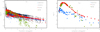 |
Fig. 1 Left panel: Fe I excitation rates (in s−1), log C, for electron impact (triangles) compared with rates of H I collisions from calculations of YBK18 (filled circles) and B18 (rhombi) and compared with the scaled (SH = 0.5) Drawinian rates (open circles). Right panel: rates, log C, of the processes Fe I + e−→ Fe II + 2e− and Fe I + H I → Fe II + H− using similarsymbols. The calculations were made with T = 5830 K, log Ne (cm−3) = 13, and log NH(cm−3) = 16.9. |
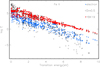 |
Fig. 2 Fe II excitation rates (in s−1), log C, for electron impact (triangles) compared with rates for H I collisions from calculations of YBK19 (filled circles) and compared with the scaled (SH = 0.5) Drawinian rates (open circles). The calculations were made with T = 5830 K, log Ne (cm−3) = 13, and log NH(cm−3) = 16.9. |
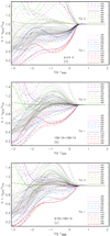 |
Fig. 3 Departure coefficients, b, for levels of Fe I and Fe II as a function of log τ5000 in model atmosphere 4600/1.40/ − 2.60 from calculations using different treatment of H I collisions: pure electronic collisions (top panel); YBK18 + YBK19 (middle panel); B18 + YBK19 (bottom panel). Every fifth of the first 60 levels (Eexc ≤ 5.73 eV) of Fe I is shown. They are quoted in the bottom right part of each panel. All levels of Fe I above Eexc = 7 eV areplotted by black dotted curves. For Fe II, we show every fifth of the first 60 levels (Eexc ≤ 8.16 eV). They are quoted in the top right part of each panel. The letters z, y, x, … are used to denote the odd parity terms, and a, b, c, … for the even parity terms. |
2.2 Statistical equilibrium of FeI–FeII
We chose the VMP model atmosphere, 4600/1.40/ − 2.60, to investigate the influence of inelastic collisions with H I and their different treatment on the SE of Fe I–Fe II. The calculations were performed for three different line-formation scenarios based on pure electronic collisions (a), including H I collisions for Fe I with the rate coefficients from YBK18 (b) and B18 (c). In both (b) and (c) cases, Fe II + H I collisions were accounted for using the data from YBK19. Figure 3 displays the departure coefficients, b = n_NLTE/n_LTE, for selected levels of Fe I and Fe II. Here, nNLTE and nLTE are the statistical equilibrium and thermal (Saha-Boltzmann) number densities, respectively.
As shown in the earlier NLTE studies (see Mashonkina et al. 2011, and references therein), the main NLTE mechanism for Fe I in the stellar parameter range, with which we are concerned here, is the ultra-violet (UV) over-ionisation caused by superthermal radiation of a non-local origin below the thresholds of the low excitation levels. It can be seen in Fig. 3 that the Fe I levels below  (Eexc ≃ 4.5 eV) are underpopulated at logτ5000 < 0.4, independent of the treatment of collisional rates. In the case of pure electronic collisions, even the highest levels of Fe I are strongly decoupled from the ground state of Fe II. As expected, the departures from LTE were smaller when collisions with H I were included. For example, at log τ5000 = −0.52, the departure coefficients of
  and
and  , which are the lower levels of the transitions, where the Fe I 5216 and 5586 Å lines arise, amounted to b = 0.36 and 0.40 in the case of pure electronic collisions, while they increased in the (b) and (c) scenarios: b(
 ) = 0.66 and 0.60 and b(
 ) = 0.71 and 0.69, respectively.
All the levels of Fe II below  (Eexc = 4.73 eV) have a common parity, and, independent of the treatment of collisional rates, they are closely coupled to the Fe II ground state throughout the atmosphere, except in the outermost layers. The odd-parity levels with Eexc ≥ 4.8 eV are affected by the pumped UV transitions from the ground, and low-excitation levels of Fe II. In the case of pure electronic collisions, this results in large overpopulation of all the levels above Eexc = 4.8 eV. Including collisions with H I substantially reduces the departures from LTE, in particular, for the levels below
  (Eexc = 6.7 eV).
3 Iron abundances and Fe I/Fe II ionisation equilibrium of reference stars
In this section, we test the updated model atom with the Fe I /Fe II ionisation equilibrium of the VMP stars with well-determined atmosphericparameters. We selected three Galactic halo stars, namely, HD 84937, HD 122563, and HD 140283, and a sample of 38 VMP stars in the dwarf spheroidal galaxies (dSphs) from Mashonkina et al. (2017, 35 stars) and Pakhomov et al. (2019, 3 stars).
3.1 Atmospheric parameters
Our analysis is based on photometric effective temperatures and distance based surface gravities. For a VMP giant HD 122563, coupling its angular diameter with photometry yields effective temperatures, which are fairly consistent in Creevey et al. (2012): Teff = 4598 ± 41 K and Karovicova et al. (2018): Teff = 4636 ± 37 K. Using a Gaia based distance of d = 288 pc from Bailer-Jones et al. (2018), and assuming the star’s mass M = 0.8 M⊙, we calculate log gd = 1.42 ± 0.02. This value agrees with log g = 1.39 ± 0.01, based on the detections of sun-like oscillations (Creevey et al. 2019). We adopted Teff = 4600 K and log g = 1.40 in our calculations. Based on our analysis of HD 122563 in Paper I, we used the model atmosphere with [Fe/H] = − 2.6. Both in NLTE and LTE, the slope of the logεFeI – log Wobs∕λ plot is largely removed with a microturbulent velocity of ξt = 1.6 km s−1. An accuracy of the ξt determination is estimated as0.2 km s−1. We note that our ξt value is consistent with the microturbulent velocity derived by Bergemann et al. (2012) and agrees within the error bars with ξt obtained by Amarsi et al. (2016) in their 1D-NLTE analysis. Hereafter, log εFeII and log εFeI are the Fe II and the Fe I based abundances, respectively. We used the scale where log εH = 12.
For HD 84937 and HD 140283, we took their Teff and log g from a careful analysis of Sitnova et al. (2015, hereafter, Paper II). For HD 140283, the adopted atmospheric parameters are supported by recent measurements: Karovicova et al. (2018) determine Teff = 5787 ± 48 K and a use of the Gaia DR2 parallax (Gaia Collaboration 2018) yields log g = 3.66 ± 0.03. In this study, we revise stellar metallicities, [Fe/H], using the Fe II lines in the visible spectral range and the solar abundance log ε⊙,FeII = 7.54 (Paper II), which is based on gf-values of Raassen & Uylings (1998). The microturbulent velocities were revised from a requirement that Fe I lines of different strength yield consistent absolute abundances. An accuracy of the ξt determination is estimated as 0.2 km s−1. For HD 84937, our ξt value agrees well with that obtained by Amarsi et al. (2016) in their 1D-NLTE analysis, while it is larger than that of Bergemann et al. (2012), by 0.3 km s−1. In contrast, our ξt value for HD 140283 is consistent with that of Bergemann et al. (2012).
For the dSph stars, we adopted their Teff, log g, [Fe/H], and ξt, as determined by Mashonkina et al. (2017) and Pakhomov et al. (2019). We did not revise microturbulent velocities, because applying new collisional data has minimal effect on the slopes of the logεFeI – log Wobs∕λ trends compared with the corresponding values in our previous studies.
Atmospheric parameters and iron abundances, log εFe, of the investigated stars.
LTE and NLTE abundances, log ε, from individual lines of Fe I and Fe II in HD 84937, HD 140283, and HD 122563.
3.2 Methods of abundance determinations
For the halo benchmark stars, both LTE and NLTE abundances were determined from line profile fitting. The synthetic spectra were computed with the SYNTHV_NLTE code (Tsymbal et al. 2019), which implements the pre-computed departure coefficients from the DETAIL code. The best fit to the observed spectrum was obtained automatically using the IDL BINMAG code by O. Kochukhov4. The line listand atomic data for the synthetic spectra calculations were taken from the VALD database (Ryabchikova et al. 2015). For the dSph stars, the NLTE abundances from individual lines were calculated by applying the NLTE abundance corrections computed in this study to the LTE abundances derived by Mashonkina et al. (2017) and Pakhomov et al. (2019).
3.3 Galactic halo benchmark stars
The atmospheric parameters and the average abundances for the two ionisation stages are presented in Table 1. Abundancesfrom individual lines are given in Table 2.
3.3.1 HD 122563
We used 32 lines of Fe I and 15 lines of Fe II in a high-quality spectrum from the ESO UVESPOP survey (Bagnulo et al. 2003). For Fe I, the line atomic data were taken from Paper I (their Table 5). The exceptions are Fe I 5242, 5662, and 5638 Å, for which we adopted the most recent gf-values from Belmonte et al. (2017), Den Hartog et al. (2014), and Ruffoni et al. (2014), respectively. We note that, for each of these three lines, their gf-values were upward revised, by 0.09–0.15 dex, and this led to larger line-to-line scatter in the Wobs < 12 mÅ equivalent width range (Fig. 4) compared with using the older data. For Fe II, we applied gf-values from Raassen & Uylings (1998). The exceptions are Fe II 4923 and 5018 Å, for which gf-values were obtained by averaging the data from the four sources with both lines available, namely, Bridges (1973), Moity (1983), Raassen & Uylings (1998, hereafter, RU98), and Meléndez & Barbuy (2009, hereafter, MB09).
In contrast to Paper I, we determine here absolute, but not differential abundances. They are derived in five different line-formation scenarios, namely: LTE, NLTE with pure electronic collisions, NLTE with including H I collisions and using the rate coefficients from YBK19 for Fe II and YBK18 or B18 for Fe I, and NLTE based on the Drawinian rates. Abundances from individual lines are shown in Fig. 4 for the first four cases. We comment on the results obtained in different line-formation scenarios.
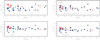 |
Fig. 4 LTE (top left panel) and NLTE (other three panels) abundances from lines of Fe I (circles) and Fe II (triangles) in HD 122563 as a function of observed equivalent width Wobs. Top right panel: NLTE calculations with pure electronic collisions. Bottom row, left and right panels: YBK18+YBK19 and B18+YBK19 scenarios, respectively. In each panel, the dotted line indicates the mean abundance derived from the Fe I lines. |
LTE
An abundance difference of − 0.25 dex is found between Fe I and Fe II.
Pure electronic collisions
The NLTE effects for lines of both Fe I and Fe II are substantially larger compared with those in the other NLTE scenarios (Fig. 5, only Fe I). For lines of Fe I, the NLTE abundance corrections, ΔNLTE = logεNLTE − logεLTE, are positive, and the obtained mean abundance, log εFeI = 5.11 ± 0.14, is 0.38 dex higher than the LTE value. Here, the sample standard deviation,  , determines the dispersion in the single line measurements around the mean for a given ionisation stage, and Nl is the number of measured lines. As discussed in Sect. 2.2, the Fe II levels above Eexc = 4.8 eV have large overpopulations in the case of pure electronic collisions. This results in positive NLTE corrections of ΔNLTE = 0.09–0.47 dex for lines of Fe II. The exceptions are Fe II 4923 and 5018 Å, for which ΔNLTE is slightly negative, of − 0.01 and − 0.03 dex, respectively. The mean NLTE abundance, logεFeII = 5.16 ± 0.21, is 0.18 dex higher than the LTE one, and we note large line-to-line scatter, resulting in σ, which is more than twice as big as in LTE.
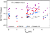 |
Fig. 5 NLTE abundance corrections for lines of Fe I in 4600/1.40/ − 2.60 model from calculations that use pure electronic collisions (squares) and include collisions with H I according to YBK18 (filled circles) and B18 (triangles). For comparison, the NLTE corrections were computed with the scaled Drawinian rates (SH = 0.5, open circles). |
Electronic + hydrogenic collisions
Independent of using either YBK18 or B18 data for Fe I + H I collisions, abundances from the two ionisation stages of iron are found to agree within the error bars. Although the NLTE abundance corrections for individual lines of Fe I can differ in these two scenarios, by up to 0.1 dex (Fig. 5). The exceptions are the Fe I 4427, 4920, and 5324 Å lines, for which the difference in ΔNLTE between B18 and YBK18 amounts to 0.17, 0.13, and 0.15 dex, respectively.
Including collisions with H I substantially reduces the NLTE effects for lines of Fe II, and ΔNLTEs are only slightlypositive (0.00–0.03 dex). The exceptions are the strongest Fe II 4923 and 5018 Å lines. Their cores form in the atmospheric layers, where the departure coefficient of the upper level drops below that of the lower level, resulting in dropping the line source function relatively to the Planck function and strengthened lines, such that ΔNLTE = −0.08 and − 0.09 dex, respectively.
In Paper I, we applied a line-by-line differential NLTE and LTE approach, in the sense that stellar line abundances were compared with individual abundances of their solar counterparts. Here, we find that, similarly to the non-differential analysis, the differential abundances from the two ionisation stages: [Fe/H]I = − 2.58 ± 0.11 (YBK18) and − 2.62 ± 0.11 (B18) and [Fe/H]II = − 2.55 ± 0.08 agree within the error bars.
 |
Fig. 6 NLTE abundances of HD 84937 (left panel) and HD 140283 (right panel) from lines of Fe I (circles) and Fe II (triangles) in the YBK18+YBK19 scenario as a function of observed equivalent width Wobs. The filled and open symbols correspond to the visible and UV lines, respectively. In each panel, the dotted line indicates the mean abundance derived from the Fe I visible lines. |
3.3.2 HD 84937 and HD 140283
For the visible spectral range, we used spectra from the ESO UVESPOP survey (Bagnulo et al. 2003). The line list is taken from Paper II, and it includes 12 lines of Fe I, and 7 lines of Fe II in HD 84937 and 20 and 14 lines in HD 140283. For lines of Fe I, we adopted the same gf-values, as in Paper II. The exceptions are Fe I 5242, 5379, and 5662 Å, for which the data were taken from Belmonte et al. (2017) and Den Hartog et al. (2014). As for HD 122563,we used gf-values of RU98 for lines of Fe II, with the exceptions for Fe II 4923 and 5018 Å.
This study extends analysis to the UV spectral range by using high-quality HST/STIS spectra in the 1875–3158 Å range, with a quality factor (QF) per resel of 52 and 90 for HD 84937 and HD 140283, respectively. Observations are provided by Thomas Ayres within the ASTRAL project5.
From a vast number of the Fe I lines in the UV spectrum of HD 140283, we selected those that are not blended, and have gf-values in O’Brian et al. (1991). The average LTE abundance from these lines is referred below as log εUV1. Then we appended some unblended lines with gf-values from Kurucz (2009) and Fuhr et al. (1988), which provide the abundance consistent with log εUV1, within 0.15 dex. For Fe I 2487 and 2730 Å, laboratory gf-values are taken from Belmonte et al. (2017). We find that the statistical error of the LTE abundance from Fe I lines decreases from 0.36 to 0.14 dex,when moving from a total list of 91 lines to the selected 42 lines. For 70 unblended lines of Fe II, with gf-values mostly from RU98, we obtained σ ≃ 0.15 dex. For Fe II 2262 and 2268 Å, gf-values are taken from Kroll & Kock (1987) and for Fe II 2254 Å from Pauls et al. (1990). No further pre-selection was made. We used a common list of the UV lines for HD 84937 and HD 140283. It includes 42 lines of Fe I and 70 lines of Fe II in the 1968–2990 Å wavelength range (Table 2).
The NLTE calculations were performed for the YBK18+YBK19 and B18+YBK19 line formation scenarios. Figure 6 shows abundances from individual lines for YBK18+YBK19.
For both stars, the NLTE effects for lines of Fe II are minor, with ΔNLTE < 0.01 dex. In case of Fe I, ΔNLTE is at the level of 0.15–0.2 dex for the Eexc < 2 eV lines, reaches a maximal value of ~0.4 dex for the lines arising from the  (Eexc ≃ 3.2 eV) and
  (Eexc ≃ 3.4 eV) levels and drops at Eexc > 4 eV (Fig. 7 only for HD 84937). The difference in ΔNLTE between using the YBK18 and B18 data does not exceed 0.05 and 0.07 dex for every Fe I line in HD 84937 and HD 140283, respectively.
For each star, both in LTE and NLTE and for both Fe I and Fe II, we obtained consistent (within 0.08 dex) abundances from the visible and UV lines. LTE leads to lower abundance from Fe I compared with that from Fe II, by 0.08 to 0.16 dex for different spectral ranges and different stars. In NLTE, the abundance difference log εFeI − log εFeII is positive andranges between 0.06 and 0.13 dex in different cases.
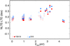 |
Fig. 7 NLTE abundance corrections for lines of Fe I in 6350/4.09/ − 2.15 model from calculations that include collisions with H I according to YBK18 (circles) and B18 (triangles). The filled and open symbols correspond to the visible and UV lines, respectively. |
3.4 Uncertainties in the derived iron abundances
For a given star, uncertainties in atmospheric parameters, applying different sources of the line atomic data, and different treatment of the NLTE line formation produce systematic shifts in the abundances derived from individual lines of a given chemical species. We evaluated their effects on the Fe I/Fe II ionisation equilibrium of the investigated stars, and the obtained results are summarised in Table 3. For comparison, the last string of Table 3 displays the statistical errors caused by line-to-line scatter,  . In test calculations, we varied Teff, log g, and ξt, by 50 K, 0.03 dex, and 0.2 km s−1, respectively, taking into account the aforementioned errors of their measurements. The string gf(MB09 – RU98) in Table 3 shows the changes in logεFeI − logεFeII, when replacing gf-values of RU98 with those of MB09 for the visible lines of Fe II.
Replacing photoionisation cross sections of Bautista et al. (2017, BLB2017) with the older ones of Bautista (1997, B1997) leads to slightly larger NLTE effects for Fe I lines in the 4600/1.4/ − 2.5 model atmosphere and nearly does not affect the NLTE results for the 6350/4.09/ − 2.15 and 5780/3.7/ − 2.4 models.
In the model atmosphere of HD 122563, a use of the B18 rate coefficients for Fe I + H I collisions leads to smaller NLTE effects for Fe I lines than those in the YBK18 case. In contrast, ΔNLTE(B18) > ΔNLTE(YBK18) for lines of Fe I in the atmospheres of HD 84937 and HD 140283. However, the abundance shifts do not exceed 0.03 dex.
For HD 122563, ignoring the Kaulakys (1991) collision rates produces minor shifts in the NLTE abundances derived from Fe I lines, of +0.02 and +0.03 dex, on average, in the B18 and YBK18 cases, respectively. Similarly small effects are found for HD 84937 and HD 140283. However, it is important to note that the abundance shifts have a different sign for the visible and the UV lines of Fe I. For example, for HD 140283, ignoring the Kaulakys (1991) collisions leads to higher abundances from the visible lines by 0.03 dex (YBK18) and < 0.01 dex (B18), yet to lower abundances from the UV lines, by 0.05 (YBK18) and 0.01 dex (B18). The abundance difference between the visible and the UV lines of Fe I decreases when the Kaulakys (1991) collisions are taken into account. We note that the similarly small effect of including the Kaulakys (1991) collisions on the abundance determinations from lines of Mn I is reported by Bergemann et al. (2019).
It can be seen that, for cool giants, achieving the Fe I/Fe II ionisation equilibrium depends firstly on an accuracy of Teff. The next important source of the abundance uncertainties is the gf-values. For example, applying gf-values of MB09 could remove the NLTE abundance difference logεFeI − logεFeII completely for HD 122563. We therefore call once more on atomic spectroscopists for further laboratory and theoretical works to improve gf-values of the Fe I and,in particular, Fe II lines used in abundance analysis. Taking into account the obtained statistical abundance errors, we conclude that none of the systematic effects can destroy the Fe I/Fe II ionisation equilibrium for the investigated halo benchmark stars.
Shifts in log εFeI − log εFeII caused by the uncertainties in atmospheric parameters, line atomic data, and NLTE treatment.
3.5 VMP giants in the dwarf spheroidal galaxies
Our sample of the dSph stars covers the − 4 ≤ [Fe/H] ≤−1.5 metallicity range that is useful for testing an updated model atom of Fe I-II, because the NLTE effects for Fe I lines depend on stellar metallicity. We used the same line list as in Mashonkina et al. (2017) and Pakhomov et al. (2019). The same atomic parameters are adopted for lines of Fe I, while, by analogy with analysis of the halo benchmark stars in Sect. 3.3, gf-values of RU98 are employed for the Fe II lines.
For each star, the NLTE calculations were performed with the YBK18+YBK19 collisional recipe. For lines of Fe II, the NLTE effects are minor at [Fe/H] > −3.7, such that ΔNLTE ≤ 0.02 dex, in absolute value. The exceptions are Fe II 4923 and 5018 Å, for which ΔNLTE is negative and can reach − 0.09 dex. At the lowest metallicity of our sample, [Fe/H] ~−4, the NLTE abundance corrections become positive for all the Fe II lines and reach +0.12 dex for 5197 Å and +0.06 dex for 5018 Å.
Figure 8 displays the NLTE abundance corrections for three Fe I lines with different Eexc. The departures from LTE for Fe I grow towards lower metallicity, for example, for Fe I 5216 Å, from ΔNLTE = 0.13 dex in the 4275/0.65/ − 2.08 model, to ΔNLTE = 0.39 dex in the 4800/1.56/ − 4.0 model. The NLTE corrections are larger, as a rule, for the higher than for the lower excitation line. For example, in the 4850/2.05/ − 2.96 model, ΔNLTE = 0.52, 0.25, and 0.20 dex for Fe I 5615 Å (Eexc = 3.33 eV), 6191 Å (Eexc = 2.43 eV), and 5216 Å (Eexc = 1.61 eV), respectively. Although the discrepancy between different lines decreases towards lower metallicity. Table 4 presents the average LTE and NLTE abundances of the dSph stars.
The abundance differences between Fe I and Fe II are displayed in Fig. 9. Under the LTE assumption, log εFeI is systematically lower than logεFeII, by − 0.27 ± 0.08 dex, on average. In the NLTE calculations, an abundance discrepancy is largely removed in the [Fe/H] > −3.5 regime, with the mean logεFeI – logεFeII = − 0.01 ± 0.10. At the lower metallicity, in five of six stars, abundances from Fe I lines are higher that those from Fe II, by up to 0.35 dex. As discussed by Mashonkina et al. (2017), this could be due to overestimated effective temperatures that were determined for these stars from photometric colours. From a careful analysis of a sample of the UMP stars, Sitnova et al. (2019) recommend using as many photometric and spectroscopic indicators of Teff and log g as possible, in order to improve the accuracy of derived atmospheric parameters. In this study, we did not aim to revise Teff s of our sample stars.
Analysis of the Fe I/Fe II ionisation equilibrium in the same dSph stars by Mashonkina et al. (2017) was different to the present one in two aspects: collisions with H I were treated with the Drawinian rates, and abundances from the Fe II lines were derived with gf-values of Raassen & Uylings (1998), which were corrected by + 0.11 dex, following the recommendation of Grevesse & Sauval (1999). In order to achieve consistent abundances from the two ionisation stages for the stars at [Fe/H] > −3.5, Mashonkina et al. (2017) applied a scaling factor of SH = 0.5 to the Drawinian rates. With the quantum mechanical rate coefficients from YBK18, we calculate larger NLTE abundance corrections for Fe I lines, by 0.1 dex, on average. Therefore, a use of the scaled (SH = 0.5) Drawinian rates, together with the corrected (by + 0.11 dex) gf-values of Raassen & Uylings (1998), provides, on average, the same abundance difference between Fe I and Fe II as that for accurate collisional data together with original gf-values of Raassen & Uylings (1998).
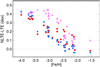 |
Fig. 8 NLTE abundance corrections for Fe I 5216 Å (Eexc = 1.61 eV, red circles), 6191 Å (Eexc = 2.43 eV, blue squares), and 5615 Å (Eexc = 3.33 eV, magenda triangles) in dSph stars from calculations with YBK18 data. |
Iron NLTE abundances, log ε, of the dSph stars from calculations with the YBK18+YBK19 recipe.
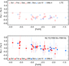 |
Fig. 9 LTE (top panel) and NLTE (YBK18+YBK19, bottom panel) abundance differences between Fe I and Fe II, log εFeI – log εFeII, in stars in Sculptor (red circles), Ursa Minor (red triangles), Fornax (red rhombi), Sextans (red squares), Boötes I (blue circles), UMa II (blue inverted triangles), and Leo IV (blue five-pointed star) dSphs. The error bars correspond to σFeI - FeII. |
4 Comparison with other studies
For the halo benchmark stars discussed in Sect. 3.3, the iron abundance analyses were performed by Amarsi et al. (2016, hereafter, ALA16) based on detailed 3D NLTE radiative transfer calculations using 3D hydrodynamic STAGGER model atmospheres. They treated Fe I + H I collisions with quantum-mechanical rate coefficients from Barklem (2016). We do not compare the results for HD 140283 here because of large discrepancy in Teff between this study (5780 K) and ALA16 (5591 K). For HD 84937, ALA16 adopted Teff = 6356 K, log g = 4.06, and [Fe/H] = − 2.0, which are close to ours. Our LTE abundances from lines of both Fe I and Fe II in the visible spectral range agree with the corresponding 1D LTE abundances of ALA16, within 0.04 dex. We obtained slightly stronger NLTE effects for Fe I lines, with the mean NLTE – LTE abundance difference of +0.22(YBK18)/0.24 dex (B18), while the 1D NLTE analysis from ALA16 results in +0.17 dex.
In order to compare the results for HD 122563, we took the same atmospheric parameters, Teff = 4600 K, log g = 1.6, and [Fe/H] = − 2.5, as in ALA16. In LTE, we obtained higher abundances than those of ALA16, by 0.13 and 0.10 dex for Fe I and Fe II, respectively. The NLTE – LTE abundance differences amount to 0.15 (YBK18) and 0.13 dex (B18) for Fe I, while ALA16 reported 0.09 dex. The discrepancies in both LTE and NLTE abundances could be due to the use of different line lists.
Interestingly, the 3D NLTE analyses from ALA16 led to the higher abundances compared with the 1D NLTE ones, by a very similar amount for Fe I and Fe II in a given star: by 0.12 and 0.10 dex, respectively, in HD 84937 and by 0.08 and 0.07 dex in HD 122563. This leads us to think that the NLTE abundance discrepancy of 0.1 dex between Fe I and Fe II obtained in this study for the visible lines in HD 84937 and HD 140283 could not be removed when applying the 3D NLTE analysis.
For HD 84937, the Fe I/Fe II ionisation equilibrium based not only on visible, but also UV spectra was checked earlier by Sneden et al. (2016, hereafter, S16) and Roederer et al. (2018, hereafter, R18) under the LTE assumption. Both studies usedthe VLT/UVES spectrum in the visible range, but different STIS UV spectra, with a resolution of R = 25 000 and 114 000, respectively. Despite employing rather different atmospheric parameters, namely, Teff /log g = 6300 K/4.00 (S16) and 6418 K/4.16 (R18), these two papers reported close together abundances, and each of them obtained a perfect agreement between the two ionisation stages, Fe I and Fe II. From 446 lines of Fe I and 105 lines of Fe II, S16 derived log εFeI = 5.20 and logεFeII = 5.19. Using the solar abundances presented by S16 in their Table 1, we calculated identical values: [Fe/H]I = [Fe/H]II = −2.32. In their Table 8, R18 present [Fe/H]I = −2.26 from 164 lines with Eexc > 1.2 eV and [Fe/H]II = −2.23 from 27 lines.
Our list of the UV lines has 20 lines of Fe I and six lines of Fe II in common with S16, yet no common line with R18. By averaging our results from the visible and UV lines, we obtained the LTE abundance log εFeI = 5.23, in line with that of S16 and R18. Our logεFeII is higher than that of S16, by 0.11 dex, and agrees within 0.02 dex with that of R18. A discrepancy with S16 could be due to different line lists and different gf-values. When using the same gf-values, as in S16 for common lines, we obtained a difference of less than 0.01 dex in log εFeII between this study and S16.
5 Conclusions
In this study, the Fe I–Fe II model atom of Mashonkina et al. (2011) is updated by implementing photoionisation cross sections for the Fe I levels from Bautista et al. (2017), electron-impact excitation data from Bautista et al. (2017) for the Fe I transitions, and by including inelastic Fe I + H I and Fe II + H I collisions with rate coefficients from quantum-mechanical calculations of Barklem (2018, Fe I), Yakovleva et al. (2018a, Fe I), and Yakovleva et al. (2019, Fe II). We also implement the Kaulakys (1991) collisions, applying rate coefficients from Barklem (2017) calculations.
Using classical 1D model atmospheres, we inspect the effect of H I collisions and their different treatment on the derived abundances and the Fe I /Fe II ionisation equilibrium of the three Galactic halo benchmark stars and a sample of 38 VMP giants in the dwarf galaxies with well known distances. For each star, the average NLTE abundances from Fe I lines obtained using the data of Yakovleva et al. (2018a) and Barklem (2018) differ by no more than 0.03 dex. Although discrepancies in the NLTE abundance corrections for individual lines exist, in most cases, they do not exceed 0.1 dex. The exceptions are the Fe I 4427, 4920, and 5324 Å lines in HD 122563, for which the difference in ΔNLTE amounts to 0.17, 0.13, and 0.15 dex, respectively. Further theoretical works are needed to improve the theory of inelastic Fe I + H I collisions.
The obtained results can be summarized as follows.
- 1.
Collisions with H I serve as efficient thermalisation sources for Fe II, such that the NLTE abundance corrections for Fe II lines do not exceed 0.02 dex, in absolute value, at [Fe/H] ≳ − 3 and can reach +0.06 dex at [Fe/H] ~−4. Thus, in a broad metallicity range, except for the ultra-metal poor stars, lines of Fe II can be safely used under the LTE assumption as abundance indicators.
- 2.
For the VMP giants, the NLTE abundances from the two ionisation stages agree within the error bars, with log εFeI – log εFeII = − 0.07 (YBK18) and − 0.09 (B18) for HD 122563 and − 0.01 ± 0.10 for 32 stars in the dSphs at [Fe/H] > −3.5. For comparison, the corresponding LTE abundance differences amount to − 0.25 and − 0.27 ± 0.08 dex.
- 3.
Using the 1960–6460 Å spectra, we obtain an abundance discrepancy of 0.10 (YBK18)/0.13 (B18) and 0.09 (YBK18)/0.12 (B18) between Fe I and Fe II in a VMP turn-off star HD 84937 and a VMP subgiant HD 140283, respectively. For either Fe I or Fe II in each star, abundances from the visible and UV lines are found to be consistent within 0.08 dex.
Acknowledgements
We are grateful to Paul Barklem and Manuel Bautista for providing the rate coefficients for Fe I + H I collisions and photoionisation cross sections for Fe I publicly available. The authors thank the Russian Science Foundation (grant 17-13-01144) for a partial support of this study. We made use of the ESO UVESPOP and the ASTRAL spectral archives and the ADS6, SIMBAD7, and VALD databases.
References
- Amarsi, A. M., Lind, K., Asplund, M., Barklem, P. S., & Collet, R. 2016, MNRAS, 463, 1518 [NASA ADS] [CrossRef] [Google Scholar]
- Bagnulo, S., Jehin, E., Ledoux, C., et al. 2003, The Messenger, 114, 10 [Google Scholar]
- Bailer-Jones, C. A. L., Rybizki, J., Fouesneau, M., Mantelet, G., & Andrae, R. 2018, AJ, 156, 58 [NASA ADS] [CrossRef] [Google Scholar]
- Barklem, P. S. 2016, Phys. Rev. A, 93, 042705 [NASA ADS] [CrossRef] [Google Scholar]
- Barklem, P. S. 2017, Astrophysics Source Code Library [record ascl:1701.005] [Google Scholar]
- Barklem, P. S. 2018, A&A, 612, A90 [NASA ADS] [CrossRef] [EDP Sciences] [Google Scholar]
- Bautista, M. A. 1997, A&AS, 122, 167 [NASA ADS] [CrossRef] [EDP Sciences] [Google Scholar]
- Bautista, M. A., & Pradhan, A. K. 1996, A&AS, 115, 551 [NASA ADS] [Google Scholar]
- Bautista, M. A., & Pradhan, A. K. 1998, ApJ, 492, 650 [NASA ADS] [CrossRef] [Google Scholar]
- Bautista, M. A., Lind, K., & Bergemann, M. 2017, A&A, 606, A127 [NASA ADS] [CrossRef] [EDP Sciences] [Google Scholar]
- Belmonte, M. T., Pickering, J. C., Ruffoni, M. P., et al. 2017, ApJ, 848, 125 [NASA ADS] [CrossRef] [Google Scholar]
- Bensby, T., Feltzing, S., & Oey, M. S. 2014, A&A, 562, A71 [NASA ADS] [CrossRef] [EDP Sciences] [Google Scholar]
- Bergemann, M., Lind, K., Collet, R., Magic, Z., & Asplund, M. 2012, MNRAS, 427, 27 [NASA ADS] [CrossRef] [Google Scholar]
- Bergemann, M., Ruchti, G. R., Serenelli, A., et al. 2014, A&A, 565, A89 [NASA ADS] [CrossRef] [EDP Sciences] [Google Scholar]
- Bergemann, M., Gallagher, A. J., Eitner, P., et al. 2019, A&A, in press, https://doi.org/10.1051/0004-6361/201935811 [Google Scholar]
- Boyarchuk, A. A., Lyubimkov, L. S., & Sakhibullin, N. A. 1985, Astrophysics, 22, 203 [NASA ADS] [CrossRef] [Google Scholar]
- Bridges, J. M. 1973, in Phenomena in Ionized Gases, Eleventh International Conference, ed. I. Štoll, 418 [Google Scholar]
- Butler, K., & Giddings, J. 1985, Newsletter on the analysis of astronomical spectra, No. 9, University of London [Google Scholar]
- Creevey, O. L., Thévenin, F., Boyajian, T. S., et al. 2012, A&A, 545, A17 [NASA ADS] [CrossRef] [EDP Sciences] [Google Scholar]
- Creevey, O., Grundahl, F., Thévenin, F., et al. 2019, A&A, 625, A33 [NASA ADS] [CrossRef] [EDP Sciences] [Google Scholar]
- Den Hartog, E. A., Ruffoni, M. P., Lawler, J. E., et al. 2014, ApJS, 215, 23 [NASA ADS] [CrossRef] [Google Scholar]
- Drawin, H.-W. 1968, Z. Phys., 211, 404 [NASA ADS] [CrossRef] [EDP Sciences] [Google Scholar]
- Drawin, H. W. 1969, Z. Phys., 225, 483 [NASA ADS] [CrossRef] [EDP Sciences] [Google Scholar]
- Fuhr, J. R., Martin, G. A., & Wiese, W. L. 1988, J. Phys. Chem. Ref. Data, 17, 504 [Google Scholar]
- Gaia Collaboration (Brown, A. G. A., et al.) 2018, A&A, 616, A1 [NASA ADS] [CrossRef] [EDP Sciences] [Google Scholar]
- Gehren, T., Butler, K., Mashonkina, L., Reetz, J., & Shi, J. 2001, A&A, 366, 981 [NASA ADS] [CrossRef] [EDP Sciences] [Google Scholar]
- Gigas, D. 1986, A&A, 165, 170 [Google Scholar]
- Gratton, R. G., Carretta, E., Eriksson, K., & Gustafsson, B. 1999, A&A, 350, 955 [NASA ADS] [Google Scholar]
- Grevesse, N., & Sauval, A. J. 1999, A&A, 347, 348 [NASA ADS] [Google Scholar]
- Grupp, F., Kurucz, R. L., & Tan, K. 2009, A&A, 503, 177 [NASA ADS] [CrossRef] [EDP Sciences] [Google Scholar]
- Gustafsson, B., Edvardsson, B., Eriksson, K., et al. 2008, A&A, 486, 951 [NASA ADS] [CrossRef] [EDP Sciences] [Google Scholar]
- Karovicova, I., White, T. R., Nordlander, T., et al. 2018, MNRAS, 475, L81 [NASA ADS] [CrossRef] [Google Scholar]
- Kaulakys, B. 1991, J. Phys. B At. Mol. Phys., 24, L127 [Google Scholar]
- Korn, A. J., Shi, J., & Gehren, T. 2003, A&A, 407, 691 [NASA ADS] [CrossRef] [EDP Sciences] [Google Scholar]
- Kroll, S., & Kock, M. 1987, A&AS, 67, 225 [NASA ADS] [Google Scholar]
- Kurucz, R. L. 1992, Rev. Mex. Astron. Astrofis., 23, 181 [Google Scholar]
- Kurucz, R. L. 2009, Robert L. Kurucz on-line database of observed and predicted atomic transitions [Google Scholar]
- Lind, K., Bergemann, M., & Asplund, M. 2012, MNRAS, 427, 50 [NASA ADS] [CrossRef] [Google Scholar]
- Lind, K., Amarsi, A. M., Asplund, M., et al. 2017, MNRAS, 468, 4311 [NASA ADS] [CrossRef] [EDP Sciences] [Google Scholar]
- Mashonkina, L., Gehren, T., Shi, J.-R., Korn, A. J., & Grupp, F. 2011, A&A, 528, A87 [NASA ADS] [CrossRef] [EDP Sciences] [Google Scholar]
- Mashonkina, L., Jablonka, P., Pakhomov, Y., Sitnova, T., & North, P. 2017, A&A, 604, A129 [NASA ADS] [CrossRef] [EDP Sciences] [Google Scholar]
- Meléndez, J.,& Barbuy, B. 2009, A&A, 497, 611 [NASA ADS] [CrossRef] [EDP Sciences] [Google Scholar]
- Moity, J. 1983, A&AS, 52, 37 [NASA ADS] [Google Scholar]
- Nave, G., Johansson, S., Learner, R. C. M., Thorne, A. P., & Brault, J. W. 1994, ApJS, 94, 221 [NASA ADS] [CrossRef] [Google Scholar]
- O’Brian, T. R., Wickliffe, M. E., Lawler, J. E., Whaling, W., & Brault, J. W. 1991, J. Opt. Soc. Am. B Opt. Phys., 8, 1185 [NASA ADS] [CrossRef] [Google Scholar]
- Pakhomov, Y., Mashonkina, L., Sitnova, T., & Jablonka, P. 2019, Astron. Lett., 45, 303 [Google Scholar]
- Pauls, U., Grevesse, N., & Huber, M. C. E. 1990, A&A, 231, 536 [NASA ADS] [Google Scholar]
- Raassen, A. J. J., & Uylings, P. H. M. 1998, A&A, 340, 300 [Google Scholar]
- Roederer, I. U., Sneden, C., Lawler, J. E., et al. 2018, ApJ, 860, 125 [NASA ADS] [CrossRef] [Google Scholar]
- Ruchti, G. R., Bergemann, M., Serenelli, A., Casagrande, L., & Lind, K. 2013, MNRAS, 429, 126 [NASA ADS] [CrossRef] [Google Scholar]
- Ruffoni, M. P., Den Hartog, E. A., Lawler, J. E., et al. 2014, MNRAS, 441, 3127 [NASA ADS] [CrossRef] [Google Scholar]
- Ryabchikova, T., Piskunov, N., Kurucz, R. L., et al. 2015, Phys. Scr., 90, 054005 [NASA ADS] [CrossRef] [Google Scholar]
- Seaton, M. J. 1962, in Atomic and Molecular Processes, ed. D. R. Bates (Amsterdam: Elsevier), 375 [Google Scholar]
- Shchukina, N., & Trujillo Bueno, J. 2001, ApJ, 550, 970 [NASA ADS] [CrossRef] [Google Scholar]
- Sitnova, T., Zhao, G., Mashonkina, L., et al. 2015, ApJ, 808, 148 [Google Scholar]
- Sitnova, T. M., Mashonkina, L. I., Ezzeddine, R., & Frebel, A. 2019, MNRAS, 485, 3527 [NASA ADS] [CrossRef] [Google Scholar]
- Sneden, C., Cowan, J. J., Kobayashi, C., et al. 2016, ApJ, 817, 53 [NASA ADS] [CrossRef] [Google Scholar]
- Steenbock, W., & Holweger, H. 1984, A&A, 130, 319 [NASA ADS] [Google Scholar]
- Tanaka, K. 1971, PASJ, 23, 217 [NASA ADS] [Google Scholar]
- Tsymbal, V., Ryabchikova, T., & Sitnova, T. 2019, ASP Conf. Ser., 518, 247 [NASA ADS] [Google Scholar]
- Yakovleva, S. A., Belyaev, A. K., & Kraemer, W. P. 2018a, Chem. Phys., 515, 369 [CrossRef] [Google Scholar]
- Yakovleva, S. A., Barklem, P. S., & Belyaev, A. K. 2018b, MNRAS, 473, 3810 [NASA ADS] [CrossRef] [Google Scholar]
- Yakovleva, S. A., Belyaev, A. K., & Kraemer, W. P. 2019, MNRAS, 483, 5105 [NASA ADS] [CrossRef] [Google Scholar]
- Zhang, H. L., & Pradhan, A. K. 1995, A&A, 293, 953 [NASA ADS] [Google Scholar]
In the classical notation, where [X/H] =  .
.
All Tables
LTE and NLTE abundances, log ε, from individual lines of Fe I and Fe II in HD 84937, HD 140283, and HD 122563.
Shifts in log εFeI − log εFeII caused by the uncertainties in atmospheric parameters, line atomic data, and NLTE treatment.
Iron NLTE abundances, log ε, of the dSph stars from calculations with the YBK18+YBK19 recipe.
All Figures
|
Fig. 1 Left panel: Fe I excitation rates (in s−1), log C, for electron impact (triangles) compared with rates of H I collisions from calculations of YBK18 (filled circles) and B18 (rhombi) and compared with the scaled (SH = 0.5) Drawinian rates (open circles). Right panel: rates, log C, of the processes Fe I + e−→ Fe II + 2e− and Fe I + H I → Fe II + H− using similarsymbols. The calculations were made with T = 5830 K, log Ne (cm−3) = 13, and log NH(cm−3) = 16.9. |
| In the text | |
|
Fig. 2 Fe II excitation rates (in s−1), log C, for electron impact (triangles) compared with rates for H I collisions from calculations of YBK19 (filled circles) and compared with the scaled (SH = 0.5) Drawinian rates (open circles). The calculations were made with T = 5830 K, log Ne (cm−3) = 13, and log NH(cm−3) = 16.9. |
| In the text | |
|
Fig. 3 Departure coefficients, b, for levels of Fe I and Fe II as a function of log τ5000 in model atmosphere 4600/1.40/ − 2.60 from calculations using different treatment of H I collisions: pure electronic collisions (top panel); YBK18 + YBK19 (middle panel); B18 + YBK19 (bottom panel). Every fifth of the first 60 levels (Eexc ≤ 5.73 eV) of Fe I is shown. They are quoted in the bottom right part of each panel. All levels of Fe I above Eexc = 7 eV areplotted by black dotted curves. For Fe II, we show every fifth of the first 60 levels (Eexc ≤ 8.16 eV). They are quoted in the top right part of each panel. The letters z, y, x, … are used to denote the odd parity terms, and a, b, c, … for the even parity terms. |
| In the text | |
|
Fig. 4 LTE (top left panel) and NLTE (other three panels) abundances from lines of Fe I (circles) and Fe II (triangles) in HD 122563 as a function of observed equivalent width Wobs. Top right panel: NLTE calculations with pure electronic collisions. Bottom row, left and right panels: YBK18+YBK19 and B18+YBK19 scenarios, respectively. In each panel, the dotted line indicates the mean abundance derived from the Fe I lines. |
| In the text | |
|
Fig. 5 NLTE abundance corrections for lines of Fe I in 4600/1.40/ − 2.60 model from calculations that use pure electronic collisions (squares) and include collisions with H I according to YBK18 (filled circles) and B18 (triangles). For comparison, the NLTE corrections were computed with the scaled Drawinian rates (SH = 0.5, open circles). |
| In the text | |
|
Fig. 6 NLTE abundances of HD 84937 (left panel) and HD 140283 (right panel) from lines of Fe I (circles) and Fe II (triangles) in the YBK18+YBK19 scenario as a function of observed equivalent width Wobs. The filled and open symbols correspond to the visible and UV lines, respectively. In each panel, the dotted line indicates the mean abundance derived from the Fe I visible lines. |
| In the text | |
|
Fig. 7 NLTE abundance corrections for lines of Fe I in 6350/4.09/ − 2.15 model from calculations that include collisions with H I according to YBK18 (circles) and B18 (triangles). The filled and open symbols correspond to the visible and UV lines, respectively. |
| In the text | |
|
Fig. 8 NLTE abundance corrections for Fe I 5216 Å (Eexc = 1.61 eV, red circles), 6191 Å (Eexc = 2.43 eV, blue squares), and 5615 Å (Eexc = 3.33 eV, magenda triangles) in dSph stars from calculations with YBK18 data. |
| In the text | |
|
Fig. 9 LTE (top panel) and NLTE (YBK18+YBK19, bottom panel) abundance differences between Fe I and Fe II, log εFeI – log εFeII, in stars in Sculptor (red circles), Ursa Minor (red triangles), Fornax (red rhombi), Sextans (red squares), Boötes I (blue circles), UMa II (blue inverted triangles), and Leo IV (blue five-pointed star) dSphs. The error bars correspond to σFeI - FeII. |
| In the text | |
Current usage metrics show cumulative count of Article Views (full-text article views including HTML views, PDF and ePub downloads, according to the available data) and Abstracts Views on Vision4Press platform.
Data correspond to usage on the plateform after 2015. The current usage metrics is available 48-96 hours after online publication and is updated daily on week days.
Initial download of the metrics may take a while.