| Issue |
A&A
Volume 631, November 2019
|
|
|---|---|---|
| Article Number | A178 | |
| Number of page(s) | 8 | |
| Section | The Sun | |
| DOI | https://doi.org/10.1051/0004-6361/201935121 | |
| Published online | 19 November 2019 | |
Readdressing the UV solar variability with SATIRE-S: non-LTE effects
1
Blackett Laboratory, Astrophysics Group, Imperial College, London SW7 2AZ, UK
e-mail: This email address is being protected from spambots. You need JavaScript enabled to view it.
2
Max-Planck Institute for Solar System Research, 37077 Göttingen, Germany
3
School of Space Research, Kyung Hee University, 446-701 Yongin, Gyeonggi-Do, South Korea
Received:
24
January
2019
Accepted:
27
September
2019
Abstract
Context. Solar spectral irradiance (SSI) variability is one of the key inputs to models of the Earth’s climate. Understanding solar irradiance fluctuations also helps to place the Sun among other stars in terms of their brightness variability patterns and to set detectability limits for terrestrial exoplanets.
Aims. One of the most successful and widely used models of solar irradiance variability is Spectral And Total Irradiance REconstruction model (SATIRE-S). It uses spectra of the magnetic features and surrounding quiet Sun that are computed with the ATLAS9 spectral synthesis code under the assumption of local thermodynamic equilibrium (LTE). SATIRE-S has been at the forefront of solar variability modelling, but due to the limitations of the LTE approximation its output SSI has to be empirically corrected below 300 nm, which reduces the physical consistency of its results. This shortcoming is addressed in the present paper.
Methods. We replaced the ATLAS9 spectra of all atmospheric components in SATIRE-S with spectra that were calculated using the Non-LTE Spectral SYnthesis (NESSY) code. To compute the spectrum of the quiet Sun and faculae, we used the temperature and density stratification models of the FAL set.
Results. We computed non-LTE contrasts of spots and faculae and combined them with the corresponding fractional disc coverages, or filling factors, to calculate the total and spectral irradiance variability during solar cycle 24. The filling factors have been derived from solar full-disc magnetograms and continuum images recorded by the Helioseismic and Magnetic Imager on Solar Dynamics Observatory (SDO/HMI).
Conclusions. The non-LTE contrasts yield total and spectral solar irradiance variations that are in good agreement with empirically corrected LTE irradiance calculations. This shows that the empirical correction applied to the SATIRE-S total and spectral solar irradiance is consistent with results from non-LTE computations.
Key words: Sun: activity / Sun: atmosphere / sunspots / Sun: faculae / plages / Sun: UV radiation / radiative transfer
© ESO 2019
1. Introduction
The variability of the solar spectral irradiance is one of the drivers of the chemistry and dynamics in the Earth’s middle atmosphere (Brasseur & Solomon 2005; Haigh 2007), and it may affect the terrestrial climate (Haigh 1994; Soukharev & Hood 2006; Austin et al. 2008; Haigh et al. 2010; Solanki et al. 2013; Mitchell et al. 2015). To understand the nature and the degree of this influence, and thus disentangle it from the anthropogenic causes of climate change, chemistry-climate models have been developed in which solar irradiance is a key input component.
Studies of solar irradiance variability also help to understand the variability of other stars, while a comparison of the solar variability pattern to that of other lower main sequence stars helps to understand the place of the Sun among them (e.g. Basri et al. 2013; Shapiro et al. 2013, 2014). Furthermore, stellar variability is a limiting factor for the detection of terrestrial exoplanets (Saar & Donahue 1997; Aigrain et al. 2004; Desort et al. 2007; Pont et al. 2008; Lagrange et al. 2010; Gilliland et al. 2011), which calls for realistic models of stellar brightness variations (Boisse et al. 2012; Korhonen et al. 2015). It is important to note that the extension of the exoplanetary search mission Kepler (Batalha 2014) was granted due to higher than expected stellar variability (Gilliland et al. 2015).
Gaining an understanding of the solar-terrestrial and solar-stellar connections requires sufficiently long, uninterrupted, and reliable records of solar spectral irradiance. The available measurements only fulfil these requirements in part. The total solar irradiance (TSI), which is the spectrally integrated radiant flux received per unit surface area at 1 AU from the Sun, has been monitored almost continuously by a series of missions since 1978 (see, e.g. Kopp 2016). The measurements of spectral solar irradiance (SSI), that is radiant flux per unit surface area and unit wavelength at 1 AU from the Sun, are significantly less homogeneous. The records have numerous gaps both in time and wavelength, and they exhibit significant instrumental trends (see Yeo et al. 2015). Thus models of the solar irradiance variability were developed to allow reconstructions with a more complete coverage, both in time and wavelength (see, e.g. Solanki et al. 2013, for a review).
The first generation of solar irradiance models relies on empirical correlations between the measured irradiance and proxies of solar magnetic activity. The more advanced semi-empirical models use 1D representations of temperature and density stratifications of active and quiet components of the Sun (solar model atmospheres) and radiative transfer codes to calculate their spectra. This second generation of models, having at their core a more robust physical approach, provide insights into understanding the physics behind the empirical correlations. In particular, Krivova et al. (2003), Ball et al. (2012), and Yeo et al. (2014) show that over 96% of TSI variations during cycles 23 and 24 on timescales of a day and longer can be explained by the evolution of the magnetic field at the solar surface alone.
Among the semi-empirical models, the Spectral And Total Irradiance REconstruction model (SATIRE-S, Fligge et al. 2000; Krivova et al. 2011) is one of the most successful. The index “S” stands for the version of the model based on satellite data, that is full-disc continuum images and magnetograms. SATIRE-S employs the local thermodynamic equilibrium (LTE) radiative transfer code ATLAS9 (Kurucz 1992; Castelli & Kurucz 1994) to calculate spectra that emerge from the active (i.e. strongly magnetised) and quiet regions of the Sun. Because of this LTE limitation, the SSI calculated with SATIRE-S is subject to empirical correction below 300 nm (Krivova et al. 2006; Yeo et al. 2014). Thus, in the range between 180 nm and 300 nm, the absolute level of the irradiance is shifted to match that of the WHI spectrum (Woods et al. 2009). Below 180 nm, in addition to the shift in the absolute level, the magnitude of the rotational and solar-cycle variability is scaled to agree with the measurements by the SOLar-STellar Irradiance Comparison Experiment (SOLSTICE, McClintock et al. 2005) on board SOlar Radiation and Climate Experiment (SORCE, Rottman 2005). Although the results of this scaling provide rather accurate TSI and satisfactory SSI reconstructions, such an ad hoc step is unsatisfactory. In addition, there are strong spectral lines in this wavelength range whose variability is poorly reproduced in LTE, irrespective of the scaling.
Unfortunately, this weakness of SATIRE-S is particularly pronounced in the most controversial spectral range from 200 nm to 400 nm. The irradiance variability in this range is important for climate studies (Ermolli et al. 2013; Ball et al. 2014a,b, 2016; Maycock et al. 2015, 2016). The fact that the magnitude of the variability in this range differs between the different models and the measurements is vexing (Krivova et al. 2006; Harder et al. 2009; Unruh et al. 2012; Yeo et al. 2015, 2017a). Empirical models tend to return variability amplitudes that are almost a factor of two lower than semi-empirical models suggest (Thuillier et al. 2014; Yeo et al. 2014, 2015, 2017a; Egorova et al. 2018), while the insufficient stability of most instruments (Yeo et al. 2015) compared to the solar cycle variability above 250–400 nm does not allow one to decide between these different amplitudes.
In this paper we used the Non-LTE Spectral SYnthesis (NESSY) code (Tagirov et al. 2017) to compute the emergent spectra of the various atmospheric components used in SATIRE-S and to model SSI variability over cycle 24 without the need for any empirical corrections. We emphasise that the aim of this paper is not to update the SATIRE-S model, but rather to compare LTE and non-LTE active region contrasts and to verify the model in the UV part of the solar spectrum. In Sect. 2 we give a description of SATIRE-S and the verification procedure, in Sect. 3 we discuss the results, and in Sect. 4 we summarise our results and provide conclusions and the outlook for the future.
2. Model description
The SATIRE-S model returns daily values of solar irradiance in the wavelength range from 115 nm to 160 000 nm. The model operates under the assumption that the solar irradiance variability on timescales longer than a day is driven by the magnetic active regions on the surface of the Sun and has two main components: the fractional coverages of the solar disc by these regions and their synthesised intensity spectra. The active regions included in the model are spots (consisting of umbra and penumbra components), which reduce solar irradiance as they pass across the solar disc, and faculae, which have the opposite effect (at wavelengths up to about 1500 nm). SSI, as a function of time t and wavelength λ, can be written as
 (1)
(1)
where j ∈ {f, p, u} and Iq, If, Ip, Iu are the intensities emerging from quiet Sun, faculae, penumbra and umbra respectively. The intensities are functions of wavelength and of the cosine of heliospheric angle μi. The solar disc has been subdivided into concentric rings (indexed with i) covering an equally large μ range. The integration over the solar disc is represented by the summation over the concentric rings. Furthermore, αji are the time-dependent fractional coverages (or filling factors) of the ith ring by the faculae, penumbrae and umbrae, Cj(λ, μi) is the brightness contrast of magnetic feature j, ΔΩi is the solid angle extended by the ith ring as seen from the Earth and Sq(λ) is the full disc quiet Sun radiative flux at wavelength λ.
In SATIRE-S, the surface coverages by faculae and sunspots are derived from the continuum intensity images and magnetograms taken by the National Solar Observatory, Kitt Peak, USA (NSO/KP), the Michelson Doppler Imager on-board Solar and Heliospheric Observatory (SOHO/MDI), and the Helioseismic and Magnetic Imager on-board Solar Dynamics Observatory (SDO/HMI; see Yeo et al. 2014, for more detail). Here we only consider the period from 2010 to 2017 covered by the superior space-borne SDO/HMI observations. We stress once more that our aim is to validate SATIRE’s variability in the UV range, rather than a full update of the model.
The filling factors are given by the ratio of the area (in pixels) covered by a particular type of feature (faculae, sunspot umbrae or penumbrae) to the total area of the ith ring. Both spots and faculae are seen in magnetograms, but only spots are seen in the intensity images as dark regions. Therefore, by combining these two types of images one can deduce whether a given pixel has facular signal. Faculae are composed of a multitude of magnetic elements, whose sizes are such that they do not always fill the area of an entire pixel. If a pixel is magnetic and does not belong to a spot, then a fraction of this pixel is attributed to faculae. This fraction is linearly proportional to the magnetic signal coming from the pixel up to a saturation value Bsat (Fligge et al. 2000), above which the pixel is assumed to be completely covered by faculae. Bsat is a free parameter in the model and its optimal value is determined by varying it until best agreement is reached between modelled and measured TSI variability (Yeo et al. 2014). We note that a new-generation version of the SATIRE-S model, SATIRE-3D, has recently been developed, which no longer needs this free parameter (Yeo et al. 2017b). However, this version currently deals with TSI only, so that here we consider the older version of SATIRE-S that still requires Bsat.
The most recent SATIRE-S spectral solar irradiance dataset (Yeo et al. 2014) employs intensity spectra of solar surface features calculated by Unruh et al. (1999), henceforth referred to as U99, using the radiative transfer code ATLAS9, which operates under the assumption of LTE. The U99 spectra have been produced with resolution Δλ = {1, 2, 5} nm in the {100 − 290, 290 − 1000, 1000 − 1200} nm intervals, respectively. The quiet Sun, umbra and penumbra features have been described by stellar atmosphere models from the Kurucz grid (Kurucz 1993), in which atmospheric temperature and density stratifications are specified by effective temperature Teff and surface gravity log g. The models with (5777 K, 4.44), (5400 K, 4.0) and (4500 K, 4.0) are used to represent temperature and density stratifications in the quiet Sun, penumbra and umbra, respectively; a version of the FAL93-P model of Fontenla et al. (1993) modified by U99 is used to represent the facular stratification.
The models in the U99 set do not include any chromosphere which is necessary to avoid artefacts such as strong emission lines when the spectrum is calculated in LTE. However, it is insufficient for the purposes of this paper, since the SSI below 200 nm cannot be modelled correctly without chromospheric layers of the quiet Sun and faculae. Therefore, we use the atmospheric models FAL99-C and FAL99-P (Fontenla et al. 1999) to compute the Sq(λ) term and the facular contrast Cf in Eq. (1). At the same time, we keep the Kurucz atmospheric models to calculate the penumbral and umbral contrasts (Cp and Cu in Eq. (1), respectively). Kurucz models give a more realistic effective temperature difference between the quiet Sun and umbra  than the FAL99 set with
  , which is very close to the upper edge of the observed
  range (see, e.g. Solanki 2003, p. 161) and hence is applicable only to a small subset of sunspots. Consequently, the spot contrast calculated with the Kurucz models leads to a more accurate solar irradiance variability in the visible and infrared where spots have significant contribution to it. For sunspots, the continuum plays a much more important role than the lines, and, moreover, below 200 nm the spot contrast contributes much less to TSI and SSI than the facular contrast. Therefore, the absence of a chromosphere in U99 umbral and penumbral models has minimum effect. In any case, the chromospheres of commonly used umbral and penumbral models are not consistent with the constraints recently imposed by the Atacama Large Millimetre Array (ALMA) observations (Loukitcheva et al. 2017). The resulting set of atmospheric models used in our calculations is shown in the top panel of Fig. 1. The comparison of the quiet Sun and facular models from FAL99 and U99 sets is shown in the bottom panel.
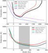 |
Fig. 1. Top panel: temperature stratification in atmospheric models used for non-LTE version of SATIRE-S. The FAL99-C and FAL99-P models (Fontenla et al. 1999) are shown as solid lines and were used to calculate the facular contrast in Eq. (1). The dashed lines show Kurucz solar and stellar models (see U99) used to derive spot contrasts. Bottom panel: comparison of temperature stratifications used in LTE and non-LTE versions of SATIRE-S for calculation of facular contrast. The dashed green curve was derived by modifying the FAL93-P model of Fontenla et al. (1993). The height grids of all models in both panels were offset so that the zero height point in each model corresponds to Rosseland optical depth (calculated in LTE) equal to 2/3. The grey area marks the region of equal temperature difference between quiet Sun and facula in the U99 and FAL99 temperature stratifications (see the Appendix A for discussion). |
The latest version of the NESSY code (Tagirov et al. 2017) has been used to compute the non-LTE intensities in Eq. (1). The code solves the 1D spherically symmetric non-LTE radiative transfer problem for a given temperature and density stratification. The radiative transfer equation and the system of statistical balance equations (SBE) are solved simultaneously for all chemical elements from hydrogen to zinc. The atomic model for each element consists of the ground and first ionised states with varying number of energy levels in the ground state and one energy level in the ionised state. Overall, the atomic model of the code has 114 energy levels (of which 30 are first ionised states), 217 bound-bound transitions and 84 bound-free transitions across the elements included in the model. Once the non-LTE problem is solved, the spectral synthesis block of the code takes the non-LTE energy level populations and employs a linelist compiled from the Kurucz linelist (pers. comm.) and the Vienna Atomic Line Database (VALD, Kupka et al. 1999, 2000) to compute the high resolution (2000 points per nm) spectrum. We have adopted a value of 1.5 km s−1 for the microturbulent velocity during spectral synthesis calculations, which is the same value as was used by Unruh et al. (1999) for facular and quiet Sun spectra. We note that the resulting spectra and, consequently, contrasts of magnetic features depend on the adopted value.
The solar spectrum contains tens of millions of atomic and molecular lines (see, e.g. Shapiro et al. 2019). These lines dominate the SSI variability in the UV, violet, blue, and green spectral domains (Shapiro et al. 2015). Considering all of these lines in non-LTE is presently not feasible. Therefore, a pseudo non-LTE approach is employed in NESSY. In this approach, the code first solves the SBE for all levels of the atomic model described above. Then, the resulting non-LTE populations of the ground and first ionised states of each element, as well as of all hydrogen levels, are passed to the spectral synthesis block of the code. The level populations for all other transitions included in the spectral synthesis are calculated in pseudo non-LTE, that is using the Saha-Boltzmann distribution with respect to the non-LTE populations of the ground and first ionised states. Such treatment allows one to take into account the over-ionisation effects, crucial for proper representation of the spectral profile, in particular in the UV (see, e.g. Short & Hauschildt 2009; Shapiro et al. 2010; Rutten 2019).
We note that molecular lines are currently treated in LTE, which, however, is a reasonable assumption since non-LTE effects in the main molecular bands of the solar spectrum are relatively small (see, e.g. Kleint et al. 2011; Shapiro et al. 2011). A more detailed description of the molecular line treatment in NESSY is given in Shapiro et al. (2010).
The over-ionisation effects and, consequently, the overall intensity distribution of the emergent spectrum of a star (especially in the UV) are influenced by the numerous bound-bound absorptions. This effect is known as line-blanketing (Mihalas 1978, p. 167). One of the reasons for this influence is the change of the ionisation equilibrium state in the stellar photospheric layers due to ionising continuum radiation being blocked by the spectral lines. In the non-LTE case, the ionisation equilibrium is governed by the SBE. In NESSY, the line-blanketing effect on the SBE is included via the LTE opacity distribution function (ODF) procedure. All in all, calculations are performed using the following steps. First, the ODF synthesis is performed in the 100–1000 nm range using LTE populations. In a second step, the ODF is used to calculate non-LTE populations of the ground and first ionised states in the aforementioned atomic model (SBE solution). In the final step, the spectrum is synthesised using the non-LTE populations. For the spectral region considered in this paper (100–1100 nm) this ODF procedure gives the same results as the procedure described by Haberreiter et al. (2008) and Tagirov et al. (2017). The described atomic model, the pseudo non-LTE approach and the ODF procedure for taking the effects of line-blanketing on SBE have been shown to be adequate for representation of the solar spectrum (Shapiro et al. 2010; Tagirov et al. 2017).
3. Results
Figure 2 compares the quiet Sun and active component spectra calculated with NESSY to the spectra calculated with ATLAS9 and to observations. In the SATIRE-S setup used here, the radiative transfer code, the spectral synthesis treatment, and the atmospheres used to derive facular contrasts have all changed. We thus use a sequence of colours (purple, green and red, respectively) to show the effects of these changes step by step. The black, purple and green lines in Figs. 2–4 (and in Fig. A.1) show calculations based on the set of model atmospheres described in U99. Black and purple are for LTE calculations with ATLAS and NESSY and are denoted ATLAS-LTE-U99 and NESSY-LTE-U99 in the text. Spectra and contrasts shown in green are for NESSY calculations in (pseudo) non-LTE and are labelled NESSY-NLTE-U99. The red lines, finally, show NESSY (pseudo) non-LTE calculations for models C (quiet Sun) and P (faculae) from the FAL99 atmosphere set; these are denoted as NESSY-NLTE-FAL99.
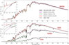 |
Fig. 2. Top panel: comparison of NESSY and ATLAS9 quiet Sun spectra to SIRS WHI observations Woods et al. (2009). NESSY spectra are calculated for three cases. Each case highlights the change in the spectrum at every single step in the progression from ATLAS9 LTE calculation with the set of U99 models to NESSY non-LTE calculation with the FAL99 models. The grey area designates the 1σ uncertainty range of the observations. NESSY and ATLAS9 spectra were convolved with the SIRS WHI spectral resolution. Bottom panel: comparison of facular, umbral and penumbral spectra. The colouring of the curves corresponds to that in the top panel. The three groups of curves on the main panel and the inset correspond, from bottom to top, to umbra, penumbra and facula. NESSY spectra are binned to the ATLAS9 spectral grid. |
The top panel in Fig. 2 compares the synthesised quiet Sun spectra to the SIRS WHI reference quiet Sun spectrum (Woods et al. 2009). The grey area is the 1σ uncertainty range of the observations. The calculated spectra were convolved with the SIRS WHI spectral window (the procedure is the same as in Tagirov et al. 2017).
The inset plot in the top part of Fig. 2 shows that all spectra calculated with the Kurucz quiet Sun model fall below the observed spectrum shortward of about 180 nm. This is explained by the absence of chromospheric layers in that model. The black curve is cut short around 150 nm for the same reason. Technical details of ATLAS9 radiative transfer numerical scheme result in extremely low intensity values for this spectral domain.
The lack of spectral lines in the NESSY-NLTE-FAL99 curves between 125 nm and 180 nm is because all lines in this spectral region, except for the hydrogen Lyman series, are treated in pseudo non-LTE in NESSY (see Sect. 2). These spectral lines form high above the temperature minimum and when treated in pseudo non-LTE the amount of intensity emitted in each of them is erroneously high. To avoid it, in NESSY, the value of the source function for these lines is set to the value of the Planck function at the temperature minimum. This, in turn, leads to insufficient emission when compared to observations. A full non-LTE treatment of these lines is necessary in order for them to appear in the non-LTE spectrum.
Another feature of the red curve is the underestimated Lyα flux. This can be remedied by adjusting the Doppler broadening velocity parameter in the non-LTE block of NESSY (see Sect. 5.2 in Tagirov et al. 2017). However, since the focus of this work was on the verification of the overall SATIRE-S SSI variability profile, such Doppler velocity tuning has not been performed.
Longward of 450 nm the NESSY-NLTE-U99 spectrum (green line) falls below the NESSY-LTE-U99 spectrum (purple) because of the non-LTE increase of H− concentration in the photospheric layers. H− is dissociated mainly by the near-IR photons (Mihalas 1978, p. 102). Increased H− concentration, caused by the visible and near-IR photons escaping the solar atmosphere, leads to a higher H− opacity. Thus, the continuum longward of 450 nm forms at lower photospheric temperatures. The non-LTE H− concentration effect was originally reported by Vernazza et al. (1981) and has been demonstrated for the FAL99 set of models by Shapiro et al. (2010).
The bottom panel of Fig. 2 shows the comparison of ATLAS9 and NESSY spectra of facula, umbra and penumbra. NESSY spectra were binned to the ATLAS9 spectral grid. The three groups of curves in the main panel and inset correspond to umbra (bottom), penumbra (middle) and facula (top), respectively. For wavelengths above 450 nm, the aforementioned H− effect is seen in all three cases. The noticeably lower flux in ATLAS9 umbra calculations between 490 nm and 530 nm is attributed to the opacity from MgH bands, which is not taken into account in NESSY calculations but is significantly overestimated in the old linelists used by Unruh et al. (1999) for their ATLAS9 calculations (see, e.g. Weck et al. 2003).
Figure 2 is concerned with the disc-integrated fluxes. In Fig. 3 we compare ATLAS9 and NESSY quiet Sun centre-to-limb variations (CLV) to the available observations. We plotted the relative deviations of the ATLAS9 and NESSY CLV from Neckel & Labs (1994) fits. All CLV have been normalised to the intensity at the centre of the solar disc. The selection of wavelengths is identical to that used in U99 (see their Fig. 2, bottom panel). NESSY CLV are calculated for the cases shown in Fig. 2. All resulting CLV show comparable deviations from the fits, with NESSY performing somewhat worse at 1047 nm. Close to the limb the agreement of all CLV with observations is limited by the 1D representation of solar atmosphere (Koesterke et al. 2008; Uitenbroek & Criscuoli 2011).
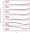 |
Fig. 3. Relative deviations of ATLAS9 and NESSY CLV from CLV fits by Neckel & Labs (1994). The wavelength selection is the same as in Fig. 2 of U99. NESSY CLV are binned to the ATLAS9 spectral grid. The x-axis is the cosine of the heliospheric angle. |
Figure 4 shows the comparison of full-disc relative facular, penumbral and umbral contrasts
 (2)
(2)
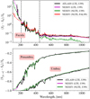 |
Fig. 4. Relative full-disc facular, umbral and penumbral contrasts (Eq. (2)) as calculated with ATLAS9 in LTE for U99 models and with NESSY in LTE and non-LTE for U99 and FAL99 models (faculae only). Each curve is derived from the corresponding curves in Fig. 2 and shows the impact on the relative contrasts produced by the change of code, radiative transfer treatment and the atmospheric model set. Shortward of about 150 nm the black curves are truncated because of the limitations of the ATLAS9 code at these wavelengths. NESSY contrasts are binned to the ATLAS9 spectral grid. The dashed lines designate the spectral domain of similar facular contrasts (see main text). |
calculated with NESSY versus the contrasts calculated with ATLAS9. Here, Sq(λ) is the full disc quiet Sun radiative flux (Eq. (1)) and Sj(λ) is computed analogously for each active feature (i.e. as if the quiet Sun or a given active feature occupied the whole solar disc). Each curve in Fig. 4 is derived from the corresponding curves in Fig. 2, so that one can see the impact on the contrasts from the change of the code, radiative transfer treatment and atmospheric model set.
Figure 4 shows that the spot contrasts hardly changed. The facular contrasts, in turn, differ shortward of the Al I ionisation edge (about 210 nm). In addition, the NESSY-NLTE-U99 facular contrast longward of 450 nm is lower than for the rest of the computations. Shortward of 210 nm the difference between the facular contrasts calculated with the U99 set of models and the FAL99 set is due to the absence of chromospheric layers in the U99 models. Longward of 450 nm the NESSY-NLTE-U99 contrast is shifted downwards from its LTE counterpart due to the non-LTE increase of the H− concentration (see above). This effect is offset by the presence of chromospheric layers in the FAL99 models. Interestingly, all contrasts are remarkably similar in the 210–450 nm domain. The explanation of this is given in Appendix A.
To reconstruct TSI and SSI, we substituted the non-LTE NESSY spectra, calculated with the models shown in the upper panel of Fig. 1, and SDO/HMI filling factors covering the period of solar cycle 24 into Eq. (1). Integrating Eq. (1) over wavelength produces the TSI reconstruction shown in the top panel of Fig. 5 with the red curve. Also shown, in black, are the TSI reconstruction based on the ATLAS9 spectra (computed with the U99 set of models) and the empirically corrected SATIRE-S output (in grey, Yeo et al. 2014, see also the Introduction to this paper for a brief description). The TSI computed in these three cases are hardly distinguishable from each other. We note that the NESSY-NLTE contrasts are slightly higher than the original U99 contrasts in the visible (see Fig. 4), which leads to an increase in their bolometric contrast. As a consequence, the new reconstructions require slightly smaller facular filling factors, so that the fitted value of the Bsat parameter has increased from 267 G given by Yeo et al. (2014) to 346 G.
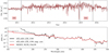 |
Fig. 5. Top panel: TSI calculated with SATIRE-S using SDO/HMI filling factors covering period of solar cycle 24 in combination with NESSY and ATLAS9 spectra (red and black curves, respectively; almost indistinguishable). TSI 1σ uncertainty range as given by the empirically corrected SATIRE-S based on ATLAS9 spectra is shown in grey. The dashed lines designate the periods of minimum (from 3 June 2010 to 2 April 2011) and maximum (from 4 December 2014 to 3 October 2015) solar activity over which the average values of SSI were calculated for computation of SSI variability profile (Eq. (3)) shown in the bottom panel. Bottom panel: relative difference between SSI at activity maximum and minimum versus wavelength (variability profile, Eq. (3)). SSI at minimum and maximum solar activity are averages over the periods marked “min” and “max” (and dashed lines) in the upper panel. The dot represents a negative value. The resolution of all curves is that of the ATLAS9 spectrum (see Sect. 2). Shortward of about 150 nm the black curve is truncated because of ATLAS9 limitations. |
The lower panel of Fig. 5 shows the relative difference between the average values of SSI over the periods of maximum and minimum activity
 (3)
(3)
Here, S(t, λ) is the time-dependent flux as defined by Eq. (1) and the angular brackets represent the averaging over the minimum and maximum time periods indicated in the top panel of Fig. 5 (dates are given in the figure caption).
For wavelengths below 210 nm, the non-LTE SSI variability (red) is much closer to the empirically corrected SATIRE-S values (grey) than the LTE results (shown in black). Above 210 nm all three approaches yield very similar SSI variability. The difference between the non-LTE and LTE SSI variability profiles is readily explained in terms of the contrasts shown in Fig. 4. Since the transition from ATLAS9 LTE to NESSY non-LTE calculations hardly changes the spot contrasts, the difference between the corresponding SSI variabilities is determined by the difference of the facular contrasts prevailing below 210 nm.
4. Summary, conclusions, and outlook
Solar irradiance variability modelling provides important input to models of global climate change (Solanki et al. 2013; Ermolli et al. 2013), and increases our understanding of the place of the Sun among other stars in the context of brightness variability patterns (e.g. Basri et al. 2013; Shapiro et al. 2013, 2014). It also provides a foundation for realistic models of stellar brightness variability required in the field of exoplanet detection (Boisse et al. 2012; Korhonen et al. 2015).
The SATIRE-S model has been highly successful in reproducing the observed TSI and SSI variability (Krivova et al. 2003, 2006; Wenzler et al. 2005, 2006; Ball et al. 2012; Yeo et al. 2014, 2015, 2017a). However, its output below 300 nm has had to be corrected empirically to overcome the limitations of the LTE approximation in this wavelength range (Krivova et al. 2006; Yeo et al. 2014). Due to the long-standing debate on the amplitude of the SSI variability in the spectral range 200 – 400 nm, in particular, the disagreement between the empirical and semi-empirical models (Ermolli et al. 2013; Thuillier et al. 2014; Yeo et al. 2015, 2017a; Egorova et al. 2018), and the importance of this range for climate models (Sukhodolov et al. 2014; Ball et al. 2014a; Maycock et al. 2015, 2016; Ball et al. 2016), this correction reduces the stringency of SATIRE-S results.
To remove the need for such a correction, we have constructed the non-LTE version of SATIRE-S. In this version the ATLAS9 (Kurucz 1992; Castelli & Kurucz 1994) LTE spectra of quiet Sun and active components have been replaced with the non-LTE spectra synthesised with the NESSY code (Tagirov et al. 2017). Additionally, for the quiet Sun and facular contrast terms of Eq. (1), we changed the Kurucz quiet Sun model and the modified FAL93-P model (Fontenla et al. 1993; Unruh et al. 1999), previously used in SATIRE-S, to the corresponding FAL99 models (Fontenla et al. 1999).
We analysed the change of contrasts caused by the use of NESSY and the new set of models (Fig. 4) and compared the non-LTE version of TSI and SSI to the empirically corrected and uncorrected LTE ones for solar cycle 24 (Fig. 5). TSI computed in all three cases are nearly indistinguishable from each other. Comparing SSI we found that below 200 nm the non-LTE version agrees well with the empirically corrected LTE version, although it does not capture the spectral line structure between 125 nm and 180 nm due to the limitations of the NESSY code (see the last paragraph of Sect. 2). Above 200 nm, where the difference between non-LTE and LTE facular contrasts is not as large as below 200 nm, the SSI remains essentially unchanged when the non-LTE approach is employed instead of the empirical correction, except for the two regions around 300 nm and 470 nm, where the agreement between the two is somewhat worse. The empirical correction of the SATIRE-S model computed in LTE is thereby shown to give SSI in line with a non-LTE computation.
In this paper we have presented the non-LTE advancement of the SATIRE-S model. The next step will be the release of non-LTE SATIRE-S with chromospheric lines. In order for this to be accomplished, the lower variability in Lyα and the absence of chromospheric lines between 125 nm and 160 nm in the NESSY code have to be addressed. Apart from that, better 1D semi-empirical models of umbra and penumbra with chromospheric layers have to be created. The recent ALMA observations (Loukitcheva et al. 2017) present an opportunity for the development of such models.
Acknowledgments
We thank Marty Snow for motivating us to carry out this study. We confirm that no funding has been received for it other than from universities, research institutes, and research councils. We thank the International Space Science Institute, Bern, Switzerland for providing financial support and meeting facilities that allowed stimulating discussions (ISSI Team 373 “Towards a Unified Solar Forcing Input to Climate Studies”). The research leading to this paper has received funding from STFC consolidated grants ST/N000838/1 and ST/S000372/1, from the European Research Council under the European Union Horizon 2020 research and innovation programme (grant agreement No. 715947) and the German Federal Ministry of Education and Research (Bundesministerium für Bildung und Forschung) under Project No. 01LG1209A. The SATIRE-S TSI and SSI reconstructions are available at http://www2.mps.mpg.de/projects/sun-climate/data.html. Finally, we thank the referee for their critical assessment of our work and the useful suggestions that helped to improve it significantly.
References
- Aigrain, S., Favata, F., & Gilmore, G. 2004, A&A, 414, 1139 [NASA ADS] [CrossRef] [EDP Sciences] [Google Scholar]
- Austin, J., Tourpali, K., Rozanov, E., et al. 2008, J. Geophys. Res. (Atmos.), 113, D11306 [NASA ADS] [CrossRef] [Google Scholar]
- Ball, W. T., Unruh, Y. C., Krivova, N. A., et al. 2012, A&A, 541, A27 [NASA ADS] [CrossRef] [EDP Sciences] [Google Scholar]
- Ball, W. T., Krivova, N. A., Unruh, Y. C., Haigh, J. D., & Solanki, S. K. 2014a, J. Atmos. Sci., 71, 4086 [NASA ADS] [CrossRef] [Google Scholar]
- Ball, W. T., Mortlock, D. J., Egerton, J. S., & Haigh, J. D. 2014b, J. Space Weather Space Clim., 4, A25 [CrossRef] [EDP Sciences] [Google Scholar]
- Ball, W. T., Haigh, J. D., Rozanov, E. V., et al. 2016, Nat. Geosci., 9, 206 [NASA ADS] [CrossRef] [Google Scholar]
- Basri, G., Walkowicz, L. M., & Reiners, A. 2013, ApJ, 769, 37 [NASA ADS] [CrossRef] [Google Scholar]
- Batalha, N. M. 2014, Proc. Nat. Acad. Sci., 111, 12647 [NASA ADS] [CrossRef] [Google Scholar]
- Boisse, I., Bonfils, X., & Santos, N. C. 2012, A&A, 545, A109 [NASA ADS] [CrossRef] [EDP Sciences] [Google Scholar]
- Brasseur, G., & Solomon, S. 2005, Aeronomy of the Middle Atmosphere: Chemistry and Physics of the Stratosphere and Mesosphere, Atmospheric and Oceanographic Sciences Library (Dordrecht: Springer Netherlands) [Google Scholar]
- Castelli, F., & Kurucz, R. L. 1994, A&A, 281, 817 [NASA ADS] [Google Scholar]
- Desort, M., Lagrange, A. M., Galland, F., Udry, S., & Mayor, M. 2007, A&A, 473, 983 [NASA ADS] [CrossRef] [EDP Sciences] [Google Scholar]
- Egorova, T., Schmutz, W., Rozanov, E., et al. 2018, A&A, 615, A85 [NASA ADS] [CrossRef] [EDP Sciences] [Google Scholar]
- Ermolli, I., Matthes, K., Dudok de Wit, T., et al. 2013, Chem. Phys., 13, 3945 [Google Scholar]
- Fligge, M., Solanki, S. K., & Unruh, Y. C. 2000, A&A, 353, 380 [NASA ADS] [Google Scholar]
- Fontenla, J. M., Avrett, E. H., & Loeser, R. 1993, ApJ, 406, 319 [NASA ADS] [CrossRef] [Google Scholar]
- Fontenla, J., White, O. R., Fox, P. A., Avrett, E. H., & Kurucz, R. L. 1999, ApJ, 518, 480 [NASA ADS] [CrossRef] [Google Scholar]
- Gilliland, R. L., Chaplin, W. J., Dunham, E. W., et al. 2011, ApJS, 197, 6 [NASA ADS] [CrossRef] [Google Scholar]
- Gilliland, R. L., Chaplin, W. J., Jenkins, J. M., Ramsey, L. W., & Smith, J. C. 2015, AJ, 150, 133 [NASA ADS] [CrossRef] [Google Scholar]
- Haberreiter, M., Schmutz, W., & Hubeny, I. 2008, A&A, 492, 833 [NASA ADS] [CrossRef] [EDP Sciences] [Google Scholar]
- Haigh, J. D. 1994, Nature, 370, 544 [NASA ADS] [CrossRef] [Google Scholar]
- Haigh, J. D. 2007, Living Rev. Sol. Phys., 4, 2 [NASA ADS] [Google Scholar]
- Haigh, J. D., Winning, A. R., Toumi, R., & Harder, J. W. 2010, Nature, 467, 696 [NASA ADS] [CrossRef] [PubMed] [Google Scholar]
- Harder, J. W., Fontenla, J. M., Pilewskie, P., Richard, E. C., & Woods, T. N. 2009, Geophys. Res., 36, L07801 [NASA ADS] [Google Scholar]
- Kleint, L., Shapiro, A. I., Berdyugina, S. V., & Bianda, M. 2011, A&A, 536, A47 [NASA ADS] [CrossRef] [EDP Sciences] [Google Scholar]
- Koesterke, L., Allende Prieto, C., & Lambert, D. L. 2008, ApJ, 680, 764 [NASA ADS] [CrossRef] [Google Scholar]
- Kopp, G. 2016, J. Space Weather Space Clim., 6, A30 [Google Scholar]
- Korhonen, H., Andersen, J. M., Piskunov, N., et al. 2015, MNRAS, 448, 3038 [NASA ADS] [CrossRef] [EDP Sciences] [Google Scholar]
- Krivova, N. A., Solanki, S. K., Fligge, M., & Unruh, Y. C. 2003, A&A, 399, L1 [NASA ADS] [CrossRef] [EDP Sciences] [Google Scholar]
- Krivova, N. A., Solanki, S. K., & Floyd, L. 2006, A&A, 452, 631 [NASA ADS] [CrossRef] [EDP Sciences] [Google Scholar]
- Krivova, N. A., Solanki, S. K., & Unruh, Y. C. 2011, J. Atmos. Solar-Terr. Phys., 73, 223 [NASA ADS] [CrossRef] [Google Scholar]
- Kupka, F., Piskunov, N., Ryabchikova, T. A., Stempels, H. C., & Weiss, W. W. 1999, A&AS, 138, 119 [NASA ADS] [CrossRef] [EDP Sciences] [MathSciNet] [PubMed] [Google Scholar]
- Kupka, F. G., Ryabchikova, T. A., Piskunov, N. E., Stempels, H. C., & Weiss, W. W. 2000, Baltic Astron., 9, 590 [Google Scholar]
- Kurucz, R. L. 1992, Rev. Mex. Astron. Astrofis., 23, 45 [Google Scholar]
- Kurucz, R. L. 1993, ATLAS9 Stellar Atmosphere Programs and 2 km/s grid. Kurucz CD-ROM No. 13 (Smithsonian Astrophysical Observatory) [Google Scholar]
- Lagrange, A. M., Desort, M., & Meunier, N. 2010, A&A, 512, A38 [NASA ADS] [CrossRef] [EDP Sciences] [Google Scholar]
- Loukitcheva, M. A., Iwai, K., Solanki, S. K., White, S. M., & Shimojo, M. 2017, ApJ, 850, 35 [NASA ADS] [CrossRef] [Google Scholar]
- Maycock, A. C., Ineson, S., Gray, L. J., et al. 2015, J. Geophys. Res. (Atmos.), 120, 9043 [NASA ADS] [CrossRef] [Google Scholar]
- Maycock, A. C., Matthes, K., Tegtmeier, S., Thiéblemont, R., & Hood, L. 2016, Atmos. Chem. Phys., 16, 10021 [NASA ADS] [CrossRef] [Google Scholar]
- McClintock, W. E., Rottman, G. J., & Woods, T. N. 2005, Sol. Phys., 230, 225 [NASA ADS] [CrossRef] [Google Scholar]
- Mihalas, D. 1978, Stellar Atmospheres, 2nd edn. (San Francisco, WH: Freeman and Co.) [Google Scholar]
- Mitchell, D. M., Misios, S., Gray, L. J., et al. 2015, Q. J. R. Meteorol. Soc., 141, 2390 [NASA ADS] [CrossRef] [Google Scholar]
- Neckel, H., & Labs, D. 1994, Sol. Phys., 153, 91 [NASA ADS] [CrossRef] [Google Scholar]
- Pont, F., Knutson, H., Gilliland, R. L., Moutou, C., & Charbonneau, D. 2008, MNRAS, 385, 109 [NASA ADS] [CrossRef] [Google Scholar]
- Rottman, G. 2005, Sol. Phys., 230, 7 [NASA ADS] [CrossRef] [Google Scholar]
- Rutten, R. J. 2019, Sol. Phys., submitted [arXiv:1908.04624] [Google Scholar]
- Saar, S. H., & Donahue, R. A. 1997, ApJ, 485, 319 [NASA ADS] [CrossRef] [Google Scholar]
- Shapiro, A. I., Schmutz, W., Schoell, M., Haberreiter, M., & Rozanov, E. 2010, A&A, 517, A48 [NASA ADS] [CrossRef] [EDP Sciences] [Google Scholar]
- Shapiro, A. I., Fluri, D. M., Berdyugina, S. V., Bianda, M., & Ramelli, R. 2011, A&A, 529, A139 [NASA ADS] [CrossRef] [EDP Sciences] [Google Scholar]
- Shapiro, A. I., Schmutz, W., Cessateur, G., & Rozanov, E. 2013, A&A, 552, A114 [NASA ADS] [CrossRef] [EDP Sciences] [Google Scholar]
- Shapiro, A. I., Solanki, S. K., Krivova, N. A., et al. 2014, A&A, 569, A38 [Google Scholar]
- Shapiro, A. I., Solanki, S. K., Krivova, N. A., Tagirov, R. V., & Schmutz, W. K. 2015, A&A, 581, A116 [NASA ADS] [CrossRef] [EDP Sciences] [Google Scholar]
- Shapiro, A. I., Peter, H., & Solanki, S. K. 2019, Chapter 3 – The Sun’s Atmospher (Amsterdam: Elsevier), 59 [Google Scholar]
- Short, C. I., & Hauschildt, P. H. 2009, ApJ, 691, 1634 [NASA ADS] [CrossRef] [Google Scholar]
- Solanki, S. K. 2003, A&A Rev., 11, 153 [NASA ADS] [CrossRef] [Google Scholar]
- Solanki, S. K., Krivova, N. A., & Haigh, J. D. 2013, ARA&A, 51, 311 [NASA ADS] [CrossRef] [Google Scholar]
- Soukharev, B. E., & Hood, L. L. 2006, J. Geophys. Res. (Atmos.), 111, D20314 [Google Scholar]
- Sukhodolov, T., Rozanov, E., Shapiro, A. I., et al. 2014, Geosci. Model Dev., 7, 2859 [NASA ADS] [CrossRef] [Google Scholar]
- Tagirov, R. V., Shapiro, A. I., & Schmutz, W. 2017, A&A, 603, A27 [NASA ADS] [CrossRef] [EDP Sciences] [Google Scholar]
- Thuillier, G., Schmidtke, G., Erhardt, C., et al. 2014, Sol. Phys., 289, 4433 [NASA ADS] [CrossRef] [Google Scholar]
- Uitenbroek, H., & Criscuoli, S. 2011, ApJ, 736, 69 [NASA ADS] [CrossRef] [Google Scholar]
- Unruh, Y. C., Solanki, S. K., & Fligge, M. 1999, A&A, 345, 635 [NASA ADS] [Google Scholar]
- Unruh, Y. C., Ball, W. T., & Krivova, N. A. 2012, Surv. Geophys., 33, 475 [Google Scholar]
- Vernazza, J. E., Avrett, E. H., & Loeser, R. 1981, ApJS, 45, 635 [NASA ADS] [CrossRef] [Google Scholar]
- Weck, P. F., Schweitzer, A., Stancil, P. C., Hauschildt, P. H., & Kirby, K. 2003, ApJ, 582, 1059 [NASA ADS] [CrossRef] [Google Scholar]
- Wenzler, T., Solanki, S. K., & Krivova, N. A. 2005, A&A, 432, 1057 [NASA ADS] [CrossRef] [EDP Sciences] [Google Scholar]
- Wenzler, T., Solanki, S. K., Krivova, N. A., & Fröhlich, C. 2006, A&A, 460, 583 [NASA ADS] [CrossRef] [EDP Sciences] [Google Scholar]
- Woods, T. N., Chamberlin, P. C., Harder, J. W., et al. 2009, Geophys. Res., 36, l01101 [Google Scholar]
- Yeo, K. L., Krivova, N. A., Solanki, S. K., & Glassmeier, K. H. 2014, A&A, 570, A85 [NASA ADS] [CrossRef] [EDP Sciences] [Google Scholar]
- Yeo, K. L., Ball, W. T., Krivova, N. A., et al. 2015, J. Geophys. Res. (Space Phys.), 120, 6055 [NASA ADS] [CrossRef] [Google Scholar]
- Yeo, K. L., Krivova, N. A., & Solanki, S. K. 2017a, J. Geophys. Res. (Space Phys.), 122, 3888 [Google Scholar]
- Yeo, K. L., Solanki, S. K., Norris, C. M., et al. 2017b, Phys. Rev. Lett., 119, 1102 [Google Scholar]
Appendix A: Analysis of the contrast similarity in the 210 nm to 450 nm spectral domain
The similarity of the contrasts between 210 nm and 450 nm shown in Fig. 4 can be interpreted by considering the formation heights of the fluxes. Fig. A.1 shows the formation height of full-disc quiet Sun and facular fluxes calculated with NESSY for the LTE-U99 and NLTE-FAL99 cases. The formation heights were shifted in the same way as the height grids in Fig. 1, so that there is a one-to-one correspondence between the formation heights plotted in Fig. A.1 and the temperature structures in Fig. 1. The idea behind using Figs. 1 and A.1 for the interpretation of the contrasts similarity is to associate the contrasts with the temperature differences at the corresponding formation heights. Strictly speaking such an association is only valid under the assumption of LTE, when the source function is equal to the Planck function and thus is defined by the local temperature. However, it should be accurate enough for our illustrative purposes. In particular, we note that the effect of over-ionisation on spectral lines only changes their opacity, but not their source function.
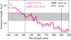 |
Fig. A.1. Formation height of full-disc quiet Sun and facular fluxes computed with NESSY for LTE-U99 and NLTE-FAL99 cases. The intermediate case (NLTE-U99) has been omitted for visual clarity. The vertical dotted lines refer to the same spectral domain as in the top panel of Fig. 4. The grey area designates the region, where the temperature differences between quiet Sun and facula in the U99 and FAL99 atmospheric model sets are equal (see Fig. 1, bottom panel). The high resolution formation heights (2000 points per nm) were weighted with the corresponding intensity, averaged over 1 nm intervals and then shifted in the same way as the height grids in Fig. 1. |
We can see that the formation heights are decreasing and in the NLTE-FAL99 case they are the same for the quiet Sun and faculae almost everywhere. It means that the NESSY-NLTE-FAL99 contrast is given by the difference between the corresponding quiet-Sun and facular temperatures in Fig. 1 at each height. According to Fig. 1, down to the zero height point, this temperature difference and, consequently, the contrast diminish. In the LTE-U99 case, the formation heights are equal starting from 210 nm up to approximately 300 nm. In this range they fall into the grey area, which designates the region of (almost) equal temperature difference between quiet Sun and facula in the U99 and FAL99 sets (see Fig. 1, bottom panel). Hence, from 210 nm to 300 nm the LTE-U99 formation temperature difference and contrast are similar to the NLTE-FAL99 case. Between 300 nm and 450 nm the spectrum forms in the regions where the U99 temperature difference between quiet Sun and facula decreases faster than in the FAL99 case. However, the formation height in the U99 facula becomes greater than in the quiet Sun, thus compensating for the faster decrease and preserving the equality of LTE-U99 and NLTE-FAL99 contrasts up to 450 nm.
All Figures
|
Fig. 1. Top panel: temperature stratification in atmospheric models used for non-LTE version of SATIRE-S. The FAL99-C and FAL99-P models (Fontenla et al. 1999) are shown as solid lines and were used to calculate the facular contrast in Eq. (1). The dashed lines show Kurucz solar and stellar models (see U99) used to derive spot contrasts. Bottom panel: comparison of temperature stratifications used in LTE and non-LTE versions of SATIRE-S for calculation of facular contrast. The dashed green curve was derived by modifying the FAL93-P model of Fontenla et al. (1993). The height grids of all models in both panels were offset so that the zero height point in each model corresponds to Rosseland optical depth (calculated in LTE) equal to 2/3. The grey area marks the region of equal temperature difference between quiet Sun and facula in the U99 and FAL99 temperature stratifications (see the Appendix A for discussion). |
| In the text | |
|
Fig. 2. Top panel: comparison of NESSY and ATLAS9 quiet Sun spectra to SIRS WHI observations Woods et al. (2009). NESSY spectra are calculated for three cases. Each case highlights the change in the spectrum at every single step in the progression from ATLAS9 LTE calculation with the set of U99 models to NESSY non-LTE calculation with the FAL99 models. The grey area designates the 1σ uncertainty range of the observations. NESSY and ATLAS9 spectra were convolved with the SIRS WHI spectral resolution. Bottom panel: comparison of facular, umbral and penumbral spectra. The colouring of the curves corresponds to that in the top panel. The three groups of curves on the main panel and the inset correspond, from bottom to top, to umbra, penumbra and facula. NESSY spectra are binned to the ATLAS9 spectral grid. |
| In the text | |
|
Fig. 3. Relative deviations of ATLAS9 and NESSY CLV from CLV fits by Neckel & Labs (1994). The wavelength selection is the same as in Fig. 2 of U99. NESSY CLV are binned to the ATLAS9 spectral grid. The x-axis is the cosine of the heliospheric angle. |
| In the text | |
|
Fig. 4. Relative full-disc facular, umbral and penumbral contrasts (Eq. (2)) as calculated with ATLAS9 in LTE for U99 models and with NESSY in LTE and non-LTE for U99 and FAL99 models (faculae only). Each curve is derived from the corresponding curves in Fig. 2 and shows the impact on the relative contrasts produced by the change of code, radiative transfer treatment and the atmospheric model set. Shortward of about 150 nm the black curves are truncated because of the limitations of the ATLAS9 code at these wavelengths. NESSY contrasts are binned to the ATLAS9 spectral grid. The dashed lines designate the spectral domain of similar facular contrasts (see main text). |
| In the text | |
|
Fig. 5. Top panel: TSI calculated with SATIRE-S using SDO/HMI filling factors covering period of solar cycle 24 in combination with NESSY and ATLAS9 spectra (red and black curves, respectively; almost indistinguishable). TSI 1σ uncertainty range as given by the empirically corrected SATIRE-S based on ATLAS9 spectra is shown in grey. The dashed lines designate the periods of minimum (from 3 June 2010 to 2 April 2011) and maximum (from 4 December 2014 to 3 October 2015) solar activity over which the average values of SSI were calculated for computation of SSI variability profile (Eq. (3)) shown in the bottom panel. Bottom panel: relative difference between SSI at activity maximum and minimum versus wavelength (variability profile, Eq. (3)). SSI at minimum and maximum solar activity are averages over the periods marked “min” and “max” (and dashed lines) in the upper panel. The dot represents a negative value. The resolution of all curves is that of the ATLAS9 spectrum (see Sect. 2). Shortward of about 150 nm the black curve is truncated because of ATLAS9 limitations. |
| In the text | |
|
Fig. A.1. Formation height of full-disc quiet Sun and facular fluxes computed with NESSY for LTE-U99 and NLTE-FAL99 cases. The intermediate case (NLTE-U99) has been omitted for visual clarity. The vertical dotted lines refer to the same spectral domain as in the top panel of Fig. 4. The grey area designates the region, where the temperature differences between quiet Sun and facula in the U99 and FAL99 atmospheric model sets are equal (see Fig. 1, bottom panel). The high resolution formation heights (2000 points per nm) were weighted with the corresponding intensity, averaged over 1 nm intervals and then shifted in the same way as the height grids in Fig. 1. |
| In the text | |
Current usage metrics show cumulative count of Article Views (full-text article views including HTML views, PDF and ePub downloads, according to the available data) and Abstracts Views on Vision4Press platform.
Data correspond to usage on the plateform after 2015. The current usage metrics is available 48-96 hours after online publication and is updated daily on week days.
Initial download of the metrics may take a while.