| Issue |
A&A
Volume 631, November 2019
|
|
|---|---|---|
| Article Number | A99 | |
| Number of page(s) | 18 | |
| Section | The Sun | |
| DOI | https://doi.org/10.1051/0004-6361/201834083 | |
| Published online | 29 October 2019 | |
Superstrong photospheric magnetic fields in sunspot penumbrae
1
Max-Planck-Institut für Sonnensystemforschung, Justus-von-Liebig-Weg 3, 37077 Göttingen, Germany
2
Instituto de Astrofísica de Andalucía (IAA-CSIC), Apdo. 3004, 18080 Granada, Spain
e-mail: This email address is being protected from spambots. You need JavaScript enabled to view it.
3
High Altitude Observatory, NCAR, PO Box 3000 Boulder, CO 80307, USA
4
School of Space Research, Kyung Hee University, Yongin 446-701 Gyeonggi, Republic of Korea
Received:
13
August
2018
Accepted:
23
September
2019
Abstract
Context. Recently, there have been some reports of unusually strong photospheric magnetic fields (which can reach values of over 7 kG) inferred from Hinode SOT/SP sunspot observations within penumbral regions. These superstrong penumbral fields are even larger than the strongest umbral fields on record and appear to be associated with supersonic downflows. The finding of such fields has been controversial since they seem to show up only when spatially coupled inversions are performed.
Aims. Here, we investigate and discuss the reliability of those findings by studying in detail observed spectra associated with particularly strong magnetic fields at the inner edge of the penumbra of active region 10930.
Methods. We applied classical diagnostic methods and various inversions with different model atmospheres to the observed Stokes profiles in two selected pixels with superstrong magnetic fields, and compared the results with a magnetohydrodynamic simulation of a sunspot whose penumbra contains localized regions with strong fields (nearly 5 kG at τ = 1) associated with supersonic downflows.
Results. The different inversions provide different results: while the SPINOR 2D inversions consider a height-dependent single-component model and return B > 7 kG and supersonic positive vLOS (corresponding to a counter-Evershed flow), height-dependent two-component inversions suggest the presence of an umbral component (almost at rest) with field strengths ∼4 − 4.2 kG and a penumbral component with vLOS ∼ 16 − 18 km s−1 and field strengths up to ∼5.8 kG. Likewise, height-independent two-component inversions find a solution for an umbral component and a strongly redshifted (vLOS ∼ 15 − 17 km s−1) penumbral component with B ∼ 4 kG. According to a Bayesian information criterion, the inversions providing a better balance between the quality of the fits and the number of free parameters considered by the models are the height-independent two-component inversions, but they lie only slightly above the SPINOR 2D inversions. Since it is expected that the physical parameters all display considerable gradients with height, as supported by magnetohydrodynamic (MHD) sunspot simulations, the SPINOR 2D inversions are the preferred ones.
Conclusions. According to the MHD sunspot simulation analyzed here, the presence of counter-Evershed flows in the photospheric penumbra can lead to the necessary conditions for the observation of ∼5 kG fields at the inner penumbra. Although a definite conclusion about the potential existence of fields in excess of 7 kG cannot be given, their nature could be explained (based on the simulation results) as the consequence of the extreme dynamical effects introduced by highly supersonic counter-Evershed flows (vLOS > 10 km s−1 and up to ∼30 km s−1 according to SPINOR 2D). The latter are much faster and more compressive downflows than those found in the MHD simulations and therefore could lead to field intensification up to considerably stronger fields. Also, a lower gas density would lead to a deeper depression of the τ = 1 surface, making possible the observation of deeper-lying stronger fields. The superstrong magnetic fields are expected to be nearly force-free, meaning that they can attain much larger strengths than expected when considering only balance between magnetic pressure and the local gas pressure.
Key words: Sun: photosphere / sunspots / Sun: magnetic fields
© A. Siu-Tapia et al. 2019
 Open Access article, published by EDP Sciences, under the terms of the Creative Commons Attribution License (http://creativecommons.org/licenses/by/4.0), which permits unrestricted use, distribution, and reproduction in any medium, provided the original work is properly cited.
Open Access funding provided by Max Planck Society.
1. Introduction
Sunspots are the largest concentrations of magnetic flux on the solar surface and, due to the significant suppression of the convective motions caused by the strong fields, they are seen as dark regions on the photosphere. The various brightness levels observed in sunspots indicate differences in temperature, and therefore different magnetic regimes. Such a relation between brightness or temperature and magnetic field strength in the photosphere has been extensively studied (e.g., Lites et al. 1990; Solanki 1993; Keppens & Martínez Pillet 1996; Mathew et al. 2003, 2004; Tiwari et al. 2015).
The strongest magnetic fields in sunspots are generally found within their central dark regions or umbrae, where the field is closely vertical with typical strengths between 2.5 and 4 kG (e.g., Livingston 2002). The largest field strength ever recorded within an umbral region is nearly 6.1 kG (Livingston et al. 2006), but an even larger value (above 6.2 kG) was recently reported by Okamoto & Sakurai (2018), and was observed in a light bridge. Moreover, field strengths in excess of 7 kG have been found within sunspot penumbrae (van Noort et al. 2013; Siu-Tapia et al. 2017). Penumbrae are the brighter regions partially or completely surrounding umbrae and where the magnetic field is filamentary, strongly inclined, and generally weaker than in the umbrae; typically the field varies from about 1.5–2.5 kG at the inner penumbral boundary to 0.5–1 kG towards the outer boundary (e.g., Lites et al. 1990; Skumanich et al. 1994; Westendorp Plaza et al. 2001).
Sunspot penumbrae are additionally characterized by a gas outflow with speeds of several kilometers per second, the so-called Evershed flow (EF; Evershed 1909), which is directed along the penumbral filaments, that is, along the bright elongated channels with more inclined fields within the penumbra itself. Tiwari et al. (2013), in a detailed analysis of the penumbral fine structure, found that the EF has its sources in hot upflows that occur at the inner endpoints of the penumbral filaments (heads) and part of it sinks in concentrated cooler downflows that occur at the outer endpoints (tails) where the magnetic field bends over vertically and displays a strengthening of about 1.5–2.5 kG on average, meaning that it can reach up to 3.5 kG in individual tails.
The superstrong penumbral fields reported by van Noort et al. (2013, field strengths reaching up to 7.5 kG) were observed in some tails of complex penumbral filaments, namely those with a single tail but with more than one head, near the penumbral periphery in supersonic downflow areas (estimated line-of-sight velocities of up to 22 km s−1). Such values were inferred by a sophisticated inversion technique that takes into account the spatial coupling between the pixels of the observed image when considering the instrumental effects that cause the image degradation (SPINOR 2D; van Noort 2012; van Noort et al. 2013).
In contrast, the superstrong fields reported by Siu-Tapia et al. (2017, fields stronger than 7 kG based on SPINOR 2D inversions) were observed in the tails of inverted penumbral filaments carrying a counter-EF (CEF), that is, a gas inflow towards the sunspot umbra at photospheric heights, near the inner penumbral boundary. Unlike in van Noort et al. (2013) and Tiwari et al. (2013), Siu-Tapia et al. (2017) considered the outer endpoint of the CEF-carrying filaments to be heads, since at such places the sources of the CEF were found; and the inner endpoints of the CEF-carrying filaments to be tails, where the sinks of such flow were observed. Therefore, they found on average field strength of ∼4.5 kG (when excluding all those fields in excess of 7 kG) at the tails of the CEF-carrying filaments. Such superstrong penumbral fields were also found to be associated with the supersonic downflows occurring at the sinks of the CEF.
The superstrong penumbral fields reported by both van Noort et al. (2013) and Siu-Tapia et al. (2017) are unusual and are even stronger than the strongest umbral fields found by Livingston et al. (2006) of ∼6.1 kG. Moreover, in both studies, spatially coupled inversions were employed and therefore the reality of these extraordinary field strengths needs to be confirmed with other techniques. The existence of field strengths in excess of 7 kG possibly has an impact on the approximations made by the inversion code, which can lead to errors in the density stratifications if the non-vertical field components are significant, and therefore in the atmospheric stratifications of the physical parameters inferred by the code. Hence, the reliability of the inversion results for such peculiar pixels needs to be tested.
This work is aimed at discussing the reliability of those penumbral fields in excess of 7 kG reported by Siu-Tapia et al. (2017) concentrated at the inner boundary of the penumbra of the main sunspot in active region (AR) 10930. Here, we examine the reality of such findings by applying some classical diagnostic methods and various inversion techniques with different model atmospheres to the Stokes profiles observed with the spectropolarimeter (SP) of the Solar Optical Telescope (SOT) onboard Hinode. Finally, since the mere possibility of such superstrong fields in sunspots leads to the question of the necessary physical conditions for their appearance, we analyze the physical structure of a sunspot magnetohydrodynamic (MHD) simulation with CEFs which was reported by Rempel (2015); see also Siu-Tapia et al. (2018).
This work is organized as follows: in Sect. 2 we describe our data and inversion technique. In Sect. 3, we describe the results obtained with the SPINOR 2D inversion code. In Sect. 4, some classical diagnostic methods are applied to peculiar pixels with extreme spectra. In Sect. 5, various inversions with different model atmospheres are considered. The results are presented in Sect. 6. In Sect. 7, we compare the observations with MHD sunspot simulations and study the mechanisms that can amplify the magnetic field in the penumbra. Finally, in Sect. 8 we discuss our results and draw our conclusions.
2. Observations and spatially coupled inversions
For this study we use the spectropolarimetric observations of AR NOAA 10930 from the Hinode SOT/SP instrument (Lites et al. 2001; Lites & Akin 2013), which simultaneously measures the full Stokes profiles of a pair of absorption lines of Fe I that are formed in the lower solar photosphere with central wavelengths at 6301.5 and 6302.5 Å (and effective Landé factors gL = 1.67 and 2.49, respectively).
The SP instrument scanned the main sunspot in AR 10930 (whose umbra displayed a negative magnetic polarity) on Dec 8 2006 at an heliocentric angle of ∼47° while operating in normal mode, that is, using an exposure time of 4.8 s per slit position and a spatial sampling of 0.16″. These observations were corrected for dark current, flat field, orbital drift, and instrumental cross-talk by reducing the raw data with Interactive Data Language (IDL) routines of the Solar-Soft package (Lites & Ichimoto 2013).
As described by Siu-Tapia et al. (2017), the atmospheric properties of the main sunspot in AR 10930 were derived by inverting the observed Stokes profiles with the SPINOR 2D inversion code (van Noort 2012; van Noort et al. 2013), which is the spatially coupled version of the SPINOR inversion code (Frutiger 2000), based on the STOPRO routines (Solanki 1987) that solve the radiative transfer equations for polarized light.
The method is able to invert 2D maps of spectropolarimetric data that have been degraded spatially in a known way (information that is contained in the point-spread function (PSF) of the telescopes). The code is then able to use the information contained in the spectral dimension and the known spatial degradation properties to constrain a parameterization of the atmosphere over the whole field of view (FOV). The image degradation is applied to the solution rather than by deconvolving the original data themselves (the classical approach), while the code performs a coupled inversion of all the pixels simultaneously.
According to van Noort (2012), the spatially coupled inversion method is stable to oversampled data and produces an inversion result with a resolution up to the resolution limit of the telescope. To be able to reach the diffraction limit of Hinode SOT, we oversampled all Stokes maps by a factor two, to 0.08″, following van Noort et al. (2013). Thus, by considering a spatial grid that is denser than the original data and by employing a single-component atmospheric model per pixel, the inverted atmospheric parameters returned by the code correspond to the best fits to the Stokes profiles once the blurring effect of the PSF of the telescope has been taken into account. This significantly improves the spatial resolution, allowing structures at the diffraction limit of the telescope to be properly resolved.
For the SPINOR 2D inversions used in this work (cf. Siu-Tapia et al. 2017), all the atmospheric free parameters were initially defined at three optical depth nodes, placed at log(τ) = − 2, −0.8, and 0. This set of optical depth nodes was shown to work well for the inversion of Hinode/SP observations of sunspots by Siu-Tapia et al. (2017). At each of the three chosen nodes, the temperature T, magnetic field strength B, field inclination relative to the line-of-sight γLOS, field azimuth ϕ, line-of-sight velocity vLOS, and a microturbulent velocity vMIC were fitted, leading to 18 free parameters in total.
In Fig. 1, the response functions (RFs) of Stokes I and V to the magnetic field B are plotted as functions of wavelength and optical depth for the pair of Fe I absorption lines at 6301.5 and 6302.5 Å. To compute these RFs we used the atmospheric parameters retrieved by SPINOR 2D inversions (see Table 2) in a penumbral pixel with superstrong field (labeled as LFP 1 and marked with a blue plus symbol in Fig. 3a). These plots show that the selected nodes at log(τ) = 0, −0.8 and −2 for performing our inversions all formally lie within the formation region of the lines. In particular, the lowest node at log(τ) = 0 is also sensitive to the magnetic field changes, which means that information about the magnetic field at this node is available for the analyzed wavelength range.
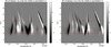 |
Fig. 1. Normalized response function of Stokes I (left) and Stokes V (right) to the magnetic field B, multiplied by 1/ΔτC[10−5 G−1], for the pair of Fe I absorption lines at 6301.5 and 6302.5 Å in the atmosphere inferred by the SPINOR 2D inversions for the penumbral pixel marked with a blue plus symbol in Fig. 3a. Some physical parameters for such an atmosphere are presented in Table 2. The horizontal dashed lines indicate the selected nodes for the SPINOR 2D inversion: log(τ) = 0, −0.8 and −2. |
3. Magnetic and velocity field of the sunspot as inferred by SPINOR 2D
As reported by Siu-Tapia et al. (2017), the SPINOR 2D inversions return very large magnetic field strengths, B ≥ 5 kG at all three height nodes (log(τ) = − 2.0, −0.8 and 0) in the inner center-side penumbra of the main sunspot in AR 10930 (see field strength map in Fig. 2a for the height node at log(τ) = 0 only). Such strong magnetic fields are located at places that coincide with supersonic sinks of the CEF (see Fig. 2b and Figs. 3 and 5 in Siu-Tapia et al. 2017). These are among the largest field strengths ever observed in penumbral environments (see also van Noort et al. 2013).
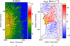 |
Fig. 2. Portion of the (center-side) penumbra of the main sunspot in AR 10930 (cf. Fig. 5 in Siu-Tapia et al. (2017)). Panel a: map of the magnetic field strength at log(τ) = 0, as inferred with SPINOR 2D inversions. The arrow points towards the solar-disk center. Panel b: line-of-sight velocity as inferred with SPINOR 2D inversions at log(τ) = 0. Positive values (red-to-yellow colors) indicate plasma motions away from the observer, while negative values (blue colors) indicate motions towards the observer. Solid and dashed black contour lines were placed at Ic/IQS = 0.26 and Ic/IQS = 0.94, respectively. The large penumbral sector where red-to-yellow colors dominate harbors a fast counter-EF which supersonically sinks (with speeds larger than 12 km s−1) near the inner penumbral boundary (Siu-Tapia et al. 2017). The color-bar scales have been saturated. |
In particular, field strengths above 7 kG (whiter regions near the inner penumbral boundary in Fig. 2a) are even larger than the largest umbral fields found by Livingston et al. (2006) of ∼6.1 kG, who also found that only a very small fraction of sunspots (around 0.2% in a nine-decade record of ∼32 000 sunspots) have umbral fields stronger than 4 kG.
The scatter-plot in Fig. 3b shows the SPINOR 2D inversion results for the magnetic field inclination angle in the local-reference-frame (LRF) after the azimuthal disambiguation was resolved with the Non-Potential Magnetic Field Computation method (NPFC; Georgoulis 2005) versus the line-of-sight (LOS) velocity at log(τ) = 0, for all the 226 pixels where the SPINOR 2D inversions return B ≥ 7 kG (hereafter “large field pixels” (LFPs), yellow markers in Fig. 3a).
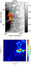 |
Fig. 3. Panel a: normalized continuum intensity map as observed by the Hinode SOT/SP in AR 10930. The red markers indicate the location of 845 pixels where the SPINOR 2D inversions return B ≥ 5 kG at log(τ) = 0, of which 226 harbor fields larger than 7 kG at log(τ) = 0 (yellow markers, also named in the text such as large-field-pixels or LFPs). The blue markers highlight the location of two LFPs (“+”: LFP 1, “×”: LFP 2) selected to test the robustness of our inversion solutions (see text). The arrow points towards the solar-disk center. Panel b: scatter plot of the magnetic field inclination in the local reference frame γLRF (after removal of the field azimuth ambiguity through the NPFC method) vs. the line-of-sight velocity vLOS, from SPINOR 2D at log(τ) = 0, for the 226 LFPs. |
Most of the LFPs (see main population in Fig. 3b) appear associated with supersonic LOS velocities, i.e., around vLOS = 10 km s−1 (the sound speed is around Cs ∼ 5 − 8 km s−1 in penumbrae, e.g., van Noort et al. 2013) and even higher than 20 km s−1 in some pixels. The peak of the LFPs distribution occurs near γLRF = 140°.
Therefore, according to the SPINOR 2D inversions, the LFPs are of umbral polarity (which is negative) with a large longitudinal component and, under the assumption of field-aligned flows, they contain supersonic downflows at log(τ) = 0. See Siu-Tapia et al. (2017) for more details on their brightness and thermal structure.
4. Analysis: Zeeman splitting and center-of-gravity methods
Most of the LFPs inferred by the SPINOR 2D inversions in AR 10930 are located at or close to the umbral/penumbral boundary of the penumbral region hosting a CEF (cf. Figs. 3 and 5 in Siu-Tapia et al. 2017), and display very complex Stokes profiles. Figure 4 shows the observed Stokes profiles (black dashed curves) from two selected LFPs. The locations of the selected LFPs are marked with a blue plus symbol and cross in Fig. 3a (“+”: pixel 1, “×”: pixel 2). All Stokes parameters in these LFPs exhibit large asymmetries and the Stokes V profiles display more than two lobes. Their best fits from SPINOR 2D are not nearly as good as in most of the penumbral pixels (see Fig. 2 in Siu-Tapia et al. 2017). It is noticeable that the continuum intensity and the Stokes V profiles are only imperfectly reproduced in both examples (see also orange curves in Fig. 7).
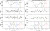 |
Fig. 4. Observed Stokes profiles (dashed curves) in two pixels (left: pixel 1, right: pixel 2) located at the inner penumbra of the CEF region (see blue crosses on maps displayed in Fig. 3a). From top to bottom: Stokes I, Q, U and V. The vertical lines in Stokes I and V panels indicate the position of the λ− (blue) and λ+ (red) used to calculate the magnetic field strength with three different methods (see the main text for a description of the methods): the solid lines in the Stokes V panels show the splitting derived from Method 1; the solid lines in the Stokes I panels correspond to the line splitting obtained with Method 2; and, the dashed lines in both I and V panels indicate the splitting derived from Method 3. The vertical dashed green line shows the wavelength position used to separate the two Fe I lines. |
As a very simple alternative estimation of the field strength in the selected LFPs, we compute the magnetic field strength directly from the splitting of the two observed Fe I line profiles at 6301.5 Å (line 1) and 6302.5 Å (line 2), using the Zeeman splitting formula:
 (1)
(1)
where λ0 is the central wavelength of the line, λ± are the centroids of the right and left circularly polarized line components (σ-components), m and e are the electron mass and charge, gL is the effective Landé factor of the transition (gL = 1.67 for line 1 and gL = 2.5 for line 2), and c is the speed of light. Given the huge field strengths inferred by the SPINOR 2D inversions, the Zeeman splitting should be complete, meaning that this approach is expected to prove the inversion results in case the super-strong fields are real. However, the Zeeman splitting approach can be misleading if there are strong gradients with height or multiple components in the resolution element. A strong magnetic field near optical depth unity which rapidly decreases with height might not display a complete Zeeman splitting in the profiles but very broad wings of the Stokes I and V profiles.
The critical point about using Eq. (1) is determining λ− and λ+ due to the large asymmetries observed in all four Stokes profiles from the LPF. We use three ways: Method (1) Selecting λ− where Stokes V takes on the largest negative value in the blue wing of the corresponding line, and λ+ where Stokes V is largest in its red wing. Method (2) Placing λ− and λ+ where the two deepest minima of Stokes I away from the central wavelength are found (using line 2 only, since line 1 is insufficiently split). Method (3) Applying the center-of-gravity (COG) method (Semel 1967, 1970; Rees & Semel 1979; Cauzzi et al. 1993), in which  , where
  are the center of gravity wavelengths of the centroids of the right and left circularly polarized components, respectively, of the corresponding line, that is:
 (2)
(2)
The position of  and the wavelengths delimiting the integration intervals in Eq. (2) for each of the Fe I lines are indicated in Fig. 4 for the observed spectra in the two selected LFPs (dashed vertical lines). The resultant field strengths obtained with the methods described above are listed in Table 1 for both LFPs.
Results of direct measurement of Zeeman splitting (Methods 1 and 2) and COG method in two LFPs.
The B values computed with Methods 1 and 2 are indeed very large, lying between ∼7 kG (obtained from line 2) and ∼9.4 kG (from line 1) in both LFPs. On the contrary, the COG method provides considerably smaller field strength values in both LFPs: B ∼ 2.6 kG from line 1 and 3.6 − 3.9 kG from line 2. The difference between the COG and direct splitting methods likely stems from the fact that the profiles are not simple Gaussians, but show complex shapes indicating a range of field strengths (of which Methods 1 and 2 sample only the largest). The difference is also partly due to the nonlongitudinal direction of the field (Methods 1 and 2 determine field strength, while Method 3 only gives the LOS component).
Scatter plots in Fig. 5 show the results of all three methods applied to all 226 LFPs found in the penumbra. Method 1 (top panels) returns mainly two different solutions in the two Fe I lines, one of which is centered at ∼3.5 kG in both lines and a second solution that is centered at ∼9 kG for line 1 and at ∼7 kG for line 2. The fact that Method 1 senses two very different field strengths in both cases is a consequence of the complex shape of the multi-lobed Stokes V profiles in the observed spectra; see for example Fig. 6 which displays four different shapes of Stokes V profiles that prevail among the 226 LFPs. For profiles like the one shown in Fig. 6a, Method 1 selects the innermost lobes in both lines (given that in this kind of profiles the inner lobes on the red wing of the lines satisfy the criterion used by Method 1 to select λ+), therefore returning field strengths that are almost half of the SPINOR 2D inversion result (BSP2 ∼ 7.3 kG). Similar situations occur in profiles with shapes as shown in Figs. 6b and d, where the inner lobes on the red wings for line 1 and line 2, respectively, are the largest. In contrast, in profiles like those shown in Fig. 6b (line 2), c (both lines), and d (line 1), the method selects the most external lobes, therefore computing very large field strengths as displayed in Fig. 5 (top panels).
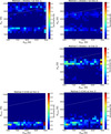 |
Fig. 5. Scatter plots of the 226 LFPs where SPINOR 2D returns B > 7 kG at log(τ) = 0 (BSP2). The y axis indicates magnetic field values obtained with each of the three alternative methods (direct Zeeman splitting and COG methods, BZ and BCOG respectively) as described in the text and displayed in Table 1. From top to bottom: Methods 1, 2, and 3 for line 1 at λ = 6301.5 Å (subscript 1, left plots) and for line 2 at λ = 6302.5 Å (subscript 2, right plots). Dashed lines represent expectation values if both methods give identical results (white). |
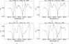 |
Fig. 6. Four examples of observed Stokes V profiles in the LFPs. The vertical lines indicate the position of the λ− (blue) and λ+ (red) used to calculate the magnetic field strength with Method 1. The headers of the plots indicate the magnetic field strengths as derived from: SPINOR 2D inversions (BSP2), Method 1 applied to the Fe I line at λ = 6301.5 Å (BZ1), and Method 1 applied to the Fe I line at λ = 6302.5 Å (BZ2). |
In contrast, Method 2 (middle panel in Fig. 5) finds a field strength distribution centered at ∼7 kG; whilst Method 3 (bottom panels) mainly senses field strengths of the order of 2.5 kG for line 1 and around 3 kG for line 2.
The correlation between the field strengths from the methods and the results from SPINOR 2D are very low, particularly for Method 3. However, there is some level of correlation between SPINOR 2D and the cloud of pixels displaying the strongest field solution in Method 1. Likewise, there is a good correlation between the clouds of pixels displaying the weaker field solution in Method 1 with the solutions in Method 3.
The large discrepancy between the methods has to do with the fact that only the LFPs have been plotted. Ideally, to check if the methods are consistent at lower field values but depart from each other only at strong fields, scatter-plots with a larger sample of pixels covering a broader range of magnetic field values in the x axis are needed. However, it is not possible to apply the direct Zeeman splitting method to profiles that do not show distinguishable sigma components, that is, to most of the penumbral pixels, except for the LFPs.
For the COG method, differences are expected due to velocity gradients, vertical field gradients, temperature, and so on that are not taken into account by the method (the gradients in B and vLOS are not taken into account in Eqs. (1) and (2)). The presence of such gradients is indicated by the asymmetries of the Stokes profiles. Moreover, if there are spatially unresolved areas containing field inhomogeneities (e.g., different field strengths and/or different field polarities located next to each other within the same resolution element), then the resultant line profiles from such pixels will be the summation of all the different magnetic components, meaning that the number of lobes in the observed Stokes V profiles will depend on the number of unresolved components (e.g., Stenflo 1993). Most Stokes V profiles from the 226 LFPs display more than two lobes, suggesting the presence of different magnetic field components in each of those pixels. Nonetheless, according to Methods 1 and 2, the very large wavelength separation between the most external lobes observed in the Stokes V profiles could still reflect that one of the field components is particularly strong. In such a scenario, an important aspect to consider is if the Paschen-Back effect would play an important role under the presence of such strong fields, that is, if the splitting of atomic levels caused by such strong external magnetic fields would dominate over the LS coupling.
The Paschen-Back regime occurs when ΔEik ≫ μBgLMB, where ΔEik is the energy difference in the atom between the terms of the multiplet structure, μB is the Bohr magneton, gL is the Landé factor, M is the magnetic quantum number, and B is the magnetic field strength. The Fe I 5P2−5D2λ = 6301.5 Å and the Fe I 5P1−5D0λ = 6302.5 Å lines belong to the same multiplet No. 816 (Moore 1945). The minimum energy difference of the lower levels of these lines is ΔEik ≈ 0.032 eV and leads to a magnetic field “threshold value” for the Paschen-Back effect of the order of 103 kG, a value that is well above the field strength values inferred by Methods 1, 2, and the SPINOR 2D inversions. Nonetheless, according to laboratory experiments, the Paschen-Back effect actually takes place under the presence of magnetic fields with strengths of 10 − 100 kG when the multiplet splitting energy difference is so small that the two adjacent lines of the same multiplet are separated by a distance of less than 1 Å (Frisch 1963). In the present case, since the analyzed pair of Fe I lines are separated by around 1 Å and the Zeeman splittings being discussed are seemingly very large (corresponding to field strengths approaching 10 kG in some LFPs according to Method 1), it is possible that the Paschen-Back effect begins to play some role in the magnetic splitting for those cases. However, even within the Paschen-Back regime, the magnetic field could still be measured with sufficient accuracy according to the laboratory results of Moore (1945).
Another plausible scenario is that the observed multi-lobed Stokes V profiles are produced by two unresolved atmospheric components that display large differences in their Doppler velocity (e.g., Solanki & Montavon 1993; Martínez Pillet 2000; Borrero & Bellot Rubio 2002; Schlichenmaier & Collados 2002; Bellot Rubio et al. 2004). One of the components could be associated with the umbral magnetic field in the sunspot (i.e., nearly at rest) and the second one with the filamentary CEF penumbra (strongly redshifted). This possibility is considered in the following section based on the fact that all the LFPs appear to be mostly located near, or at the umbral/penumbral edge (see Figs. 2a and 3a).
5. Inversions
In order to gain more insight into the reliability of the large magnetic field strengths returned by the SPINOR 2D inversion code, we now apply five additional inversions, considering two atmospheric components in some of them. It is noteworthy that the inclusion of a second atmospheric component causes the number of free parameters, n, to increase to almost twice that in a single component model used in the SPINOR 2D inversions. While this can and should lead to a much better fit for a complex Stokes profile (lower χ2), it also increases the risk of obtaining artificial (unphysical) results.
The merit functions, χ2, are not computed in the same way by the different inversion codes; and hence, they are in principle not comparable among each other. To perform a valid comparison between the different fits, in the following, the minimum χ2 is chosen to be the sum over the squared differences between the observed and the synthetic profiles resulting from the best fits in each case.
In Tables 2 and 3, we show some of the parameters corresponding to the best fits of the Stokes profiles in the two selected LFPs obtained from all six different inversions. These inversions can be classified into two categories, as follows.
Parameters resulting from four different height-dependent inversions which were applied to the two sets of observed Stokes profiles ((a) and (b)) and to their corresponding deconvolved Stokes profiles ((c) and (d)) from the two selected LFPs.
Parameters resulting from two height-independent inversions: (e) two-components Milne-Eddington inversions applied to the two sets of observed Stokes profiles (black dashed lines in Fig. 7) and, (f) two-components SPINOR 1D inversions applied to the corresponding deconvolved Stokes profiles (black dashed lines in Fig. 8) of the two selected LFPs (blue markers on Fig. 3a).
5.1. Height-dependent inversions
The first category includes height-dependent inversions (Table 2), that is, inversions in which all the parameters are allowed to vary with optical depth (with nodes being set at log(τ) = − 2.0, −0.8 and 0), such as (a) SPINOR 2D inversions with 18 free parameters; (b) SPINOR 1D (Frutiger et al. 2000) two-component inversions applied to the observed Stokes profiles (best fits are shown by green curves in Fig. 7), with 37 free parameters; (c) SPINOR 1D single component applied to the deconvolved Stokes profiles, with 18 free parameters and (d) SPINOR 1D two-component inversions applied to the deconvolved Stokes profiles, with 37 free parameters.
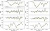 |
Fig. 7. Observed Stokes profiles (dashed curves), and their best fits returned by SPINOR 2D (orange curves), SPINOR 1D two-component height-dependent inversions (green curves) and Milne-Eddington two-component inversion (purple curves) in the two selected LFPs. Plots are in the same format as plots in Fig. 4. |
Inversions (c) and (d) are intended to resemble the SPINOR 2D technique as far as accounting for the instrumental effects over the observed Stokes profiles is concerned, although the treatment is not as consistent as that by SPINOR 2D. We retrieve the deconvolved Stokes profiles from the spatially degraded observed Stokes profiles by using an effective point spread function (PSF; Danilovic et al. 2008) constructed from the pupil function of the 50 cm Hinode SOT (Suematsu et al. 2008) and applying the Richardson-Lucy deconvolution method (see Richardson 1972 and Lucy 1974 for details). The resultant deconvolved Stokes profiles in the selected pixels are displayed in Fig. 8 (black dashed curves) together with their best fits obtained by SPINOR 1D (c) and (d) (orange and green curves in Fig. 8, respectively).
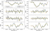 |
Fig. 8. Deconvolved Stokes profiles (dashed curve) and their best fits returned by SPINOR 1D inversions, using a single-component height-dependent model atmosphere (orange curves), a two-component height-dependent model (green), and a two-component height independent model atmosphere (purple curves) for the two selected LFPs. Plots are in the same format as plots in Fig. 4. |
5.2. Height-independent inversions
The second category corresponds to height-independent inversions (Table 3), that is, we assume no variation with optical depth of atmospheric parameters by using (e) a two-components Milne-Eddington inversion (Skumanich & Lites 1987; Lagg et al. 2004, 2009; Borrero et al. 2011) applied to the observed Stokes profiles (best fits are shown by purple curves in Fig. 7), with 15 free parameters; and (f) two-component one-node SPINOR 1D inversions applied to the deconvolved Stokes profiles (best fits are shown by purple curves in Fig. 8), with 17 free parameters.
6. Results
The SPINOR 2D best-fits give B ∼ 8.3 kG at log(τ) = 0 for the profiles in pixel 1, while B = 8 kG is obtained for both pixels at log(τ) = − 0.8 (see Table 2), with χ2 = 14 and 35 for each fit, respectively. These fits do not succeed in perfectly reproducing the reversed central lobes of the Stokes V profiles observed in both pixels. The deconvolved spectra displayed in Fig. 8 also show the reversed central lobes in Stokes V, which suggests that they are not a result of the mixing of signals due to instrumental effects. Nonetheless, inversions (c) also fail to reproduce the central reversed lobes, providing a much poorer fit than SPINOR 2D (χ2 = 44 and 47 for each pixel, respectively, when taking into account an increased noise of ∼5σ in the deconvolved Stokes profiles caused by the deconvolution itself) and featuring B ∼ 7 kG at log(τ) = 0 in both pixels. Thus, in both cases, the one-component inversions cannot fit these four-lobe profiles to high precision. At the same time, both inversions return very large field values. Such extreme field values are likely the result of providing a good fit mainly to the external lobes of Stokes V to reproduce the large wavelength separation in terms of the Zeeman splitting.
While the height-dependent two-component inversions produce better fits to the four-lobe profiles than the one-component inversions, χ2 = 8 and 12 for each pixel respectively in inversions (b), and χ2 = 14 and 18 respectively in inversions (d), they also use a much larger number of free parameters than the one-component inversions, meaning that a comparison is not straightforward. Component 1 in inversions (b) and (d) gives B ∼ 4 − 4.2 kG and vLOS ∼ 1 km s−1 at log(τ) = 0 in both pixels, roughly consistent with the umbral environment in the vicinity of those pixels (B ∼ 4.2 kG at log(τ) = 0, according to SPINOR 2D). Furthermore, the vLOS in component 1 is relatively small in both pixels and at all three atmospheric layers, as expected for umbral environments. In contrast, component 2 in inversions (b) and (d) gives B ∼ 4.4 and ∼4.9 kG, respectively, for pixel 1 at log(τ) = 0; and B ∼ 5 and 5.8 kG, respectively, for pixel 2; with vLOS ≳ 16 km s−1 and with the filling factors α, that is, the mixing ratio between component 1 and 2, being slightly larger for component 2 than for component 1 in both pixels. Component 2 in both pixels could then correspond to the tails of the penumbral filaments harboring the CEF, with a large redshift and stronger fields than in the surrounding umbra; which is qualitatively compatible with the results from SPINOR 2D, but quantitatively suggests lower penumbral field strengths of the order of 4 − 5 kG (although approaching 6 kG in one pixel).
The SPINOR 1D inversion code can find a solution involving two components, one of which is strongly wavelength shifted to mimic the seemingly very strongly split spectral line. This nearly halves the field strength, although even in this case we get B values reaching up to nearly 6 kG. These are still very large field strengths and are atypical for penumbral environments; they are close to the record measurement of 6.1 kG in sunspot umbrae (Livingston et al. 2006). However, due to the large number of free parameters involved, it is difficult to judge if the results they provide are more reliable than those from SPINOR 2D inversions.
A formal approach to compare the different results obtained from inversions that consider different model assumptions would be through the comparison of their error bars. Unfortunately, specifying the uncertainties in the fitted atmospheric parameters that take into account the possible degeneracies between parameters is an intrinsic difficulty facing inversions. Especially in the case of the spatially coupled inversions, the changes in the parameters of a single pixel severely affect the result – and therefore the uncertainties of the parameters – in the neighboring pixels. This fact makes the computation of formal errors for a single pixel impossible, and therefore the SPINOR 2D inversion code does not provide errors.
As a simple proxy for the quality of the fits, we compare the models using the Bayesian information criterion (BIC; Schwarz 1978), which is based on the crude approximation of Gaussianity of the posterior with respect to the model parameters:
 (3)
(3)
where  is the merit function of the best fits to the Stokes profiles in each model, n is the number of free parameters, and N is the number of observed points. The computed values of the BIC for each fit are shown in Tables 2 and 3. The model with the smallest value of the BIC is the preferred one. The height-dependent model preferred by the BIC is SPINOR 2D in both pixels. However, one of the fundamental problems of this criterion is that it penalizes all parameters equally, not taking into account situations in which data do not constrain some parameters (see e.g., Asensio Ramos et al. 2012).
The height-independent two-component inversions (e) and (f) give nearly identical results to each other in both pixels, with lower field strengths of around 3.5 kG in component 1, which is almost at rest (vLOS < 1 km s−1) compared to component 2 in which B ∼ 4 kG and vLOS ∼ 16 km s−1. However, the resultant values of B and vLOS given by the two height-independent inversions (e) and (f) generally resemble the results from the height-dependent two-component inversions (b) and (d) at log(τ) = − 0.8. This is not surprising because the sensitivity to vLOS and B perturbations is higher at log(τ) = − 0.8 than at log(τ) = 0 for the Fe I 6302.5 Å line (see, e.g., response functions computed by Cabrera Solana et al. 2005 and Fig. 1). Even if the absorption line is not formed at a single depth, the height-independent inversions mainly provide information on the physical conditions prevailing at depths at which the line is more sensitive. Therefore, if stronger magnetic fields are present in deeper layers of the solar atmosphere (e.g., at log(τ) = 0), as suggested by the results of inversions (a), (b), (c), and (d), they cannot be retrieved by inverting the Stokes profiles of the current wavelength range with a height-independent inversion technique only.
The BIC values obtained for inversions (e) and (f) are only slightly better than the ones obtained for SPINOR 2D in both pixels. Even if they both succeed in capturing many relevant aspects of all four Stokes profiles (despite the increased noise in the deconvolved spectra), it is very unlikely that the physical parameters in the pixels of interest display no gradients with height. Generally in sunspots, one would rather expect large gradients of the physical parameters with height (particularly of the magnetic field) as supported by MHD simulations. In such cases, height-dependent inversions provide a more appropriate model atmosphere. The SPINOR 2D inversions are the most reliable model in this sense, since they take into account the height stratification of the physical parameters while keeping a good balance between the quality of the fit and the number of free parameters in the model, according to the obtained BIC values in the two studied pixels with peculiar spectra.
7. Strong photospheric penumbral fields in a MURaM MHD simulation
We now use the 3D high-resolution sunspot simulation by Rempel (2015), see also Siu-Tapia et al. (2018), with a pixel resolution of 48 km in the horizontal direction and 24 km in the vertical direction to investigate the possible origin of super-strong penumbral magnetic fields associated with supersonic downflows in CEF-carrying filaments, and to compare their synthetic spectra with the observed Stokes profiles reported in the previous sections.
As reported by Rempel (2015) and Siu-Tapia et al. (2018), the sunspot simulation covers a time-span of 100 solar hours and after t ∼ 50 h, it displays radially aligned penumbral filaments with fast Evershed ouflows along them; in some regions of the penumbra however, the filaments carry instead a CEF, that is, radial inflows directed toward the sunspot umbra and strong downflows (vz < −8 km s−1) at the end of such filaments, in their inner endpoints where the magnetic field is noticeably enhanced, up to values of around 5 kG and γ ∼ 40° near the local τ = 1 level (see for example Fig. 9, cf. Fig. 2 in Siu-Tapia et al. (2018)).
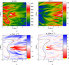 |
Fig. 9. Portion of the inner penumbra in the MURaM sunspot simulation by Rempel (2015) with some filaments hosting a counter-EF (see also Siu-Tapia et al. 2018). The maps show: panel a: magnetic field strength B [G]; panel b: field inclination with respect to the vertical γ [°], i.e., γ = 0° represents a vertical field of umbral polarity, γ = 90° a horizontal field, and γ = 180° a vertical field of opposite polarity to the umbra; panel c: radial flow velocity vr [km s−1]; and panel d: vertical flow velocity vz [km s−1]. Negative vr and vz values (red-to-yellow colors) indicate inflows and downflows, respectively. This sign convention differs from the one used in observational studies, where negative values denote flows moving towards the observer along the LOS. The black contour lines were placed at Ic/IQS < 0.45 near the umbra(left)-penumbra(right) boundary. All maps show the corresponding physical parameters at log(τ) = 0. |
In a relatively quick and simple attempt to quantify the effect of the 3D atmospheric structure and magnetic field on the profiles of the analyzed spectral lines, we employed the forward part of the SPINOR code (STOPRO) to solve the radiative transfer equation in the MURaM cube analyzed by Siu-Tapia et al. (2018), which was obtained with nongray radiative transfer. Figure 10a shows the emergent synthetic spectra from a vertical column located close to the inner edge of the simulated penumbra and which, at the log(τ) = 0 level, intersects with the tail of a CEF-carrying filament and contains supersonic downflows at that height. Similarly to the observed Stokes profiles for the pair of Fe I lines from the LFP in AR 10930, the synthetic Stokes profiles from the MHD simulations are highly asymmetric, display large redshifts, and show multi-lobed Stokes V profiles.
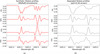 |
Fig. 10. Panel a: set of emergent synthetic Stokes profiles in the MURaM sunspot simulation at the location of a supersonic downflow in the tail of a CEF-carrying filament. The spectra were synthesized using the SPINOR code (STOPRO routines). Panel b: degraded Stokes profiles obtained from the convolution of the synthetic spectra with a PSF of 0.16 arcsec, similar to the case of the Hinode telescope. |
In Fig. 10b, we display degraded Stokes profiles which were obtained by convolving the synthetic spectra in Fig. 10a with an effective PSF=0.16″ (Danilovic et al. 2008) constructed from the pupil function of the 50 cm Hinode SOT (Suematsu et al. 2008). The degraded profiles also show the main characteristics described above and resemble the observed Stokes profiles presented in the previous sections, which are even more extreme.
Such complex shapes in the MHD case are mainly the result of the large vertical gradients in all the atmospheric quantities and the magnetic field structure. In particular, the stratification of the field strength (Fig. 11a), the flow velocity (Fig. 11b), and field inclination (Fig. 11c), qualitatively resemble the SPINOR 2D results in the LFPs (cf. Table 2), that is, while the field strength and downflow speeds increase with depth, the field inclination increases with height. Another important aspect that might contribute to the complexity of the emergent spectra is the presence of a shock which is seen as the sudden transition of the downflow speed from subsonic to supersonic near log(τ) = − 1, and as the sudden variation of all the physical parameters shown in Fig. 11.
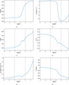 |
Fig. 11. Vertical profiles, in a log(τ)-scale, of the MHD physical parameters leading to the emergent synthetic Stokes profiles shown in Fig. 10, at the location of a supersonic downflow in the tail of a CEF-carrying filament: panel a: magnetic field strength, panel b: vertical flow velocity (negative values indicate downflows), panel c: temperature, panel d: field inclination, panel e: gas density, and panel f: geometrical height at the location of the grid-cell containing the supersonic downflows from the MURaM simulation. Vertical dashed lines delimit the approximate τ−range where the lines show a significant response, i.e., between log(τ) = − 2 and 0. |
The presence of strong magnetic fields at the local log(τ) = 0 level (in excess of 5 kG) in the simulations is mainly due to the influence of the neighboring umbral field and the highly depressed surfaces of constant optical depth as reported by Siu-Tapia et al. (2018). Such surface depression is of the order of 400 − 600 km in the analyzed case (see Fig. 11f), and is related to a strong decrease of the gas density beneath log(τ) = − 1 (see Fig. 11e).
Thus, given the similarity of the physical scenarios that the observations and the simulations present, the determination of the physical processes involved in the maintenance and amplification of the field in the simulations can provide insight into the possible origin of super-strong photospheric magnetic fields observed in sunspot penumbrae.
7.1. Induction equation
In order to study how the vertical field is maintained in the penumbra, we evaluate the different terms of the induction equation in the simulation box:
 (4)
(4)
We analyze the different terms in Eq. (4) during the time-period from 60 to 70 solar hours (the range of time during which the counter-EF are found in the simulations) of the total of 100 h simulations run (see Siu-Tapia et al. 2018 for details), using the transformation to cylindrical coordinates to separate the direction along and perpendicular to the penumbral filaments, that is., r, θ, and z coordinates; and by separating outflows (vr > 0) from inflows (vr < 0), and upflows (vz > 0) from downflows (vz < 0) in the simulated penumbra.
As reported by Siu-Tapia et al. (2018), the vertical field component is noticeably enhanced at the tails of the penumbral filaments, that is, at the filament end-points hosting sinks in both filaments carrying a normal-EF (NEF, i.e., outflows) and those carrying a counter-EF (CEF, i.e., inflows), which are mainly located close to the outer and inner penumbral boundary, respectively (see e.g. Fig. 3 in Siu-Tapia et al. 2018). Therefore, we explore the mechanisms that can lead to the amplification of the magnetic field strength at those places. We use different masks in order to separate the sinks (downflows) that occur at the tails of the NEF-carrying filaments (regions where vz < 0 and vr > 0 in the outer penumbra) from those sinks that happen at the tails of the CEF-carrying filaments (regions where vz < 0 and vr < 0 in the inner penumbra).
Figure 12 displays the contributions of each term in Eq. 4 to the vertical field component, horizontally averaged over the sinks of the NEF (left plot) and over the sinks of the CEF (right plot), and focusing the averages on localized regions that have fairly strong fields (Bz < −2 kG for the sinks of the NEF and Bz > 2 kG for the sinks of the CEF) as well as supersonic downflows at log(τ) = 0. In both cases, NEF and CEF sinks, the contributions from stretching, advection, and divergence are mostly in balance, implying that the residual terms, which have potential contributions from the numerical magnetic diffusivity and from time variations (green lines), do not play a significant role in shaping the magnetic structure of the penumbra in these simulations during the analyzed time period.
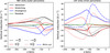 |
Fig. 12. Average contributions to the induction equation from advection (solid black), field-line stretching (solid red), flow divergence (solid blue), and a residual term (solid green) to the vertical field component at the sinks of the NEF (left) and at the sinks of the CEF (right). The averages have been focused on localized regions that have fairly strong fields (Bz < −2 kG for the sinks of the NEF and Bz > 2 kG for the sinks of the CEF) and supersonic downflows at the local log(τ) = 0 level. The residual term represents the numerical magnetic diffusivity as an approximated magnitude that is calculated by the negative sum of the advective, stretching, and divergent terms; but it also contains potential contributions from time variation. The dashed and dotted lines represent approximated terms that provide a major contribution to the advective term (black) and to the stretching term (red), whose general expressions are indicated in the lower labels. The dash-dotted blue line represents the contribution to the divergence term due to flows perpendicular to the vertical field component, i.e., radial and azimuthal flow components. |
The roles of advection and divergence in the vertical induction (black and blue solid lines, respectively) are opposed to each other in both penumbral regions. In addition, they appear with a sign swap in the outer penumbra (left panel) compared to the inner penumbra (right panel). However, the roles of advection and divergence for maintaining the vertical field component are the same in both regions given that Bz < 0 at the sinks of the NEF and Bz > 0 at the sinks of the CEF, which causes the sign swap in the vertical induction.
Thus, at the sinks of the NEF (outer penumbra, left plot), there is an opposed contribution from the advective term to the maintenance of the (negative) vertical field component at all heights of the analyzed z-range (where z = 0 corresponds to the average height of the log(τ) = 0 surface in the quiet sun). In contrast, the stretching term behaves as a source for the (negative) vertical field component in the outer penumbra, above z ∼ −200 km. The major contribution to this term comes from vertical stretching (red dotted line), that is,  due to a strong downward transition of the downflow speeds (from subsonic to supersonic) that leads to the steepening of
  near z ∼ −200 km (generally, the supersonic NEF sinks are shallower than in the CEF case; for an example see the white contours in the vz panel of Fig. 3 in Siu-Tapia et al. (2018) which enclose regions where vz < −8 km s−1). Deeper down, below z ∼ −200 km, there is a radial shear profile (red dashed line) due to a radial outward increase of the downflow speeds,
  , that also contributes to the maintenance of the (negative) vertical field component in the outer penumbra. However, the major source comes from the divergence term (blue line) due to the converging aspect of the downflows, namely ∇ ⋅ v < 0. The dominant contribution to this term in the near-surface layers is given by flows that are perpendicular to the vertical field component, vr and vθ, that is, by a horizontal convergence of the downflowing material (dash-dotted blue line). The remainder is due to the term
  , which becomes negative below z ∼ −200 km.
Similarly, advection plays an opposite role for the maintenance of the (positive) vertical field component at the sinks of the CEF in the inner penumbra (right plot in Fig. 12). However, the role of stretching is not significant above z ∼ −400 km in this case (i.e., the height at which most of the CEF sinks become supersonic; see example in Figs. 11b and f). Notwithstanding, due to the strong downward acceleration of the gas at the sinks of the CEF, vertical stretching acts as a source for the (positive) vertical field above z ∼ −400 km, i.e.,  . Likewise, a radial inward increase of the downflow speed at the sinks of the CEF leads to a radial shear term that contributes positively below z ∼ −400 km, namely
  . The dominant positive contribution to the (positive) vertical field component is given by the divergence term (i.e., ∇ ⋅ v < 0, because Bz is positive in the inner penumbra), which means that similarly to the NEF sinks the CEF sinks are also convergent downflows, which implies compression and amplification of the magnetic field.
7.2. Force balance
In order to investigate how the strongest fields in the penumbra are balanced, we follow the analysis performed by Rempel (2011) and Siu-Tapia et al. (2018) and use the following force balance equation which is derived from the momentum equation by assuming stationarity:
 (5)
(5)
Each term in the above equation is then separated into a radial and a vertical component; and a residual force term is introduced as the negative sum of the pressure, the acceleration, and the Lorentz force contributions in the corresponding direction given that the viscosity force terms are not explicitly calculated.
Figure 13 shows the average radial and vertical force balance at the strong field regions of the inner penumbra with supersonic downflows of the CEFs. In both directions the forces are mostly in balance and the residual forces are almost zero. These plots show that acceleration forces (blue lines) are very significant in the radial direction but are almost negligible in the vertical direction, which means that the system is close to magneto-hydrostatic in the vertical direction given that the Lorentz force (red line) nearly completely balances with the pressure forces (black line).
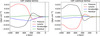 |
Fig. 13. Force balance in the radial (left) and vertical (right) directions. The force terms have been horizontally and temporally averaged over the places with strongest fields and supersonic downflows of the CEF in the inner penumbra. Black: pressure forces, red: Lorentz forces, blue: acceleration forces, green: residual forces. The vertical gray dashed lines are placed at the average height of the log(τ) = 0 level in the selected regions and are located nearly 400 km beneath the average height of the log(τ) = 0 surface in the quiet sun (i.e., z = 0 km, black dashed line). |
The average height of the log(τ) = 0 level over the selected regions lies almost 400 km below its average height in the quiet sun. Such average height is considerably deeper than in the whole penumbra (approximately at z = −200 km) and even deeper than in the inner penumbra (z ∼ −250 km).
Figure 14 displays the Lorentz force separately for the magnetic pressure term (−∇[B2/8π], red lines) and the magnetic tension term ([B ⋅ ∇]B/4π, magenta lines) in the radial (solid) and vertical (dashed) directions, which have been averaged over the strong field regions of the inner penumbra with supersonic downflows (same mask as in Fig. 13). Looking at the individual components of the Lorentz force, we see in the vertical direction that the strongest fields in the simulation are less force-free in the deeper domain, where the gas pressure (black dashed line) is strong enough to balance, but they become mostly force-free near the observable photosphere and in the layers above. In contrast, in the radial direction, the magnetic pressure force dominates over the magnetic tension force at most heights. However, the gas pressure force term (black solid line) is also large enough in the radial direction to considerably contribute to keep the balance. In addition, we have seen that the contribution of the radial acceleration forces (blue line in Fig. 13) plays an important role for maintaining the force balance in the radial direction.
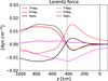 |
Fig. 14. Radial (solid) and vertical (dashed) Lorentz force terms separated for the magnetic pressure (red) and the magnetic tension (magenta) forces at the places with strongest fields and supersonic downflows of the CEF in the inner penumbra. The radial (black solid) and vertical (black dashed) gas pressure forces are overplotted for comparison. The same format is used as in Fig. 13. |
8. Discussion and conclusion
Inversion techniques are currently the most powerful tools to infer the physical properties of the solar atmosphere from polarization line profiles, being able to provide reliable and robust results from many types of Stokes profiles according to numerical tests (e.g., Ruiz Cobo 2007). There are several different inversion techniques in the literature, each of them with its own advantages and shortcomings, which largely depend on the addressed problem. Certainly, after any Stokes inversion the results need always to be validated and one needs to be aware that the resulting model atmosphere is not necessarily the real one since the solution might not be unique or the model underlying the inversion not appropriate to the actual solar situation. Nonetheless, as stated by Sabatier (2000), by means of Stokes inversions, it is generally possible to retrieve as much information as possible for a model which is proposed to represent the system in the real world.
The existence of B > 7 kG in the inner penumbra of a sunspot would require an unusually deep Wilson depression to be consistent with idealized magnetohydrostatic models of sunspots (Livingston et al. 2006). However, besides the non-negligible dynamical effects of the studied penumbra, the magnetic field does not have to be in a maximally non-force-free state as usually assumed for the photosphere. We find that in the MHD simulations, the strongest fields in the penumbra (∼5 kG) are vertically close to force-free in the observable photosphere and the gas pressure is sufficient to reach a force balance in the deeper layers. Although these fields are less force-free in the radial direction, the radial gas pressure force provides a sufficient balance to keep the system in near equilibrium, but it is only with the contribution of radial acceleration forces that an almost complete balance can be reached. In this sense, the existence of 7 kG magnetic fields in the photosphere would be possible in a highly dynamical environment, such as that inferred by the SPINOR 2D inversions, that is, with supersonic counter-Evershed flows sinking supersonically in the inner penumbra. Such superstrong field concentrations would likely fan out significantly with height and remain close to potential in the observable photosphere.
Field strengths larger than 7 kG in penumbral environments have previously been reported by van Noort et al. (2013). These latter authors obtain similarly large field strengths in supersonic downflow regions in the peripheral penumbra of a sunspot; and they too use SPINOR 2D inversions. Nonetheless, they observe B > 7 kG only in the deepest layer (log(τ) = 0) and obtain good agreement between the inversion results and a MURaM simulation of a sunspot by Rempel (2012). van Noort et al. (2013) propose a scenario in which the high magnetic field values are the result of a field intensification in the deep photosphere due to the interaction of the supersonic downflows with an external magnetic barrier (e.g., with a plage region). Such a scenario could also be valid for the present observations, with the umbral field playing the role of the magnetic barrier.
According to the SPINOR 2D results (e.g., Fig. 3b and Table 2), most of the magnetic fields whose strength is above 7 kG (LFPs) are nearly vertical and have the same polarity as the umbra, which is negative. In addition, they are associated to supersonic downflows, even exceeding vLOS = 20 km s−1 at log(τ) = 0 in some LFPs. Moreover, the regions in the sunspot where B > 5 kG are also associated with supersonic LOS flow velocities (see, e.g., Fig. 5a in Siu-Tapia et al. 2017). As displayed in Fig. 3a, the LFPs with B > 7 kG (yellow pixels) are surrounded by those weaker fields, which are still in excess of 5 kG (red pixels), in a supersonic flow environment (see also Fig. 2). A very low density of the supersonic downflowing material could also explain the observation of unusually strong magnetic fields in the penumbra, since it would cause the optical depth layers to be strongly depressed. In addition, their close vicinity to the umbral field also plays a role.
This is in agreement with MHD simulations of counter-Evershed flows (Siu-Tapia et al. 2018, and Sect. 7), which show a ∼400 km depressed τ = 1 surface on average (and up to 600 km, with respect to its average height in the quiet sun) at the tails of the CEF-carrying filaments, where the supersonic downflowing material becomes a very low density gas (see also Fig. 11e). As a consequence, deep-lying field strengths of the order of 5 kG in the inner penumbra (near the umbra) are visible at the τ = 1 level in those simulations.
The resultant synthetic Stokes profiles associated to photospheric fields of the order of 5 kG and downflow speeds of 10 − 12 km s−1 in the simulated penumbra display large asymmetries, redshifts, and multiple lobes in their Stokes V profiles, in agreement with the observed spectra in the LFPs. This result supports the possibility that the observed Stokes profiles associated with the LFPs in AR10930, which display even more extreme characteristics, are produced by larger fields and stronger downflows as inferred by the SPINOR 2D inversions (Fig. 3b).
The strong penumbral magnetic fields in the simulations (nearly 5 kG at the local τ = 1 level) are mainly due to the influence of the neighboring umbral field, the highly depressed surfaces of constant optical depth, and the formation of shocks by the transition of the downflow speeds from subsonic to supersonic; but there is also a local intensification of the field that can be associated to the converging aspect of the supersonic downflows, which lead to a compression and intensification of the vertical magnetic field component in the inner penumbra.
A similar mechanism amplifies the negative vertical field component at the sinks of the NEF in the outer penumbra in the simulations, where the field bends over and the downflows are convergent. There, the negative vertical field component can additionally be intensified by vertical stretching due to the strong downward acceleration of the gas up to supersonic speeds. These results are in agreement with the proposed scenario by van Noort et al. (2013) to explain the possible observation of superstrong fields associated with peripheral downflows in the penumbra of the leading spot of NOAA AR 10933.
According to the BIC (Schwarz 1978), which assesses a best fit based on the balance between the quality of the fit and the number of free parameters considered by the model, the preferred height-dependent model atmospheres for the LFPs are those provided by the SPINOR 2D inversions. Furthermore, given the extreme characteristics of the observed Stokes profiles associated with the sinks of the CEF in the LFPs and their resemblance to the synthetic spectra derived from the MHD simulations, we finally cannot easily discard the possibility that we are dealing with actual observations of B ∼ 7 kG and even larger in regions of supersonic downflowing material (up to vLOS ∼ 35 km s−1) with very low densities, where similar mechanisms to those occurring in the analyzed simulations might explain their origin.
The major strength of SPINOR 2D lies in its simultaneous coupled inversion of all the pixels to self-consistently take into account the influence of stray light from neighboring pixels. This approach is able to reproduce complex multi-lobed profiles with a simple one-component atmosphere per pixel, thus maintaining an acceptable number of free parameters, which significantly enhance the reliability and the robustness of the inversion results. However, we have seen that the highly complex observed Stokes profiles cannot be perfectly reproduced with any of the presented inversion techniques without almost doubling the number of free parameters. The inherent complexity of these profiles may involve physical aspects that are not considered within the assumptions and approximations made by the inversion codes, which could lead to significant errors in the returned values. These assumptions include hydrostatic equilibrium, which is unlikely to be satisfied in such a dynamic environment.
Finally, the field estimations performed by means of the Zeeman splitting and the COG method (Methods 1, 2, and 3) provide results that are not entirely consistent among one another. Unfortunately, all these methods are unable to take into account the errors from the instrumental effects. Moreover, Methods 1 and 2 are only reliable for ideal cases, such as when they are applied to single-component profiles produced by homogeneous magnetic fields, which is clearly not the case for the LFPs with highly asymmetric and multi-lobed Stokes profiles. As a consequence, the possibility of two (horizontally) unresolved structures with a large velocity difference cannot be ruled out either, in spite of the shortcomings of the two-component height-dependent and height-independent inversions. Unusually strong penumbral magnetic fields (5–6 kG) also show up as the most plausible physical solution in some of the two-component models. However, the existence of two Doppler-shifted components (one carrying nearly 15 km s−1 and the other with gas almost at rest) coexisting over several neighboring pixels would require an unresolved fine structure with subresolution canals of two types over an extended area. These extreme gradients in velocity required to be present in the one-resolution element to produce the observed spectra are considerably less plausible. A solution where the pixels are smoothly connected (as in the 2D inversions), with a height gradient within the line-forming region could represent a more plausible scenario and is in agreement with MHD simulations.
For future work, it would be interesting to investigate how the presence of superstrong magnetic fields in the photosphere affects the shape of the observed Stokes profiles in the pair of Fe I lines when considering the Paschen-Back effect. This will be useful to determine whether or not such effects need to be taken into account by the inversion codes when dealing with photospheric field strengths of the order of 7 kG or larger.
Acknowledgments
This work was partly carried out in the framework of the International Max Planck Research School (IMPRS) for Solar System Science at the Max Planck Institute for Solar System Research (MPS) supported by the Max Planck Society. It was also supported by the Spanish Science Ministry “Centro de Excelencia Severo Ochoa” Program under grant SEV-2017-0709 and project RTI2018-096886-B-C51. The National Center for Atmospheric Research is sponsored by the National Science Foundation. Hinode is a Japanese mission developed and launched by ISAS/JAXA, with NAOJ as a domestic partner and NASA and STFC (UK) as international partners. It is operated by these agencies in co-operation with ESA and NSC (Norway).
References
- Asensio Ramos, A., Manso Sainz, R., Martínez González, M. J., et al. 2012, ApJ, 748, 83 [NASA ADS] [CrossRef] [Google Scholar]
- Bellot Rubio, L. R., Balthasar, H., & Collados, M. 2004, A&A, 427, 319 [NASA ADS] [CrossRef] [EDP Sciences] [Google Scholar]
- Borrero, J. M., & Bellot Rubio, L. R. 2002, A&A, 385, 1056 [NASA ADS] [CrossRef] [EDP Sciences] [Google Scholar]
- Borrero, J. M., Tomczyk, S., Kubo, M., et al. 2011, Sol. Phys., 273, 267 [Google Scholar]
- Cabrera Solana, D., Bellot Rubio, L. R., & del Toro Iniesta, J. C. 2005, A&A, 439, 687 [NASA ADS] [CrossRef] [EDP Sciences] [Google Scholar]
- Cauzzi, G., Smaldone, L. A., Balasubramaniam, K. S., & Keil, S. L. 1993, Sol. Phys., 146, 207 [NASA ADS] [CrossRef] [Google Scholar]
- Danilovic, S., Gandorfer, A., Lagg, A., et al. 2008, A&A, 484, L17 [NASA ADS] [CrossRef] [EDP Sciences] [Google Scholar]
- Evershed, J. 1909, MNRAS, 69, 454 [NASA ADS] [CrossRef] [Google Scholar]
- Frisch, I. E. 1963, Optical Spectra of Atoms (Moscow, Leningrad: Fizmatgiz) [Google Scholar]
- Frutiger, C. 2000, PhD Thesis, Institute of Astronomy, ETH Zürich, Switzerland [Google Scholar]
- Frutiger, C., Solanki, S. K., Fligge, M., & Bruls, J. H. M. J. 2000, A&A, 358, 1109 [NASA ADS] [Google Scholar]
- Georgoulis, M. K. 2005, ApJ, 629, L69 [NASA ADS] [CrossRef] [Google Scholar]
- Keppens, R., & Martínez Pillet, V. 1996, A&A, 316, 229 [Google Scholar]
- Lagg, A., Woch, J., Kripp, N., & Solanki, S. K. 2004, A&A, 414, 1109 [NASA ADS] [CrossRef] [EDP Sciences] [Google Scholar]
- Lagg, A., Ishikawa, R., Merenda, L., et al. 2009, ASP Conf. Ser., 415, 327 [NASA ADS] [Google Scholar]
- Lites, B. W., & Ichimoto, K. 2013, Sol. Phys., 283, 601 [NASA ADS] [CrossRef] [Google Scholar]
- Lites, B. W., Skumanich, A., & Scharmer, G. B. 1990, ApJ, 355, 329 [NASA ADS] [CrossRef] [Google Scholar]
- Lites, B. W., Elmore, D. F., & Streander, K. V. 2001, in Advanced Solar Polarimetry – Theory, Observation, and Instrumentation, ed. M. Sigwarth, ASP Conf. Proc., 236, 33 [NASA ADS] [Google Scholar]
- Lites, B. W., Akin, D. L., Card, G., et al. 2013, Sol. Phys., 283, 579 [NASA ADS] [CrossRef] [Google Scholar]
- Livingston, W. 2002, Sol. Phys., 207, 41 [NASA ADS] [CrossRef] [Google Scholar]
- Livingston, W., Harvey, J. W., Malanushenko, O. V., & Webster, L. 2006, Sol. Phys., 239, 41 [Google Scholar]
- Lucy, L. B. 1974, AJ, 79, 745 [NASA ADS] [CrossRef] [Google Scholar]
- Martínez Pillet, V. 2000, A&A, 361, 734 [NASA ADS] [Google Scholar]
- Mathew, S. K., Lagg, A., Solanki, S. K., et al. 2003, A&A, 410, 695 [NASA ADS] [CrossRef] [EDP Sciences] [Google Scholar]
- Mathew, S. K., Solanki, S. K., Lagg, A., et al. 2004, A&A, 422, 693 [NASA ADS] [CrossRef] [EDP Sciences] [Google Scholar]
- Moore, C. E. 1945, A Multiplet Table of Astrophysical Interest (Princeton: Princeton University Observatory) [Google Scholar]
- Okamoto, T. J., & Sakurai, T. 2018, ApJ, 852, L16 [Google Scholar]
- Rees, D. E., & Semel, M. D. 1979, A&A, 74, 1 [NASA ADS] [Google Scholar]
- Rempel, M. 2011, ApJ, 729, 5 [NASA ADS] [CrossRef] [Google Scholar]
- Rempel, M. 2012, ApJ, 62, 21 [Google Scholar]
- Rempel, M. 2015, ApJ, 814, 125 [NASA ADS] [CrossRef] [Google Scholar]
- Richardson, W. H. 1972, J. Opt. Soc. Am., 62, 55 [Google Scholar]
- Ruiz Cobo, B. 2007, in Modern Solar Facilities-Advanced Solar Science, eds. F. Kneer, K. G. Puschmann, & A. D. Wittmann, 287 [Google Scholar]
- Sabatier, P. C. 2000, J. Math. Phys., 41, 4082 [NASA ADS] [CrossRef] [Google Scholar]
- Schlichenmaier, R., & Collados, M. 2002, A&A, 381, 668 [NASA ADS] [CrossRef] [EDP Sciences] [Google Scholar]
- Schwarz, G. E. 1978, Ann. Stat., 6, 461 [NASA ADS] [CrossRef] [MathSciNet] [Google Scholar]
- Semel, M. 1967, Ann. d’Astrophys., 30, 513 [NASA ADS] [Google Scholar]
- Semel, M. 1970, A&A, 5, 330 [NASA ADS] [Google Scholar]
- Siu-Tapia, A. L., Lagg, A., Solanki, S. K., van Noort, M., & Jurčák, J. 2017, A&A, 607, A36 [NASA ADS] [CrossRef] [EDP Sciences] [Google Scholar]
- Siu-Tapia, A. L., Rempel, M., Lagg, A., & Solanki, S. K. 2018, ApJ, 852, 66 [NASA ADS] [CrossRef] [Google Scholar]
- Skumanich, A., & Lites, B. W. 1987, ApJ, 322, 473 [Google Scholar]
- Skumanich, A., Lites, B. W., & Martínez Pillet, V. 1994, Solar Surface Magnetism, 99 [Google Scholar]
- Solanki, S. K. 1987, PhD Thesis, Institute of Astronomy, ETH Zürich, Switzerland [Google Scholar]
- Solanki, S. K. 1993, Space Sci. Rev., 63, 1 [NASA ADS] [CrossRef] [Google Scholar]
- Solanki, S. K., & Montavon, C. A. P. 1993, A&A, 275, 283 [NASA ADS] [Google Scholar]
- Stenflo, J. O. 1993, Proc. Int. Conf. (Feidburg, Germany: Cambridge University Press), 301 [Google Scholar]
- Suematsu, Y., Tsuneta, S., Ichimoto, K., et al. 2008, Sol. Phys., 249, 197 [NASA ADS] [CrossRef] [Google Scholar]
- Tiwari, S. K., van Noort, M., Lagg, A., & Solanki, S. K. 2013, A&A, 557, A25 [NASA ADS] [CrossRef] [EDP Sciences] [Google Scholar]
- Tiwari, S. K., van Noort, M., Solanki, S. K., & Lagg, A. 2015, A&A, 583, A119 [NASA ADS] [CrossRef] [EDP Sciences] [Google Scholar]
- van Noort, M. 2012, A&A, 548, A5 [NASA ADS] [CrossRef] [EDP Sciences] [Google Scholar]
- van Noort, M., Lagg, A., Tiwari, S. K., & Solanki, S. K. 2013, A&A, 557, A24 [NASA ADS] [CrossRef] [EDP Sciences] [Google Scholar]
- Westendorp Plaza, C., del Toro Iniesta, J. C., Ruiz Cobo, B., & Martínez Pillet, V. 2001, ApJ, 547, 1148 [NASA ADS] [CrossRef] [Google Scholar]
All Tables
Results of direct measurement of Zeeman splitting (Methods 1 and 2) and COG method in two LFPs.
Parameters resulting from four different height-dependent inversions which were applied to the two sets of observed Stokes profiles ((a) and (b)) and to their corresponding deconvolved Stokes profiles ((c) and (d)) from the two selected LFPs.
Parameters resulting from two height-independent inversions: (e) two-components Milne-Eddington inversions applied to the two sets of observed Stokes profiles (black dashed lines in Fig. 7) and, (f) two-components SPINOR 1D inversions applied to the corresponding deconvolved Stokes profiles (black dashed lines in Fig. 8) of the two selected LFPs (blue markers on Fig. 3a).
All Figures
|
Fig. 1. Normalized response function of Stokes I (left) and Stokes V (right) to the magnetic field B, multiplied by 1/ΔτC[10−5 G−1], for the pair of Fe I absorption lines at 6301.5 and 6302.5 Å in the atmosphere inferred by the SPINOR 2D inversions for the penumbral pixel marked with a blue plus symbol in Fig. 3a. Some physical parameters for such an atmosphere are presented in Table 2. The horizontal dashed lines indicate the selected nodes for the SPINOR 2D inversion: log(τ) = 0, −0.8 and −2. |
| In the text | |
|
Fig. 2. Portion of the (center-side) penumbra of the main sunspot in AR 10930 (cf. Fig. 5 in Siu-Tapia et al. (2017)). Panel a: map of the magnetic field strength at log(τ) = 0, as inferred with SPINOR 2D inversions. The arrow points towards the solar-disk center. Panel b: line-of-sight velocity as inferred with SPINOR 2D inversions at log(τ) = 0. Positive values (red-to-yellow colors) indicate plasma motions away from the observer, while negative values (blue colors) indicate motions towards the observer. Solid and dashed black contour lines were placed at Ic/IQS = 0.26 and Ic/IQS = 0.94, respectively. The large penumbral sector where red-to-yellow colors dominate harbors a fast counter-EF which supersonically sinks (with speeds larger than 12 km s−1) near the inner penumbral boundary (Siu-Tapia et al. 2017). The color-bar scales have been saturated. |
| In the text | |
|
Fig. 3. Panel a: normalized continuum intensity map as observed by the Hinode SOT/SP in AR 10930. The red markers indicate the location of 845 pixels where the SPINOR 2D inversions return B ≥ 5 kG at log(τ) = 0, of which 226 harbor fields larger than 7 kG at log(τ) = 0 (yellow markers, also named in the text such as large-field-pixels or LFPs). The blue markers highlight the location of two LFPs (“+”: LFP 1, “×”: LFP 2) selected to test the robustness of our inversion solutions (see text). The arrow points towards the solar-disk center. Panel b: scatter plot of the magnetic field inclination in the local reference frame γLRF (after removal of the field azimuth ambiguity through the NPFC method) vs. the line-of-sight velocity vLOS, from SPINOR 2D at log(τ) = 0, for the 226 LFPs. |
| In the text | |
|
Fig. 4. Observed Stokes profiles (dashed curves) in two pixels (left: pixel 1, right: pixel 2) located at the inner penumbra of the CEF region (see blue crosses on maps displayed in Fig. 3a). From top to bottom: Stokes I, Q, U and V. The vertical lines in Stokes I and V panels indicate the position of the λ− (blue) and λ+ (red) used to calculate the magnetic field strength with three different methods (see the main text for a description of the methods): the solid lines in the Stokes V panels show the splitting derived from Method 1; the solid lines in the Stokes I panels correspond to the line splitting obtained with Method 2; and, the dashed lines in both I and V panels indicate the splitting derived from Method 3. The vertical dashed green line shows the wavelength position used to separate the two Fe I lines. |
| In the text | |
|
Fig. 5. Scatter plots of the 226 LFPs where SPINOR 2D returns B > 7 kG at log(τ) = 0 (BSP2). The y axis indicates magnetic field values obtained with each of the three alternative methods (direct Zeeman splitting and COG methods, BZ and BCOG respectively) as described in the text and displayed in Table 1. From top to bottom: Methods 1, 2, and 3 for line 1 at λ = 6301.5 Å (subscript 1, left plots) and for line 2 at λ = 6302.5 Å (subscript 2, right plots). Dashed lines represent expectation values if both methods give identical results (white). |
| In the text | |
|
Fig. 6. Four examples of observed Stokes V profiles in the LFPs. The vertical lines indicate the position of the λ− (blue) and λ+ (red) used to calculate the magnetic field strength with Method 1. The headers of the plots indicate the magnetic field strengths as derived from: SPINOR 2D inversions (BSP2), Method 1 applied to the Fe I line at λ = 6301.5 Å (BZ1), and Method 1 applied to the Fe I line at λ = 6302.5 Å (BZ2). |
| In the text | |
|
Fig. 7. Observed Stokes profiles (dashed curves), and their best fits returned by SPINOR 2D (orange curves), SPINOR 1D two-component height-dependent inversions (green curves) and Milne-Eddington two-component inversion (purple curves) in the two selected LFPs. Plots are in the same format as plots in Fig. 4. |
| In the text | |
|
Fig. 8. Deconvolved Stokes profiles (dashed curve) and their best fits returned by SPINOR 1D inversions, using a single-component height-dependent model atmosphere (orange curves), a two-component height-dependent model (green), and a two-component height independent model atmosphere (purple curves) for the two selected LFPs. Plots are in the same format as plots in Fig. 4. |
| In the text | |
|
Fig. 9. Portion of the inner penumbra in the MURaM sunspot simulation by Rempel (2015) with some filaments hosting a counter-EF (see also Siu-Tapia et al. 2018). The maps show: panel a: magnetic field strength B [G]; panel b: field inclination with respect to the vertical γ [°], i.e., γ = 0° represents a vertical field of umbral polarity, γ = 90° a horizontal field, and γ = 180° a vertical field of opposite polarity to the umbra; panel c: radial flow velocity vr [km s−1]; and panel d: vertical flow velocity vz [km s−1]. Negative vr and vz values (red-to-yellow colors) indicate inflows and downflows, respectively. This sign convention differs from the one used in observational studies, where negative values denote flows moving towards the observer along the LOS. The black contour lines were placed at Ic/IQS < 0.45 near the umbra(left)-penumbra(right) boundary. All maps show the corresponding physical parameters at log(τ) = 0. |
| In the text | |
|
Fig. 10. Panel a: set of emergent synthetic Stokes profiles in the MURaM sunspot simulation at the location of a supersonic downflow in the tail of a CEF-carrying filament. The spectra were synthesized using the SPINOR code (STOPRO routines). Panel b: degraded Stokes profiles obtained from the convolution of the synthetic spectra with a PSF of 0.16 arcsec, similar to the case of the Hinode telescope. |
| In the text | |
|
Fig. 11. Vertical profiles, in a log(τ)-scale, of the MHD physical parameters leading to the emergent synthetic Stokes profiles shown in Fig. 10, at the location of a supersonic downflow in the tail of a CEF-carrying filament: panel a: magnetic field strength, panel b: vertical flow velocity (negative values indicate downflows), panel c: temperature, panel d: field inclination, panel e: gas density, and panel f: geometrical height at the location of the grid-cell containing the supersonic downflows from the MURaM simulation. Vertical dashed lines delimit the approximate τ−range where the lines show a significant response, i.e., between log(τ) = − 2 and 0. |
| In the text | |
|
Fig. 12. Average contributions to the induction equation from advection (solid black), field-line stretching (solid red), flow divergence (solid blue), and a residual term (solid green) to the vertical field component at the sinks of the NEF (left) and at the sinks of the CEF (right). The averages have been focused on localized regions that have fairly strong fields (Bz < −2 kG for the sinks of the NEF and Bz > 2 kG for the sinks of the CEF) and supersonic downflows at the local log(τ) = 0 level. The residual term represents the numerical magnetic diffusivity as an approximated magnitude that is calculated by the negative sum of the advective, stretching, and divergent terms; but it also contains potential contributions from time variation. The dashed and dotted lines represent approximated terms that provide a major contribution to the advective term (black) and to the stretching term (red), whose general expressions are indicated in the lower labels. The dash-dotted blue line represents the contribution to the divergence term due to flows perpendicular to the vertical field component, i.e., radial and azimuthal flow components. |
| In the text | |
|
Fig. 13. Force balance in the radial (left) and vertical (right) directions. The force terms have been horizontally and temporally averaged over the places with strongest fields and supersonic downflows of the CEF in the inner penumbra. Black: pressure forces, red: Lorentz forces, blue: acceleration forces, green: residual forces. The vertical gray dashed lines are placed at the average height of the log(τ) = 0 level in the selected regions and are located nearly 400 km beneath the average height of the log(τ) = 0 surface in the quiet sun (i.e., z = 0 km, black dashed line). |
| In the text | |
|
Fig. 14. Radial (solid) and vertical (dashed) Lorentz force terms separated for the magnetic pressure (red) and the magnetic tension (magenta) forces at the places with strongest fields and supersonic downflows of the CEF in the inner penumbra. The radial (black solid) and vertical (black dashed) gas pressure forces are overplotted for comparison. The same format is used as in Fig. 13. |
| In the text | |
Current usage metrics show cumulative count of Article Views (full-text article views including HTML views, PDF and ePub downloads, according to the available data) and Abstracts Views on Vision4Press platform.
Data correspond to usage on the plateform after 2015. The current usage metrics is available 48-96 hours after online publication and is updated daily on week days.
Initial download of the metrics may take a while.