| Issue |
A&A
Volume 630, October 2019
|
|
|---|---|---|
| Article Number | A109 | |
| Number of page(s) | 9 | |
| Section | Stellar structure and evolution | |
| DOI | https://doi.org/10.1051/0004-6361/201935280 | |
| Published online | 30 September 2019 | |
Antisolar differential rotation of slowly rotating cool stars
1
Leibniz-Institut für Astrophysik Potsdam (AIP), An der Sternwarte 16, 14482 Potsdam, Germany
e-mail: This email address is being protected from spambots. You need JavaScript enabled to view it.
2
University of Potsdam, Institute of Physics and Astronomy, Karl-Liebknecht-Str. 24-25, 14476 Potsdam, Germany
3
Georg-August-Universität Göttingen, Institut für Astrophysik, Friedrich-Hund-Platz 1, 37077 Göttingen, Germany
4
ReSoLVE Centre of Excellence, Department of Computer Science, Aalto University, PO Box 15400, 00076 Aalto, Finland
Received:
14
February
2019
Accepted:
23
July
2019
Abstract
Rotating stellar convection transports angular momentum towards the equator, generating the characteristic equatorial acceleration of the solar rotation while the radial flux of angular momentum is always inwards. New numerical box simulations for the meridional cross-correlation ⟨uθuϕ⟩, however, reveal the angular momentum transport towards the poles for slow rotation and towards the equator for fast rotation. The explanation is that for slow rotation a negative radial gradient of the angular velocity always appears, which in combination with a so-far neglected rotation-induced off-diagonal eddy viscosity term ν⊥ provides “antisolar rotation” laws with a decelerated equator. Similarly, the simulations provided positive values for the rotation-induced correlation ⟨uruθ⟩, which is relevant for the resulting latitudinal temperature profiles (cool or warm poles) for slow rotation and negative values for fast rotation. Observations of the differential rotation of slowly rotating stars will therefore lead to a better understanding of the actual stress-strain relation, the heat transport, and the underlying model of the rotating convection.
Key words: stars: solar-type / convection / stars: rotation / turbulence
© ESO 2019
1. Introduction
Fast stellar rotation together with turbulent convection leave an imprint on the stellar surface in the form of starspots (Solanki 2003; Strassmeier 2009). Nevertheless, numerous puzzles remain for the quantitative description of the concerted action of stellar rotation and magnetic-field amplification in cool late-type stars. Surface differential rotation in its solar and antisolar form is one of them. Direct numerical simulations and mean-field models deal with the impact of Reynolds stresses and thermal energy flows on angular momentum transport in rotating convection, which are thought to be responsible for the observed meridional flows and differential rotation (e.g., Kitchatinov & Rüdiger 1999; Käpylä et al. 2011; Warnecke et al. 2013; Gastine et al. 2014; Featherstone & Miesch 2015). Kitchatinov & Olemskoy (2011) showed that the meridional flow is distributed over the entire convection zone in slow rotators but retreats to the convection zone boundaries in rapid rotators. Mean-field models had already predicted antisolar differential rotation for stars with fast meridional circulation (Kitchatinov & Rüdiger 2004). Tracking sunspot and starspot migration from spatially resolved solar and stellar disk measurements (e.g., Künstler et al. 2015) provided us with direct observations of differential rotation also in its antisolar form (polar regions rotate faster than the equatorial regions) meaning that models can now be tested against observations.
Differential rotation from spot tracking is no longer confined to solar observations (for a summary of solar differential rotation tracing measurements see, e.g., Wöhl et al. 2010). Tracking starspot migration from spatially resolved stellar disk measurements (Doppler imaging) is a method to directly study stellar surface differential rotation. After pioneering work on image cross-correlation and smeared Doppler imaging by Donati & Collier Cameron (1997), Barnes et al. (2005) concluded that differential rotation decreases with effective temperature and rotation. We have now a number of (active) stars where differential rotation has been detected directly by means of Doppler imaging. A differential rotation versus rotation-period relationship from Doppler-imaging results was suggested by Kővári et al. (2017) in the form δΩ ≃ π/100 rad/day, where δΩ is the equator-pole difference of the angular velocity. Such a very weak dependence of δΩ on the stellar rotation rate of dwarf stars and giants was first predicted by Kitchatinov & Rüdiger (1999).
Space-based ultra-high-precision time-series photometry allowed confirmation of the temperature dependency of surface differential rotation for stars over a wide range in the Hertzsprung-Russel diagram (Reinhold et al. 2013). The observed δΩ only varied from 0.079 rad/day for cool stars (Teff = 3500 K) to 0.096 rad/day for Teff = 6000 K, which is a rather weak variation of the observed differential rotation on the rotation periods. Further, the hotter stars show stronger differential rotation, peaking at the F stars where there is still a significant convective envelope but only comparably weak magnetic activity. On the contrary, despite their small differential rotation M stars appear to be highly dynamo-efficient (Gastine et al. 2013). The overall rate of rotation plays an observationally biasing role here because smaller stars rotate much faster than bigger ones. Comparison of the large set of differential rotation measurements from the Kepler mission with the theoretical predictions by the Λ effect theory showed a fair agreement and gives us confidence in applying the method to a particular star. However, the photometric data do not contain information on the sign of differential rotation (but see Reinhold & Arlt 2015 for possible exceptions) and further spectroscopic time-series data are needed.
Benomar et al. (2018) report the asteroseismic detection of surface rotation laws of solar-type stars with rather large equator-pole differences of the angular velocity. Among the sample of 40 stars there are up to 10 candidates for antisolar differential rotation with a weak anticorrelation to rapid rotation. Asteroseismology for the two solar analogs 16 Cyg A and B (which rotate slightly faster than the Sun) provided positive equator-pole Ω differences only slightly larger than the solar value (Bazot et al. 2019). We are therefore tempted to study the possibility of antisolar rotation mainly for slowly rotating main sequence stars. Also, the results of numerical simulations by Gilman (1977) and later by Gastine et al. (2014), Brun & Palacios (2009), Guerrero et al. (2013), Käpylä et al. (2014) suggest that stars with slow rotation possess antisolar rotation laws. Recently, Viviani et al. (2018, 2019) reported 3D simulations of turbulent convection for rotation rates of the solar value and faster. A transition of antisolar to solar-like differential rotation happened for increasing solar rotation rates (their Fig. 5 of the first paper). Simultaneously, the geometry of the dynamo-excited large-scale magnetic field became nonaxisymmetric. Even more important for the understanding of the differential rotation problem is that the radial rotation shear also simultaneously changed from negative (“subrotation”) to positive (“superrotation”). We demonstrate in the present paper that indeed the subrotation Ω-profile may generically belong to the antisolar-rotation phenomenon of decelerated equators.
We present numerical 3D box-simulations of outer stellar convection zones subject to slow rotation with a fixed Prandtl number. We then check if the resulting azimuthal cross-correlations generate solar-type or antisolar-type rotation laws. Our analytical differential rotation model is described in Sect. 2 while the simulations of the rotating convection boxes are presented in Sect. 3. The results in terms of the eddy viscosity tensor for the angular momentum flow are given in Sect. 4 and they are finally discussed in Sect. 5.
2. Differential rotation
In the following our theory of differential rotation in shellular convection zones in the mean-field hydrodynamic approach is briefly reviewed. This is mainly the theory of angular momentum conservation including meridional flow and Reynolds stress, that is,
 (1)
(1)
where ρ is the mass density, Ω the angular velocity, U is the ensemble average of the fluid velocity, and u are the fluctuating parts of the flow. Equation (1) describes the contributions of the two main transporters of angular momentum in (unmagnetized) rotating convection zones. The cross-correlations Qrϕ = ⟨ur(x, t)uϕ⟩(x, t) and Qθϕ = ⟨uθ(x, t)uϕ⟩(x, t) describe the radial and latitudinal turbulent transport of angular momentum. In the simplest case they can be parametrized via the diffusion approximation,
 (2)
(2)
with ν‖ being the positive eddy viscosity1. In this approximation the two cross-correlations would vanish for uniform rotation. If, therefore, under certain circumstances the cross-correlations for uniform rotation do not vanish, the Boussinesq formulation (2) can no longer be true and uniform rotation cannot form a solution of Eq. (1) in rotating turbulence fields. Indeed theory, simulation, and observation suggest that large-scale stellar convection produces finite values for the two mentioned cross-correlations, this phenomenon being referred to as the “Λ effect”. For the Sun as a rapid rotator (compared with the typical correlation times) Hathaway et al. (2013) indeed reported positive latitudinal cross-correlations for the northern hemisphere and negative latitudinal cross-correlations for the southern hemisphere in contradiction to the simple diffusion approximation (2) which would provide opposite signs.
The symmetry properties of the cross-correlations Qrϕ and Qθϕ differ from those of all other components of the one-point correlation tensor,
 (3)
(3)
of a rotating turbulence field. While Qrϕ and Qθϕ are antisymmetric with respect to the transformation Ω → −Ω, all other correlations are not. The turbulent angular momentum transport is thus odd in Ω while the other two tensor components – the cross-correlation Qrθ included – are even in Ω. It is easy to show that Qrϕ is symmetric with respect to the equator if the averaged flow is also symmetric. In this case, the component Qθϕ is antisymmetric with respect to the equator. These rules can be violated if, for example, a magnetic field exists whose amplitudes are different in the two hemispheres.
One can also show that isotropic turbulence even under the influence of rotation does not lead to finite values of Qrϕ and Qθϕ. With a preferred (radial) direction g, a tensor (ϵiklgj + ϵjklgi)gkΩl linear in Ω can be formed that has nonvanishing rϕ and θϕ components. Rotating anisotropic turbulence is therefore able to transport angular momentum. The spherical coordinates (r, θ, ϕ) are used in this paper if the global system is concerned while (x, y, z) represent these coordinates in a Cartesian box geometry.
For the zonal fluxes of angular momentum we write
 (4)
(4)
for the radial flux and
 (5)
(5)
for the meridional flux (Rüdiger 1989). Here the first terms come from the Boussinesq diffusion approximation with ν‖ as the eddy viscosity while V and H form the components of the Λ tensor describing the angular momentum transport of rigidly rotating anisotropic turbulence. The terms with ν⊥ follow from the fact that a viscosity tensor connects the Reynolds stress with the deformation tensor2. The nondiffusive terms in the zonal fluxes (4) and (5) can be written by means of the stress-strain tensor relation Qiϕ = −𝒩ij∇ jΩ with
 (6)
(6)
The standard eddy viscosity ν‖ is positive and quenched by fast rotation. On the other hand, Kitchatinov et al. (1994) showed that for isotropic and homogeneous turbulence ν⊥ is positive. We use ν⊥ to refer to the rotation-induced off-diagonal viscosity term. The ratio ν⊥/ν‖ is of the dimension of the square of a (correlation) time. The off-diagonal viscosity does not contribute at the poles or at the equator. We note that this term in Eq. (5) transforms a positive (negative) radial Ω gradient into positive (negative) cross-correlations which – as the solution of the equation for the angular momentum conservation – finally leads to accelerated (decelerated) equators. Hence, the rotation law of a convection zone can never be only radius-dependent. After the Taylor-Proudman theorem the isolines of the angular velocity Ω tend to become cylindrical so that (say) slower rotation in the depth of the convection zone is transformed to polar deceleration (solar-type rotation). If, on the other hand, the inner parts rotate faster than the outer parts then automatically the polar regions rotate faster than the more equatorial regions (“antisolar rotation”)3.
The expansion
 (7)
(7)
is used for the normalized Λ effect as in earlier papers. The coefficients V(l) and H(l) describe the latitudinal profile of the Λ effect. Quasilinear theory of rapidly rotating anisotropic turbulent convection in the high-viscosity limit leads to −V(0) = V(1) = H(1) > 0 (with V(l) = H(l) = 0 for l > 1) which implies that Qrϕ vanishes at the equator. For rigid rotation and in cylindric coordinates −H sin θ cos θ is the angular momentum flow in axial direction while the radial flux of angular momentum vanishes. The function H = H(Ω) is positive definite, meaning that the angular momentum is exclusively transported from the poles to equator parallel to the rotation axis. V(0) is always negative (Rüdiger et al. 2005a).
Either of the above-mentioned theories and simulations of the radial Λ effect lead to results of the form V ∝ −cos2θ; that is, V(0) < 0 and V = 0 at the equator. For slow rotation, V(l) and H(l) with l > 0 become so small that a radial rotation law with
 (8)
(8)
results. Negative V(0) values generally lead to radial Ω profiles with negative shear. In this case a meridional circulation is driven by the centrifugal force which at the surface transports angular momentum towards the poles (“counterclockwise flow”). Hence, the equator rotates slower than the mid-latitudes which automatically leads to an antisolar rotation law with cos θ∂Ω/∂θ < 0 at the surface.
If neglecting meridional flow and ν⊥, the Reynolds stress (7) maintains a latitude-dependent surface rotation law Ω = Ω(θ) with
 (9)
(9)
for the pole-equator difference of Ω and with the normalized thickness d of the convectively unstable layer with stress-free boundary conditions. Under the assumption that V(l) = H(l) = 0 for l > 1, antisolar rotation would only be possible for (formally) negative H(1).
Figure 1 illustrates the consequences of (9). The equation of angular momentum is solved for a negative V(0). For this demonstration, meridional circulation and the off-diagonal viscosity ν⊥ have been neglected. The latitudinal Λ effect represented by H(1) is varied from 1 to −1. Not surprisingly, a negative pole-equator difference of the surface rotation law (solar-type differential rotation) originates from H(1) = 1 (left panel). For H(1) = 0, a shellular rotation profile results. Moreover, for H(1) = −1 the solar-type surface rotation law changes to an antisolar-type surface rotation law with positive pole-equator difference (right panel). At the same time the isolines of the angular velocity of rotation change from disk-like (left panel) to cylinder-like (right panel). This phenomenon is due to Reynolds stress rather than to Taylor-Proudman theorem. In the left plot the angular momentum is transported by the Λ effect along cylindrical planes to the equator causing the Ω-isolines to become disk-like. In the middle plot the transport is radial, meaning that the Ω-isolines become shellular and in the right plot the angular momentum is transported toward the rotation axis generating cylindrical Ω-isolines.
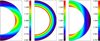 |
Fig. 1. Color-coded contours of the rotation law due to the Λ effect with V(0) = −1, V(1) = 0 and H(1) = 1 (left), H(1) = 0 (middle), H(1) = −1 (right). Meridional circulation and the off-diagonal eddy viscosity are artificially suppressed. Positive H(1) values lead to solar-type equatorial acceleration while negative H(1) values lead to antisolar rotation profiles ν⊥ = 0. |
The question remains as to how the meridional circulation would modifiy these results if it were included. The above finding that formally negative H easily produces antisolar rotation profiles remains true if the meridional circulation due to radial shear is also taken into account. The vorticity of the circulation depends on the sign of the radial shear ∂Ω/∂r. At the surface it flows towards the equator for superrotation and towards the poles for subrotation (Kippenhahn 1963). On the other hand, a circulation which flows towards the equator at the surface of the convection zone (“clockwise flow”) produces differential rotation with an accelerated equator while it produces a polar vortex if it flows towards the poles (“counterclockwise flow”). One takes from Fig. 2 (top) that for all choices of H(1) the meridional circulation flows counterclockwise in the northern hemisphere, reducing the equatorial acceleration (left panel) or amplifying equatorial deceleration (right panel). Indeed, with circulation included, the bottom left plot of Fig. 2 with H(1) > 0 represents a model for convection zones with solar-type rotation laws, while the right panel of Fig. 2 with H(1) < 0 represents an antisolar rotation law. As the middle plots of Fig. 2 show, a meridional circulation towards the poles even produces a weak antisolar rotation without any Λ effect. Typically, as a result of the Taylor-Proudman theorem the isolines of the angular velocity Ω (with meridional flow included) become cylindrical. This effect appears in all plots of the bottom row of Fig. 2 but it is most prominent for H(1) < 0 which even without circulation generates cylinder-like Ω-isolines. Simultaneously, for rotation laws with small ∂Ω/∂z the amplitude of the circulation sinks.
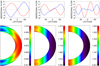 |
Fig. 2. Top: meridional circulation (given as its Reynolds numbers) at the top (blue) and bottom (red) of the convection zone associated with rotation laws shown in Fig. 1. Negative values at the surface of the northern hemisphere indicate a circulation pattern directed towards the poles (counterclockwise flow). Bottom: similar to Fig. 1 but with meridional circulation included. Positive H(1) values lead to solar-type acceleration of the equator (left panel). The (slow) counterclockwise meridional flow H(1) = 0 leads to a weak antisolar-type equatorial deceleration (middle panel). The right panels of Figs. 1 and 2 formally demonstrate the possibility of antisolar rotation laws to produce antisolar rotation laws with negative H(1). |
Several analytical studies of the Λ effect led to positive H(1), that is, cos θQθϕ > 0, for rigid rotation. Also, numerical simulations of rotating convection (Hupfer et al. 2006) or driven anisotropic turbulence under the influence of solid-body rotation (Käpylä 2019a) provide transport of angular momentum towards the equator. Earlier, Chan (2001) found transport towards the equator only for fast rotation while for slow rotation occasionally the opposite result appeared. Simulations by Rüdiger et al. (2005a) of rotating turbulent convection with much higher resolution provided very small Qθϕ for slow rotation and large positive Qθϕ for fast rotation. There seemed to be no hope, therefore, of explaining antisolar rotation laws for rotating stars with a hydrodynamical theory of turbulent rotating flows. In this paper numerical simulations of rotating convection in boxes are presented providing transport of angular momentum towards the poles for slow rotation. This transport towards the poles, however, does not result from the Λ effect but is due to the rotation-induced off-diagonal viscosity term ν⊥ in (5) in connection with a subrotation law ∂Ω/∂r < 0 which appears for slow rotation (Viviani et al. 2018). For solar-like convection zones with rotation profiles quasi-uniform in radius and rotating with the present-day solar rotation rate the ν⊥ term does not play any role.
3. Rotating convection
We perform simulations for convection with a fixed ordinary Prandtl number Pr = ν/χ with χ being the thermal diffusion coefficient. For stellar material the heat conductivity χ strongly exceeds the other diffusivities. Also the Roberts number q = χ/η with η as the microscopic magnetic resistivity is therefore much larger than unity. For numerical reasons we must work with the approximate surface value Pr = 0.1.
The simulations are done with the NIRVANA code by Ziegler (2002), which uses a conservative finite volume scheme in Cartesian coordinates. The length scale is defined by the depth of the convectively unstable layer. Periodic boundary conditions are formulated in the horizontal plane. The upper and lower boundaries are impenetrable and stress-free. The initial state is convectively unstable in a layer that occupies half of the box. Convection sets in if the Rayleigh number exceeds its critical value. In the dimensionless units the size of the simulation box is 2 × 6 × 6 in the x, y, and z directions, respectively. The lower and upper boundaries of the unstably stratified layer are located at x = 0.8 and x = 1.8, respectively. The numerical resolution is 128 × 384 × 384 grid points. The stratification of density, pressure, and temperature is piecewise polytropic, similar to that used in Rüdiger et al. (2012). The density varies by a factor five over the depth of the box, hence the density scale height is 1.2.
The code solves the momentum equation,
 (10)
(10)
where ρ is the mass density, u the gas velocity, p the gas pressure, g gravity, and Ω the rotation vector, in a corotating Cartesian box under mass conservation,
 (11)
(11)
together with the energy equation,
 (12)
(12)
where Fcond = −κ∇T being the conductive heat flux with the heat conduction coefficient κ. The viscosity tensor is
 (13)
(13)
and the total energy e = U + ρu2/2 is the sum of the thermal and kinetic energy densities. An ideal gas with a constant mean molecular weight μ = 1 is considered, hence
 (14)
(14)
for the thermal energy density with ℛ the gas constant and γ = cp/cv = 5/3. The gas is kept at a fixed temperature at the bottom and a fixed heat flux at the top of the simulation box. More technical details including the boundary conditions have been described in Rüdiger et al. (2012).
Figure 3 gives the auto-correlations of the one-point correlation tensor (3) for convection that is subject to slow and fast rotation. The colatitude is θ = 45°. As expected, the horizontal turbulent intensities are identical for slow rotation while the vertical intensity  has the dominating value. The latter is strongly suppressed by faster rotation (the radial turbulence intensity is reduced by more than a factor of two for Ω = 30) while there is almost no visible suppression of the horizontal components.
For driven turbulence in a quasilinear approximation we have
 (15)
(15)
with
 (16)
(16)
(Rüdiger 1989). The sign of the expressions follows from the form of the positive-definite spectrum E(k, ω) and is obviously negative for white-noise spectra but is positive for spectral functions which are sufficiently steep in ω. Also for the maximally steep spectrum such as δ(ω) the ε is positive, describing a rotational quenching of the turbulence intensities.
The vector of rotation at the colatitude θ is Ω = Ω(cosθ, −sinθ, 0), so that Eq. (15) gives
 (17)
(17)
The rotational quenching of the radial turbulence intensity shown in Fig. 3 can be described by Eq. (17) with ε > 0.
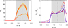 |
Fig. 3. Convection of slow rotation (Ω = 1, solid lines) and fast rotation (Ω = 30, dashed lines). Left: Qrr, right: Qθθ (red lines) and Qϕϕ (blue lines). The gray-shaded area indicates the convectively unstable part with the vertical dashed line showing its center and d is the thickness of the convectively unstable layer. Correlations Qrr, Qθθ, and Qϕϕ and rotation rates Ω are given in code units. The volume-averaged turbulence intensity is |

Another direct consequence of (15) is the existence of the cross-correlation of radial and latitudinal fluctuations, that is,
 (18)
(18)
which vanishes at the poles and the equator by definition. In a sense, the correlation Qrθ mimics the turbulent thermal conductivity tensor. If a radial temperature gradient exists, a negative cross-correlation Qrθ organizes heat transport to the poles resulting in a meridional circulation towards the equator at the surface (Rüdiger et al. 2005b).
For positive ε, the rotation-induced cross-correlation Qrθ after (18) becomes negative. This theoretical result complies with the results of numerical simulations (Käpylä 2019a). The expression (15) only describes the rotational influence on isotropic turbulence. Rüdiger et al. (2005a) also considered the rotational influence on turbulence fields which are anisotropic in the radial direction with the general result that Qrθ is always less than zero (northern hemisphere) for steep spectra E and for all rotation rates.
Hereafter we switch to the Cartesian box coordinates x (representing the radial coordinate r), y (representing the colatitude θ), and z (representing the azimuth ϕ) hence Qrθ → Qxy, Qrϕ → Qxz and Qθϕ → Qyz. The shears r∂Ω/∂r and ∂Ω/∂θ translate into dUz/dx and dUz/dy, respectively. After averaging over the horizontal (yz) plane the relations (4) and (5) turn into
 (19)
(19)
and
 (20)
(20)
The cross-correlation (18) completed by the viscosity term becomes
 (21)
(21)
The attention is focused here on the influence of the diffusion terms in Eqs. (20) and (21) in order to probe the existence of the viscosities ν‖ and ν⊥ by simulations. To this end the rotation rates are assumed to be so small that the nondiffusive terms in the relations (20) and (21) for the cross-correlations are negligible. The second term in Eq. (21) is positive for outwards decreasing meridional flow Uy, for example. Consequently, the cross-correlation Qxy should be positive for slow rotation and negative for rapid rotation, changing the sign at a certain value of the parameter Ω (which denotes the angular velocity Ω of the rotation in code units). One finds such a transition from positive to negative values for 5 < Ω < 10 in the simulations given in Fig. 4. The coincidence suggests that indeed the influence of viscosity terms in the expressions of cross-correlations may lead to direction reversals of transport terms as a function of rotation.
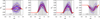 |
Fig. 4. Snapshots of the radial profiles of the radial cross-correlation |


Without rotation, all cross-correlations vanish. For the slow-rotation models with Ω = 1, already finite values appear (left plots in Figs. 4 and 5). At the radial boundaries the correlations Qxy and Qxz vanish by the boundary condition (ux = 0) but the horizontal cross-correlation Qyz remains finite; it is always positive at the top and bottom of the unstable box which indicates H > 0 if a possible mean circulation Uz were maximal or minimal at the top or bottom of the convection box (as it is, see Fig. 6).
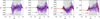 |
Fig. 5. Similar to Fig. 4 but for the horizontal cross-correlation |

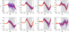 |
Fig. 6. Radial profiles of the meridional flow Uy (top) and zonal flow Uz (bottom) in the convective box (shaded). The parameters are Ω = 1, Ω = 3, Ω = 5, and Ω = 10 (from left to right). The circulation is always counterclockwise and the rotation is decelerated at the surface (subrotation). Pr = 0.1, θ = 45°. |
The correlation Qxy for slow rotation is positive so that heat is transported towards the equator. At the same time the horizontal correlation Qyz assumes negative values. Independent of the rotation rates and for both hemispheres we find the general result that always QxyQyz < 0. The simulations therefore show that angular momentum flux to the equator (poles) is always accompanied by heat transport to the poles (equator). Somewhere between Ω = 5 and Ω = 10 the cross-correlations Qxy and Qyz change their signs becoming negative (Qxy) and positive (Qyz) for fast rotation. These signs are well-known from the analytical expressions derived for driven turbulence for fast rotation. In this case, the angular momentum is transported inward as well as toward the equator by the convection; in other words, it flows along cylindric surfaces.
For increasingly fast rotation the amplitudes of the negative Qxy are increasing, contrary to Qyz which decrease. This is a basic difference for the two cross-correlations. We note that for the transformation Ω → −Ω the correlations Qyz change their sign which is not the case for Qxy. The reason is that Qxy is even in the rotational rate Ω while the horizontal cross-correlation Qyz is odd.
4. The eddy viscosities
Equation (18) neglects the influence of a possible radial shear dUy/dx of a meridional flow. The question is whether large-scale mean flow characterizes the simulation box as in the simulations of Chan (2001) and Käpylä et al. (2004), which could be used to calculate the eddy viscosities after relations (20) and (21). The mean flows in the box have been calculated for slow rotation. The top panel of Fig. 6 gives flows in the meridional direction and the bottom panel gives zonal flows in the azimuthal direction. The basic rotation there has been varied from Ω = 1 to Ω = 10 and the Prandtl number is fixed at Pr = 0.1. The following estimate concerns the first example with Ω = 1 with the cross-correlation Qxy ≃ 0.01 (from Fig. 5) and the shear δUy/δx ≃ −0.2 (from Fig. 6). The standard eddy viscosity ν‖ ≃ 1.5 in code units for slow rotation. The microscopic viscosity of the model in the same units is ν = 6 × 10⁻³, meaning that ν‖/ν ≃ 240. One finds very similar values for Ω = 3.
The dimensionless eddy viscosity αvis, following
 (22)
(22)
may also be introduced which is often assumed in turbulence research to be αvis ≃ 0.3. To find the correlation time τcorr an auto-correlation analysis as done by Küker & Rüdiger (2018) is necessary. The result is τcorr ≃ 0.1 in code units, hence αvis ≲ 0.5 which indeed is of the expected order of magnitude.
Figure 6 also demonstrates that the negative shear dUy/dx is always accompanied by a negative shear dUz/dx of the zonal flow, hence dUy/dx · dUz/dx > 0. Transformed to the global system, this means that a subrotating shell generates a counterclockwise circulation where the fluid drifts towards the poles at the surface. This type of flow pattern has already been described in the text below Eq. (8). On the other hand, the existence of Uz allows us to estimate the off-diagonal viscosity after Eq. (20) with H ≈ 0 for Ω = 1 or Ω = 3 to ν⊥ ≃ 0.05, hence ν⊥/ν‖ ≃ 0.03 in code units or  in physical units.
Following Eqs. (19) and (20), the shear dUz/dx contributes to the cross-correlations Qxz and Qyz. Because of its negativity, the viscosity term in (19) is positive, meaning that the actual value of |V| is even larger than indicated by Qxz from the simulations.
4.1. Rotation-induced off-diagonal eddy viscosity
The same radial velocity gradient appears in the expression for the horizontal cross-correlation in a higher order of the rotation rate. The two viscosities in (20) can be expressed by the integrals
 (23)
(23)
and
 (24)
(24)
(Rüdiger 1989). The ratio  is a dimensionless number. Not surprisingly, the first integral is positive definite. On the other hand, the second integral is positive for all other monotonously decreasing spectra in line with the following expression:
 (25)
(25)
The integral in (24) is even positive for spectra of the white-noise-type. To demonstrate this point, we evaluate the frequency integral with uniform E. As
 (26)
(26)
here the ν⊥ is also positive. We note however that very steep spectra such as δ(ω) lead to vanishing ν⊥ which explains the absence of antisolar rotation laws in the calculations based on that turbulence model (Kitchatinov et al. 1994). It therefore seems likely that observations of slowly rotating stars with a decelerated equator question the application of turbulences with δ-like frequency spectra in stellar convection models. The steepest frequency spectra describe fluids in the high-viscosity limit (low Reynolds number of the fluctuations) while spectra with a quasi-white-noise behavior belong to the inviscid approximation (large Reynolds number of the fluctuations). As the corresponding integral for the standard eddy viscosity (23) is π/2 one obtains, for rather flat spectra,  with Re the Reynolds number of the fluctuations.
If ν⊥ > 0 and dUz/dx < 0 (see Fig. 6) negative contributions to the horizontal cross-correlation are produced. The existence of the off-diagonal viscosity ν⊥ therefore explains the resulting negativity of the cross-correlation Qyz for slow rotation. The result confirms the above finding that all values of Qyz are positive at the top and bottom boundaries where the mean shear vanishes. For faster rotation, the increasing positive values of H overcompensate the negative contribution from the radial shear of Uz which becomes increasingly unimportant. The transition from negative to positive Qyz happens in Fig. 5 for Ω ≃ 5. Figure 6 also demonstrates that the shear dUz/dx grows for Ω < 5 and overcompensates the positive H term producing the obtained negative cross-correlations.
As the mechanisms of the null crossings of Qxy and Qyz are different, the values for the critical Ω should not be identical for both cases.
4.2. Antisolar rotation
Models are considered of such slow rotation that H ≃ 0 and a (negative) V(0) exists in addition to the rotation-induced off-diagonal viscosity ν⊥. The existence of the latter has been indicated by the simulations for the horizontal cross-correlation Qyz shown in Fig. 5. This leads to functions of H that are formally negative (for slow rotation) for which Fig. 1 demonstrates the appearance of antisolar rotation laws. The off-diagonal element ν⊥ is varied in Fig. 7 from ν⊥ = −0.5 (left panel) through zero (middle panel) to ν⊥ = 0.5 (right panel). For the models shown in the top row of the plots the resulting meridional circulation is artificially suppressed. One finds that negative V(0) always produces rotation laws with negative radial shear, which in combination with positive ν⊥ leads to antisolar rotation and vice versa. Hence, for V(0)ν⊥ < 0 the equator rotates slower than the polar regions and just this condition is the result of the given numerical simulations. One could also demonstrate that the equator is accelerated for V(0)ν⊥ > 0 (not shown). The examples in the top row of Fig. 7 (from left to right) clearly demonstrate how the completion of the eddy viscosity tensor with the (positive) off-diagonal term ν⊥ leads to the cylindric geometry of the Ω isolines required by the Taylor-Proudman theorem – without any help of the meridional circulation.
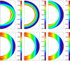 |
Fig. 7. Similar to Fig. 1 but for slow rotation (V(0) = −1 and V(1) = H(1) = 0). The off-diagonal viscosity term varies from ν⊥ = −0.5 (left), through ν⊥ = 0 (middle), to ν⊥ = 0.5 (right). Meridional circulation is suppressed (top) or it is included as in Fig. 2 (bottom). For positive ν⊥ the rotation is always antisolar without and with meridional circulation. The circulation is counterclockwise. We note the negative radial shear below the equator in all cases. |
If the associated meridional flow is also allowed to transport angular momentum, as done in the models in the second row of Fig. 7, all the Ω isolines become cylindrical in accordance with the Taylor-Proudman theorem and the antisolar rotation law is only modified but not destroyed. We note how in the middle panels only the meridional circulation changes the type of the rotation law from uniform on spherical shells to cylindrical with respect to the rotation axis. The circulation cells always flow counterclockwise towards the poles at the surface.
From the comparison of Figs. 1 and 7 one finds that antisolar rotation profiles result both for positive ν⊥ in common with subrotation and/or for negative H(1). The latter can be excluded with numerical experiments where Uy and Uz are artificially suppressed mimicking the existence of strict solid-body rotation. This has been confirmed by PENCIL CODE4 simulations which use the same setup as in Käpylä (2019b).
Figure 8 presents the results from a slowly rotating run with and without mean flows. The used Coriolis number Co = Ωd/πurms ≈ 0.25 corresponds to Ω ≃ 4 in NIRVANA code units. We find that the signs of Qxy and Qyz change when the mean flows are suppressed. This is consistent with a dominating contribution from turbulent viscosity in Qxy and the rotation-induced off-diagonal viscosity term in Qyz in accordance with the above theory. Without shear the cross-correlation Qyz (equivalent to Qθϕ in spherical coordinates) is always positive and the cross-correlation Qxy (equivalent to Qrθ in spherical coordinates) is always negative.
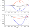 |
Fig. 8. Normalized off-diagonal Reynolds stresses as indicated by the legends from runs with (upper panel) and without (below) horizontal mean flows. The vertical dotted lines indicate the top and bottom of the convection zone. |
Let us finally note that the negative value of Qxz (equivalent to Qrϕ in spherical coordinates) clearly becomes more negative in the case where the shear is suppressed, indicating a strong contribution from the term involving ν‖; see Eq. (19).
5. Discussion
The cross-correlations Qrθ, Qrϕ, and Qθϕ of the fluctuating velocities in a rotating turbulence are playing basic roles in understanding the rotation laws of stars with outer convection zones. Briefly, the tensor component Qrθ transports thermal energy in the latitudinal direction (“warm poles”) while Qrϕ and Qθϕ transport angular momentum in the radial and meridional directions. For driven turbulence of a uniformly rotating density-stratified medium (stratified in the radial direction) the correlations fulfill simple sign rules independent of the rotation rate: it is Qrθ < 0, Qrϕ < 0 and Qθϕ > 0, taken always in the northern hemisphere. In physical quantities this means that thermal energy is transported to the poles while the angular momentum is transported inward and towards the equator. The resulting warm poles drive a clockwise meridional circulation (northern hemisphere) which together with the positive Qθϕ transports angular momentum towards the equator. Hence, if the convection zone can be modelled by driven turbulence under fast global rotation then the resulting surface rotation law will always be of the solar-type. The simultaneous solution of the Reynolds equation and the corresponding energy equation provides rotation profiles, meridional circulation patterns, and pole–equator temperature differences that are relatively close to observations (Kitchatinov & Rüdiger 1999; Küker et al. 2011). The results are similar for all rotation rates and the number of tuning parameters is low.
There are, however, increasing observational indications for the existence of antisolar rotation laws where the equator rotates slower than the polar regions. The results of observations (Metcalfe et al. 2016) as well as of numerical simulations (Gastine et al. 2014; Viviani et al. 2018) suggest that stars with slow rotation possess antisolar rotation laws. Based on photometric Kepler/K2 data from the open cluster M 67, Brandenburg & Giampapa (2018) also argue in favor of the appearance of antisolar rotation laws for slow rotators with large Rossby numbers.
We assume that because of the often-stated positivity of the function H the horizontal Λ effect always transports angular momentum towards the equator in favor of an accelerated equator. If, however, a rotation law with a negative radial gradient exists then the rotation-induced off-diagonal components of the eddy viscosity tensor such as ν⊥ transport angular momentum towards the poles in favor of a polar vortex (“antisolar”). This also implies that a strictly radius-dependent rotation law Ω = Ω(r) can never exist in (slowly) rotating convection zones. After the Taylor-Proudman theorem, the rotation will tend to produce z-independent rotation laws, and therefore a negative radial shear of the angular velocity is always accompanied by slightly accelerated polar regions.
We compute the cross-correlations Qrθ, Qrϕ, and Qθϕ from numerical simulations of convection in a rotating box. The averaging process concerns the horizontal planes, hence only radial shear can influence the cross-correlations (see Eqs. (4), (5), and (21)). For fast rotation, the well-known findings of positive Qθϕ and negative Qrθ, Qrϕ are reproduced (northern hemisphere). For slow rotation however, the signs of both Qrθ and Qθϕ change almost simultaneously, meaning that the angular momentum is now transported to the poles and the heat is transported to the equator. The resulting warm equator leads to a counterclockwise meridional circulation which also transports the angular momentum to the poles. The new signs of the quantities Qrθ and Qθϕ may thus lead to antisolar differential rotation.
This behavior, however, is due to the appearance of large-scale flows in zonal and in meridional directions. The zonal flow Uz mimics differential rotation with negative radial gradient. Via the off-diagonal viscosity in Eq. (5), for positive ν⊥, a negative contribution to Qθϕ leads to overcompensation of the positive but small values of H. A similar effect happens for Qrθ where the negative radial gradient of Uy combined with the positive eddy viscosity ν‖ provides positive contributions to the negative cross-correlation (18).
From the associated numerical values, with Eq. (22) ν‖ can be calculated leading to ν‖/ν ≃ 240, or to the (reasonable) dimensionless quantity αvis ≲ 0.5. The simulations for slow rotation lead to  for the ratio of the rotation-induced off-diagonal viscosity term and the standard diagonal eddy viscosity.
We also studied the influence of the radial shears of the large-scale flows Uy and Uz on the cross-correlations Qxy and Qyz with numerical experiments where the Uy and Uz can artificially be suppressed. In these cases, for all rotation rates, the calculations led to negative Qxy and positive Qyz. Without large-scale flows the analytical results are confirmed, namely that always Qrθ < 0 and Qθϕ > 0 for the northern hemisphere formulated in spherical coordinates. For slow rotation, both signs are changed if the large-scale radial shear flows are allowed to back-react.
In summary, we show that a so-far neglected rotation-induced off-diagonal eddy viscosity term combined with rotation laws with a negative radial gradient (subrotation, as existing in slowly rotating stars) is able to produce differential rotation of the antisolar type. This result complies with the (numerical) findings of Viviani et al. (2018) that negative radial Ω-gradients and antisolar differential rotation are closely related. Therefore, if new observations confirm the existence of decelerated equators at the surface of slowly rotating stars then we shall better understand the nature of the active eddy viscosity tensor and also the underlying turbulence model in its low- or high-viscosity limit.
ν‖ = ν1 ≡ νT in the notation of Kitchatinov et al. (1994).
ν⊥ = ν2 in the notation of Kitchatinov et al. (1994).
In the linear-in-Ω approximation by Kippenhahn (1963) a very similar mechanism is realized via meridional flow.
Acknowledgments
PJK acknowledges the computing resources provided by CSC – IT Center for Science, who are administered by the Finnish Ministry of Education; of Espoo, Finland, and the Gauss Center for Supercomputing for the Large-Scale computing project “Cracking the Convective Conundrum” in the Leibniz Supercomputing Centre’s SuperMUC supercomputer in Garching, Germany. This work was supported in part by the Deutsche Forschungsgemeinschaft Heisenberg programme (grant No. KA 4825/1-1; PJK) and the Academy of Finland ReSoLVE Centre of Excellence (grant No. 307411; PJK).
References
- Barnes, J. R., Collier Cameron, A., Donati, J. F., et al. 2005, in 13th Cambridge Workshop on Cool Stars, Stellar Systems and the Sun, eds. F. Favata, G. A. J. Hussain, & B. Battrick, ESA Spec. Publ., 560, 95 [NASA ADS] [Google Scholar]
- Bazot, M., Benomar, O., Christensen-Dalsgaard, J., et al. 2019, A&A, 623, A125 [NASA ADS] [CrossRef] [EDP Sciences] [Google Scholar]
- Benomar, O., Bazot, M., Nielsen, M. B., et al. 2018, Science, 361, 1231 [Google Scholar]
- Brandenburg, A., & Giampapa, M. S. 2018, ApJ, 855, L22 [NASA ADS] [CrossRef] [Google Scholar]
- Brun, A. S., & Palacios, A. 2009, ApJ, 702, 1078 [NASA ADS] [CrossRef] [Google Scholar]
- Chan, K. L. 2001, ApJ, 548, 1102 [NASA ADS] [CrossRef] [Google Scholar]
- Donati, J.-F., & Collier Cameron, A. 1997, MNRAS, 291, 1 [NASA ADS] [CrossRef] [Google Scholar]
- Featherstone, N. A., & Miesch, M. S. 2015, ApJ, 804, 67 [NASA ADS] [CrossRef] [Google Scholar]
- Gastine, T., Morin, J., Duarte, L., et al. 2013, A&A, 549, L5 [NASA ADS] [CrossRef] [EDP Sciences] [Google Scholar]
- Gastine, T., Yadav, R. K., Morin, J., Reiners, A., & Wicht, J. 2014, MNRAS, 438, L76 [NASA ADS] [CrossRef] [Google Scholar]
- Gilman, P. A. 1977, Geophys. Astrophys. Fluid Dyn., 8, 93 [NASA ADS] [CrossRef] [Google Scholar]
- Guerrero, G., Smolarkiewicz, P. K., Kosovichev, A. G., & Mansour, N. N. 2013, ApJ, 779, 176 [NASA ADS] [CrossRef] [Google Scholar]
- Hathaway, D. H., Upton, L., & Colegrove, O. 2013, Science, 342, 1217 [NASA ADS] [CrossRef] [Google Scholar]
- Hupfer, C., Käpylä, P. J., & Stix, M. 2006, A&A, 459, 935 [NASA ADS] [CrossRef] [EDP Sciences] [Google Scholar]
- Käpylä, P. J. 2019a, A&A, 622, A195 [NASA ADS] [CrossRef] [EDP Sciences] [Google Scholar]
- Käpylä, P. J. 2019b, A&A, submitted [arXiv:1812.07916] [Google Scholar]
- Käpylä, P. J., Korpi, M. J., & Tuominen, I. 2004, A&A, 422, 793 [NASA ADS] [CrossRef] [EDP Sciences] [Google Scholar]
- Käpylä, P. J., Mantere, M. J., & Brandenburg, A. 2011, Astron. Nachr., 332, 883 [NASA ADS] [CrossRef] [Google Scholar]
- Käpylä, P. J., Käpylä, M. J., & Brandenburg, A. 2014, A&A, 570, A43 [NASA ADS] [CrossRef] [EDP Sciences] [Google Scholar]
- Kővári, Z., Oláh, K., Kriskovics, L., et al. 2017, Astron. Nachr., 338, 903 [Google Scholar]
- Kippenhahn, R. 1963, ApJ, 137, 664 [NASA ADS] [CrossRef] [Google Scholar]
- Kitchatinov, L. L., & Olemskoy, S. V. 2011, MNRAS, 411, 1059 [NASA ADS] [CrossRef] [Google Scholar]
- Kitchatinov, L. L., & Rüdiger, G. 1999, A&A, 344, 911 [NASA ADS] [Google Scholar]
- Kitchatinov, L. L., & Rüdiger, G. 2004, Astron. Nachr., 325, 496 [NASA ADS] [CrossRef] [Google Scholar]
- Kitchatinov, L. L., Pipin, V. V., & Rüdiger, G. 1994, Astron. Nachr., 315, 157 [NASA ADS] [CrossRef] [Google Scholar]
- Küker, M., & Rüdiger, G. 2018, Astron. Nachr., 339, 447 [NASA ADS] [CrossRef] [Google Scholar]
- Küker, M., Rüdiger, G., & Kitchatinov, L. L. 2011, A&A, 530, A48 [NASA ADS] [CrossRef] [EDP Sciences] [Google Scholar]
- Künstler, A., Carroll, T. A., & Strassmeier, K. G. 2015, A&A, 578, A101 [NASA ADS] [CrossRef] [EDP Sciences] [Google Scholar]
- Metcalfe, T. S., Egeland, R., & van Saders, J. 2016, ApJ, 826, L2 [Google Scholar]
- Reinhold, T., & Arlt, R. 2015, A&A, 576, A15 [NASA ADS] [CrossRef] [EDP Sciences] [Google Scholar]
- Reinhold, T., Reiners, A., & Basri, G. 2013, A&A, 560, A4 [NASA ADS] [CrossRef] [EDP Sciences] [Google Scholar]
- Rüdiger, G. 1989, Differential Rotation and Stellar Convection. Sun and the Solar Stars (Berlin: Akademie Verlag) [Google Scholar]
- Rüdiger, G., Egorov, P., & Ziegler, U. 2005a, Astron. Nachr., 326, 315 [NASA ADS] [CrossRef] [Google Scholar]
- Rüdiger, G., Egorov, P., Kitchatinov, L. L., & Küker, M. 2005b, A&A, 431, 345 [NASA ADS] [CrossRef] [EDP Sciences] [Google Scholar]
- Rüdiger, G., Küker, M., & Schnerr, R. S. 2012, A&A, 546, A23 [NASA ADS] [CrossRef] [EDP Sciences] [Google Scholar]
- Solanki, S. K. 2003, A&ARv, 11, 153 [Google Scholar]
- Strassmeier, K. G. 2009, A&ARv, 17, 251 [NASA ADS] [CrossRef] [Google Scholar]
- Viviani, M., Warnecke, J., Käpylä, M. J., et al. 2018, A&A, 616, A160 [NASA ADS] [CrossRef] [EDP Sciences] [Google Scholar]
- Viviani, M., Käpylä, M. J., Warnecke, J., Käpylä, P. J., & Rheinhardt, M. 2019, ApJ, accepted [arXiv:1902.04019] [Google Scholar]
- Warnecke, J., Käpylä, P. J., Mantere, M. J., & Brandenburg, A. 2013, ApJ, 778, 141 [NASA ADS] [CrossRef] [Google Scholar]
- Wöhl, H., Brajša, R., Hanslmeier, A., & Gissot, S. F. 2010, A&A, 520, A29 [NASA ADS] [CrossRef] [EDP Sciences] [Google Scholar]
- Ziegler, U. 2002, A&A, 386, 331 [NASA ADS] [CrossRef] [EDP Sciences] [Google Scholar]
All Figures
|
Fig. 1. Color-coded contours of the rotation law due to the Λ effect with V(0) = −1, V(1) = 0 and H(1) = 1 (left), H(1) = 0 (middle), H(1) = −1 (right). Meridional circulation and the off-diagonal eddy viscosity are artificially suppressed. Positive H(1) values lead to solar-type equatorial acceleration while negative H(1) values lead to antisolar rotation profiles ν⊥ = 0. |
| In the text | |
|
Fig. 2. Top: meridional circulation (given as its Reynolds numbers) at the top (blue) and bottom (red) of the convection zone associated with rotation laws shown in Fig. 1. Negative values at the surface of the northern hemisphere indicate a circulation pattern directed towards the poles (counterclockwise flow). Bottom: similar to Fig. 1 but with meridional circulation included. Positive H(1) values lead to solar-type acceleration of the equator (left panel). The (slow) counterclockwise meridional flow H(1) = 0 leads to a weak antisolar-type equatorial deceleration (middle panel). The right panels of Figs. 1 and 2 formally demonstrate the possibility of antisolar rotation laws to produce antisolar rotation laws with negative H(1). |
| In the text | |
|
Fig. 3. Convection of slow rotation (Ω = 1, solid lines) and fast rotation (Ω = 30, dashed lines). Left: Qrr, right: Qθθ (red lines) and Qϕϕ (blue lines). The gray-shaded area indicates the convectively unstable part with the vertical dashed line showing its center and d is the thickness of the convectively unstable layer. Correlations Qrr, Qθθ, and Qϕϕ and rotation rates Ω are given in code units. The volume-averaged turbulence intensity is |
| In the text | |
|
Fig. 4. Snapshots of the radial profiles of the radial cross-correlation |
| In the text | |
|
Fig. 5. Similar to Fig. 4 but for the horizontal cross-correlation |
| In the text | |
|
Fig. 6. Radial profiles of the meridional flow Uy (top) and zonal flow Uz (bottom) in the convective box (shaded). The parameters are Ω = 1, Ω = 3, Ω = 5, and Ω = 10 (from left to right). The circulation is always counterclockwise and the rotation is decelerated at the surface (subrotation). Pr = 0.1, θ = 45°. |
| In the text | |
|
Fig. 7. Similar to Fig. 1 but for slow rotation (V(0) = −1 and V(1) = H(1) = 0). The off-diagonal viscosity term varies from ν⊥ = −0.5 (left), through ν⊥ = 0 (middle), to ν⊥ = 0.5 (right). Meridional circulation is suppressed (top) or it is included as in Fig. 2 (bottom). For positive ν⊥ the rotation is always antisolar without and with meridional circulation. The circulation is counterclockwise. We note the negative radial shear below the equator in all cases. |
| In the text | |
|
Fig. 8. Normalized off-diagonal Reynolds stresses as indicated by the legends from runs with (upper panel) and without (below) horizontal mean flows. The vertical dotted lines indicate the top and bottom of the convection zone. |
| In the text | |
Current usage metrics show cumulative count of Article Views (full-text article views including HTML views, PDF and ePub downloads, according to the available data) and Abstracts Views on Vision4Press platform.
Data correspond to usage on the plateform after 2015. The current usage metrics is available 48-96 hours after online publication and is updated daily on week days.
Initial download of the metrics may take a while.