| Issue |
A&A
Volume 630, October 2019
|
|
|---|---|---|
| Article Number | A82 | |
| Number of page(s) | 10 | |
| Section | Planets and planetary systems | |
| DOI | https://doi.org/10.1051/0004-6361/201834413 | |
| Published online | 24 September 2019 | |
Quasi-static contraction during runaway gas accretion onto giant planets
1
Lund Observatory, Department of Astronomy and Theoretical Physics, Lund University,
Box 43,
22100
Lund,
Sweden
e-mail: michiel@astro.lu.se
2
Université Côte d’Azur, Observatoire de la Côte d’Azur, CNRS, Laboratoire Lagrange, Bd de l’Observatoire,
CS 34229,
06304
Nice Cedex 4,
France
3
Astronomy Unit, Queen Mary University of London,
Mile End Road,
London,
E1 4NS,
UK
4
Institut Universitaire de France,
103 Boulevard Saint-Michel,
75005
Paris,
France
Received:
10
October
2018
Accepted:
14
July
2019
Gas-giant planets, like Jupiter and Saturn, acquire massive gaseous envelopes during the approximately 3 Myr-long lifetimes of protoplanetary discs. In the core accretion scenario, the formation of a solid core of around ten Earth masses triggers a phase of rapid gas accretion. Previous 3D grid-based hydrodynamical simulations found that runaway gas accretion rates correspond to approximately 10 to 100 Jupiter masses per Myr. Such high accretion rates would result in all planets with larger than ten Earth-mass cores to form Jupiter-like planets, which is in clear contrast to the ice giants in the Solar System and the observed exoplanet population. In this work, we used 3D hydrodynamical simulations, that include radiative transfer, to model the growth of the envelope on planets with different masses. We find that gas flows rapidly through the outer part of the envelope, but this flow does not drive accretion. Instead, gas accretion is the result of quasi-static contraction of the inner envelope, which can be orders of magnitude smaller than the mass flow through the outer atmosphere. For planets smaller than Saturn, we measured moderate gas accretion rates that are below one Jupiter mass per Myr. Higher mass planets, however, accrete up to ten times faster and do not reveal a self-driven mechanism that can halt gas accretion. Therefore, the reason for the final masses of Saturn and Jupiter remains difficult to understand, unless their completion coincided with the dissipation of the solar nebula.
Key words: planets and satellites: formation / planets and satellites: gaseous planets / hydrodynamics / methods: numerical
© ESO 2019
1 Introduction
Giant planets acquire their gaseous envelopes in a multi-stage process. When solid bodies grow more massive than the Earth, they start attracting thick envelopes from the surrounding hydrogen and helium gas in the protoplantary disc (Mizuno 1980). In this first phase, the ongoing accretion of solids provides sufficient heat to support the young atmosphere, which is less massive than the solid core it surrounds. However, as the planet grows larger, it can get isolated from the surrounding planetesimals (Kokubo & Ida 1998) and pebbles (Morbidelli & Nesvorny 2012; Lambrechts et al. 2014; Bitsch et al. 2018). Without solid accretion, compressional heating of the inner envelope becomes the dominant source of pressure support (Lambrechts & Lega 2017). As a consequence, a second phase is triggered where the envelope of the planet cools down. The luminosity decreases and the planet slowly gains in mass (Bodenheimer & Pollack 1986; Pollack et al. 1996). Interestingly, if the envelope mass grows sufficiently and becomes comparable to the core mass, this secular envelope cooling sequence would come to an end. Then, as shown by pioneering work from Mizuno (1980) and Stevenson (1982), the onset of self-gravity triggers a third phase of rapid gas accretion. It is this last epoch of atmosphere growth when envelopes undergo so-called runaway gas accretion, that is the focus of this work. We thus loosely use the term runaway gas accretion to describe gas accretion onto planets that stopped accreting solids and have an envelope mass comparable to or larger than the core mass.
The process of runaway gas accretion has been modelled in two different ways. Initially, 1D hydrostatic time-evolution models were created (Bodenheimer & Pollack 1986; Pollack et al. 1996) that are similar to those used for stellar evolution calculations. Later, multidimmensional hydrodynamical models of gas accretion became numerically feasible (Bryden et al. 1999; Kley 1999; Lubow et al. 1999; Ayliffe & Bate 2009).
Simplified 1D models assume planetary atmospheres that are in hydrostatic balance at all times (Ikoma et al. 2000; Papaloizou & Nelson 2005; Mordasini et al. 2012; Piso & Youdin 2014; Lee et al. 2014; Coleman et al. 2017). By calculating the luminosity, and hence the rate of heat loss, and by assuming the luminosity is sourced by the accretion of gas onto the planet, it becomes possible to integrate the model forward in time. These types of models consistently find that envelopes are comparable to the core mass when they start to rapidly accrete gas by quasi-static contraction. After solid accretion has come to a halt, gas accretion first proceeds slowly and then reaches rates around 10−3 ME yr−1 around Saturn-mass planets (Mordasini et al. 2012), under nominal conditions. Nevertheless, the simplifying nature of 1D calculations have made it difficult to draw firm conclusions. The approximation that these planets in 1D models are in perfect hydrostatic equilibrium all the way out to the edge of the envelope is the most limiting assumption.
Hydrodynamical models in 3D demonstrate that hydrostatic balance is a problematic assumption. Generally, protoplanetary discs easily provide gas to the Hill sphere around accreting cores, even when the planet starts carving a gap in the disc (Bryden et al. 1999; Kley 1999; Lubow et al. 1999). Therefore, at all times, gas can enter the envelope and dynamically interact with the planet. However, not all of this inflowing gas becomes bound to the planet. Indeed, previous studies around low-mass planets, where the envelope mass is smaller than the core mass, have shown that most of the gas that enters the Hill sphere is not accreted, but simply gets advected out of the envelope and redeposited in the disc (Tanigawa et al. 2012; Ormel et al. 2015a; Fung et al. 2015; Cimerman et al. 2017; Lambrechts & Lega 2017; Kurokawa & Tanigawa 2018; Popovas et al. 2018). Radiative simulations show that only the central envelope, which is shielded from this mass flux, accretes gas (D’Angelo & Bodenheimer 2013; Cimerman et al. 2017; Lambrechts & Lega 2017; Kurokawa & Tanigawa 2018).
Around higher mass planets, the situation remains unclear (Tanigawa & Watanabe 2002; D’Angelo et al. 2003; Machida et al. 2010; Gressel et al. 2013; Szulágyi et al. 2014). These studies report accretion rates much higher than 1D models, of the order of 10−2 to 10−1 ME yr−1 when planets enter the runaway regime. However, these rates were made under approximations to limit the numerical cost, such as the use of low resolution, the presence of an artificial sink-cell at the centre of the planet or restrictions on the equation of state, such as a constant temperature approach (Lubow et al. 1999; Tanigawa & Watanabe 2002; D’Angelo et al. 2003; Machida et al. 2010; Gressel et al. 2013). On the other hand, 3D radiative simulations using SPH (smoothed-particle hydrodynamics) reported slower accretion rates (Ayliffe & Bate 2009). However, these rates do not appear to be in agreement with 3D radiative hydrodynamical simulations by Szulágyi et al. (2016). In summary, the 1D and 3D gas accretion rates reported in the literature for the runaway gas accretion regime vary widely and the various simplifying assumptionsmake comparison difficult.
In this work, we measure gas accretion rates onto planets of various masses ranging from 15 to 330ME, using global 3D simulations that include radiative transfer. A full description of the methods can be found in Sect. 2. By limiting the integration times of our high resolution simulations to tens of orbits, we can measure quasi-steady gas accretion rates without evolving the gravitational potential in time. Based on these snapshot simulations, we argue that runaway gas accretion proceeds through quasi-static contraction, as discussed in Sect. 3. Initially, runaway gasaccretion is measured to be relatively slow, below a Jupiter mass per Myr. However, planets larger than Saturn accrete at rates that double their mass in less than 105 yr. Then, by combining the sequenceof measured accretion rates for given planetary masses, we trace the planetary mass as function of time, from the low-mass regime around 10ME up to masses of fully-formed giant planets larger than 100ME (Sect. 4). In this way, we argue that a planet can grow from approximately 10ME to a giant planet larger than 100ME in less than a 1 Myr. We subsequently discuss the implications of our findings on early and late formation scenarios for giant planets. We summarise our results in Sect. 5.
2 Methods
We numerically solve the hydrodynamical equations describing a planet embedded in an annulus of a protoplanetary disc, together with the equations of radiative transfer. A complete description of our methods can be found in Lambrechts & Lega (2017) and a detailed description of the FARGOCA code can be found in Lega et al. (2014).
This work differs from previous hydrodynamical works in two ways. Firstly, we do not employ a sink cell at the centre of our simulated planet removing mass or heat. Secondly, we solve for radiative transfer. This allows us to not belimited to isothermal numerics, which is important to correctly capture the atmosphere dynamics (Cimerman et al. 2017; Lambrechts & Lega 2017). In order to do so, we make use of the flux-limited diffusion approach (FLD, Levermore & Pomraning 1981) when solving the energy equation for both the thermal and radiative energy density (Bitsch et al. 2013). We use the ideal gas equation of state with an adiabatic index of γ = 1.4. For the opacity, we employ the prescription provided by Bell & Lin (1994) that covers the opacity provided by the gas and dust component of a gas with interstellar-medium composition and a solar dust-to-gas ratio of 0.01.
Simulation parameters.
2.1 Gravitational potential
A realistic gravitational potential is hard to obtain for high-mass planets. Like other studies, we employ a fixed potential for the planet, which does not take fully into account the self-gravity of an evolving envelope (Klahr & Kley 2006; Kley et al. 2009; Szulágyi et al. 2016). This approach is consistent with our aim of probing the runaway regime through a series of short time integrations around planets of increasing mass. Additionally, the gravitational potential requires artificial smoothing to avoid a too strong central mass concentration. For the smoothing length we used a constant fraction of the Hill sphere, rs = 0.2 rH or rs = 0.1 rH (see Table 1). Here, rH is the radius of the Hill sphere given by
 (1)
(1)
which corresponds to the maximal gravitational reach of the planet. At larger radii the tidal gravity force dominates. A detailed description of the potential can be found in Appendix A of Lambrechts & Lega (2017).
2.2 Disc set-up
We simulate a full annulus of the protoplanetary disc, in 3 dimensions. The width of the annulus can be found for each simulation in Table 1. To obtain sufficient resolution in the planetary atmosphere, we made use of a non-uniform grid (Lambrechts & Lega 2017). Additionally, we make use of mirror symmetry across the midplane to limit our simulations to the upper hemisphere. Table 1 lists the effective resolution for each of our simulations. A technical discussion of our numerical approach can be found in Appendix A.
We use nominal values for the disc parameters at the location of the planet at 5.1 AU. The disc gas surface density is set to  , corresponding to approximately 210 g cm−2 at the location of the planet. We kept the viscosity fixed at
  . The aspect ratio is maintained by viscous heating. We find an unperturbed aspect ratio of Hp ∕rp = 0.04 at the position where the planet is inserted. We do not include heating by irradiation from the central star. This reduces the numerical cost of the simulations without significantly affecting the gas dynamics in the vicinity of the planet (Lega et al. 2015). There is no radial accretion flow towards the star.
2.3 Numerical procedure
In order to trace the growth of a planet across a large mass range, from 15 to 330ME, we measure the accretion rates onto planets of various masses that are obtained from the snapshot simulations listed in Table 1. In Appendix A we argue these short timescale integrations of tens of orbits are sufficient to measure the quasi-steady accretion rate for a given planetary mass. The accretion rates from the snapshot simulations are afterwards combined to obtain the planetary mass as function of time through interpolation.
In order to reduce the computational cost, we have introduced two simplifications. Firstly, we do not include the self-gravity of the envelope, because the potential of the planet is held fixed in time. Instead, we opted for a snapshot approach covering different planetary masses. In this way, we can use short time integrations to measure the instantaneous quasi-steady accretion rate (longer integrations than our snapshot runs would have to take into account the changing potential due to the accretion of gas, see also Appendix A). Additionally, we are resolution limited and therefore not able to include the mass locked in the deep interior of the planet inside approximately 0.1 rH. Because the deep interior is not modelled, we also avoid modelling its thermal cooling history, which encompasses a long envelope contraction phase when the envelope is comparable to the core (Ikoma et al. 2000). Instead, we effectively study the contraction of the outer mass layers, which we argue also for planets in the runaway phase depends on the total mass potential of the planet. Below, we describe in more detail our numerical procedure, which involves changing both the number of grid cells and the computational domain during the simulations, so that we arrive at snapshot calculations with the resolution required to make accurate measurements of the gas accretion rates.
First, before inserting the planet we bring the disc into radiative equilibrium. This equilibrium is obtained for a 2D (r, z) axisymmetric disc. The disc annulus extends radially from rmin∕rp = 0.4 to rmax∕rp = 2.5. Because the planets will be held on fixed non-inclined circular orbits, we can make use of mirror symmetry across the midplane and limit our simulations to the upper hemisphere. In the vertical direction the disc extends from the midplane (θ = π∕2) to 6° above the midplane. The resolution is (Nr, Nθ, Nϕ) = (224, 26, 2). We use periodic boundary conditions in the azimuthal direction. In the radial direction we use evanescent boundaries to minimise the reflection of density waves (de Val-Borro et al. 2006). The upper boundary condition is reflective.
We then expand the disc in three dimensions and follow different simulation strategies for different planetary masses. For those planets in the mass range from 15 to 30ME, we simulate a 3D annulus with a restricted radial extent from rmin ∕rp = 0.7 to rmax ∕rp = 1.3. We then make use of a nonuniform grid in order to obtain sufficient resolution around the centre of the planet, while simulating the full azimuthal range of the annulus as well (see also Lambrechts & Lega 2017). The prescription of the non-uniform grid follows Fung et al. (2015), which gives near-uniform cells inside the Hill sphere of the planet and larger cells farther out. We use (Nr, Nθ, Nϕ) = (200, 52, 1512) grid cells in the radial, polar and azimuth direction and compute the grid spacing in order to have respectively 40 and 48 grid cells along the diameter of the Hill sphere for run15 and run30 (see also Table 1). This choice of a nonuniform grid does no-longer allow us to make use of the large time steps obtained with the FARGO algorithm (Masset 2000). We choose a smoothing length of rs = 0.2 rH. The planetary mass is increased smoothly during five orbits to let the disc relax to the presence of the planet. We run the simulations for a total number of 30 orbits and measure how the mass contained within a sphere of radius 0.3rH evolves in time.
More massive planets carve gaps in the disc and therefore we use a different simulation strategy. We now start with expanding the 2D (r, z) disc in the azimuthal direction by using a uniform grid of (Nr, Nθ, Nϕ) = (224, 26, 680) grid cells. By using this uniform grid we benefit from the time-step provided by the FARGO algorithm which allows us to simulate the gap opening process until a stationary state is reached. At this resolution we have 10 grid cells in the Hill diameter and therefore we choose a smoothing length of rs = 0.8 rH. We introduce the planet on a relaxation timescale of 20 orbits and run the simulation for an additional 80 orbits to approximately reach equilibrium after gap opening. Nevertheless, we acknowledge that reaching a full equilibrium would require us to extend the simulation for a viscous evolution time of approximately 104 orbital periods, as shown in 2D simulations (Kanagawa et al. 2017, Appendix A), which is numerically unfeasible for our resolution in 3D. Then we double the resolution and half the smoothing length and run the code for an additional 25 orbits. Finally, the code is restarted on a more narrow annulus with a nonuniform grid chosen to have sufficient resolution in the Hill sphere to measure gas accretion. The width of the annulus contains the gap as well as the damping region and therefore varies with planetary mass. The resolution inside the Hill sphere, smoothing length and radial width of the annulus are listed in Table 1 for the simulations with 100, 200 and 330ME planets. The change of resolution is accompanied by a further decrease of the smoothing length during one orbit from rs ∕rH = 0.4 to rs ∕rH = 0.2. At this resolution and smoothing length we run the code for 30 orbits (25 for run330) and measure the gas accretion rate. The dependence of the accretion rate on resolution and on the smoothing length is a delicate point. Therefore, we investigated further refined simulations (run100HR and run330HR), which are also discussed in more detail in Appendix A.
3 Results
3.1 Description of the envelope
We performed a series of high resolution simulations of planets at different mass stages. As the planet grows, the central potential deepens. This causes central densities and temperatures to increase (Fig. 1). Only the outer envelope shell experiences rapid gas advection and remains close to the disc temperature. However, with increasing mass, a larger fraction of the Hill sphere experiences elevated temperatures above 200 K. For the chosen opacity prescription (Bell & Lin 1994), we find that the envelope within the Hill radius is vertically optically thick, even up to Jupiter-mass planets, where the optically thin layer is reached at z ≈ 1.1 rH (right panel of Fig. 1).
Initially, low-mass planets below 30ME experience a high mass flux of gas that enters through the poles and leaves in the disc midplane. Only the deep interior remains shielded from this flow (Lissauer et al. 2009; D’Angelo & Bodenheimer 2013; Cimerman et al. 2017; Lambrechts & Lega 2017). This can be seen from the density-weighted velocity, averaged azimuthally with respect to the planet, that is shown in the left panel of Fig. 1. As the planet carves a gap, the interior within ≈ 0.3rH of planet remains shielded. However, a complex flow field emerges, consisting of (i) a continued inwards flow along the poles of low angular momentum gas with velocities approaching the sound speed, (ii) a weakly-Keplerian disc and (iii) strong high-altitude wind flows in the radial direction away from the planet that are part of large-scale meridional gas flows near the gap edge (right panel of Fig. 1). We further discuss the mass flow and gas accretion in Sect. 3.3, but we first briefly discuss the angular momentum contained in the envelope.
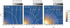 |
Fig. 1 Envelope of a growing planet at three different mass stages (left 30ME,
centre 100ME,
right 330ME). The azimuthally-averaged density-weighted mean velocity ( |

3.2 Rotation in the envelope and implications for satellite formation
As the planet grows in mass, the angular momentum distribution inside the envelope changes. This evolution can be seen in Fig. 1, where the white curves show the ratio of the specific angular momentum with respect to the pure Keplerian rotation in the midplane f = hz∕hKep, as measured around the polar axis in a frame co-moving with the planet, but not rotating around it1. Here,  is the angular momentum of gas in Keplerian rotation, expected to be approached when gas settles in a disc around a central potential. Around low-mass planets (≲ 30ME) we find that the angular momentum distribution is well explained by the circumstellar Keplerian shear penetrating deep into the envelope2 (Lambrechts & Lega 2017). Larger planets (≳ 30 ME), however, gain prograde angular momentum. However, the angular momentum increase is only moderate, because we do not see a clear signature of circumplanetary discs in our simulations. Only Jupiter-mass planets reveal a hint of a disc-like structure which shows strongly sub-Keplerian rotation. Possibly, this is related to a more 2D-like mass flow around larger mass planets (Ormel et al. 2015b).
In the context of the Solar System, the apparent lack of circumplanetary discs, at least around the lower mass planets in the ice giant mass-regime, argues against scenarios where regular satellites form in circumplanetary discs (Canup & Ward 2002). Therefore, the regular moons around Uranus and Neptune may rather be the product of late-formed tidal discs of solids that viscously relax and spawn satellites at the Roche radius (Crida & Charnoz 2012).
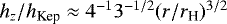
We note that for the 100ME planet the inner 50% of the Hill sphere is too warm to allow the condensation of ices, while for the Jupiter mass planet this region encompasses nearly the whole Hill sphere. Such elevated temperatures do not appear to be favourable to the formation of icy regular moons. Possibly, this implies that circumplanetary discs only appear late, when the circumstellar disc cools down and dissipates, which is a topic for further study. For now, we can make a crude order of magnitude analysis of the spin angular momentum stored in the bound interior, within r ≲ 0.3rH. We find a centrifugal radius of the bound envelope which is about  , where the reference value of f ≈ 0.2 at r = 0.3rH can be read from Fig. 1. Here, we assumed no angular momentum loss and ignoring pressure effects and viscous spreading. For comparison, the outermost regular satellite for each giant planet in the Solar System is situated between 10−3 rH (Proteus around Neptune) and 5.4 × 10⁻² rH (Iapetus around Saturn). Further contraction, without angular momentum loss, would imply exceeding break-up velocity. Therefore, it appears that giant planets need to shed their angular momentum efficiently, which may be possible through magnetic coupling between the planet and a circumplanetary disc (Batygin 2018).
3.3 Gas accretion
To a good approximation the interior envelope can be thought of as being in hydrostatic balance and in the process of slowly contracting, and thus accreting, over time. Indeed, the velocity field shown in the different panels of Fig. 1 reveals that the envelope interior to ≲0.3 rH is shielded from the mass flux through the outer envelope.
We computed the gas accretion rate by monitoring the increase in the envelope mass inside 0.3 rH, during 8 orbits (see Appendix A for more details). These measurements are represented by the red symbols in Fig. 2. In general we find good agreement with similar accretion rate measurements made using an SPH method (Ayliffe & Bate 2009). However, we do not find a turnover in accretion rate leading to decreasing accretion rates beyond 100ME. As can be seen in Fig. 2 (triangle symbols), we do find that our accretion rates increase gently when we refine simulations by reducing the smoothing length and increasing the resolution (a more detailed discussion can be found in Appendix A).
We verified that these measured accretion rates are consistent with the energy released by compressional heating in the interior envelope that is dominantly generated through gas settling in the gravitational potential, through the relationship  . Here L is the luminosity from compressional heating (obtained by integrating over the dominant compression term in the energy equation, − P ⋅∇u, with P the pressure and u the gas velocity) and rs is the smoothing length. This agreement is our first line of evidence for gas being accreted through quasi-static contraction of the inner envelope.
We also find that the scaling of the accretion rate with planetary mass can be approximately reproduced with our 1D evolution model (black dashed line in Fig. 2, see Appendix B for description of the model). We note here that matching the absolute values of 3D accretion rates with 1D rates is difficult, because of the various approximations made in the 1D and 3D calculations, which includes the approximate potential description in 3D. Therefore, in this work, we do not aim to directly link 1D and 3D models, as done in Lissauer et al. (2009); D’Angelo & Bodenheimer (2013). Instead, for now, we simply evolve planets in the toy model with an effective opacity of κeff = 0.01 cm2 g−1 at the radiative convective boundary. This parameter should thus not be thought of as a true opacity, but rather a free parameter that encapsulates our approximations and which effectively allows us to scale the growth rates as  . In this way, without aiming for precise quantitative agreement, we do reproduce the scaling relation of accretion rate with planetary mass. We find from our 3D simulations that the mass accretion rate scales approximately with the planetary mass as Ṁ ∝M1.5−2 (Fig. 2), in approximate agreement with our 1D toy model. Therefore, this supports that, to a good approximation, even high-mass planets accrete through quasi-static contraction and the accreting gas is never in dynamical free-fall.
In the low-mass regime, below 100ME, our 3D accretion rates appear to be also in crude agreement with previous detailed 1D model studies (Tajima & Nakagawa 1997; Ikoma et al. 2000). For example, Tajima & Nakagawa (1997) report accretion rates of the order of 10−4 ME yr−1 around a 30ME-planet. However, at larger planetary masses we see a divergence between our 3D accretion rates and those found in 1D studies such as those by Tajima & Nakagawa (1997) and Ikoma et al. (2000) that report a steeper scaling of the accretion rate with mass. However, a less steep dependency is found by Mordasini et al. (2012), as pointed out by Ida et al. (2018). The exact origin of this difference may be related to the treatment of the equation of state for the H/He-envelope, in the form of a variable adiabatic index prescription. In contrast, in our study, we have used for consistency a fixed adiabatic index (γ = 1.4) for both the 1D toy model and our 3D simulations. This choice for the fixed γ was motivated by our 3D simulations where, due to our limited central resolution, even the inner mass layers do not reach the conditions for ionisation and dissociation that require the variable γ approach (see also Appendix A). Further addressing this point would thus require even higher resolution studies.
An important caveat to this study is that we do not yet explore different disc conditions. We expect that lower gas surface densities and lower disc viscosities could reduce the supply of disc gas to the planet. Moreover, we have used here an opacity prescription where, in the low-temperature regime, opacities are dominated by the dust component. In this standard approach, μm-dust sizes and a dust-to-gas ratio of Z = 0.01 are assumed, which is consistent with the interstellar medium (Bell & Lin 1994). In reality, dust growth through sticking may deplete the small μ-sized grains (Brauer et al. 2008). The resulting smaller opacities would lead to larger gas accretion rates, as energy is more easily radiated away. Although we have attempted to use nominal disc parameters in this study, more work will be necessary to map out the influence of these parameters (Schulik et al. 2019). Another caveat is that this work does not make use of smoothing lengths below rs ∕rH = 0.1. Therefore we do not fully model the envelope interior to the smoothing length and this issue is discussed in more detail in Appendix A.
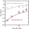 |
Fig. 2 Gas accretion rates as function of planetary mass. Red circles indicate mass accretion rates obtained from the hydrodynamical simulations, for each of the different planetary masses we probed. Grey squares represent the measured mass flux through the outer envelope, measured through the Hill sphere. Grey and red triangles correspond to results from our highest resolution runs (run100HR,run330HR). The black dashed curve shows the evolution of the mass accretion rate obtained with a simplified 1D model in order to capture the long-term evolution. The grey dashed line shows Eq. (2), where we included the turn-over around one Jupiter mass as in Tanigawa & Ikoma (2007). We found this expression corresponds well with the bulk mass flux through the envelope, but not with the gas accretion rate. |
3.3.1 Low-mass planets
Planets with masses below 100ME are relatively slow accretors, with rates as low as Ṁgas ≈ 2 × 10⁻⁵ ME yr−1 around 15ME planets. Interestingly, they also show the largest difference in the accretion rate versus the flux of gas that passes through the outer layers of the Hill sphere. We measure here the mass flux as the mass flux entering the Hill sphere, not the net flux difference between the mass flow moving in and out3 (Fig. 2). For the 15ME planet, the unsigned mass flux transiting the envelope is of the order of Ṁgas ≈ 10−1 ME yr−1, which is four orders of magnitude larger than the actual accretion rate.
We also find that the mass accretion rate (red symbols) and the transiting mass flux through the envelope (grey symbols) scale differently with respect to planetary mass, as can be seen in Fig. 2. Nevertheless, in the literature this mass flux throughthe envelope seems in some cases to have been interpreted as a gas accretion rate (D’Angelo et al. 2003; Machida et al. 2010; Tanigawa & Tanaka 2016). Indeed, we find that the mass flux through the envelope is well described by the expression
![\begin{align*} \dot M_{\textrm{flux}} \approx &\, 0.4 \times \left( \frac{M_{\textrm{p}}}{100\,\it M_{\textrm{E}}} \right)^{4/3} \left( \frac{r_{\textrm{p}}}{5\,\rm AU} \right)^{1/2}\nonumber\\[3pt] & \quad\ \ \times\left( \frac{H_{\textrm{p}}/r_{\textrm{p}}}{0.04} \right)^{-2} \left( \frac{\Sigma_{\textrm{g}}}{410\,\textrm{g\,cm}^{-2}} \right)^{4/3} \,\frac{M_{\textrm{E}}}\textrm{yr} \,,\end{align*}](/articles/aa/full_html/2019/10/aa34413-18/aa34413-18-eq8.png) (2)
(2)
which was previously reported as the accretion rate before gap opening (Tanigawa & Watanabe 2002). Here, Mp and rp are the mass and orbital radius of the planet. Σg is the gas surface density and Hp∕rp is the aspect ratio of the protoplanetary disc, measured at the location of the planet. The grey dashed line in Fig. 2shows Eq. (2), but also includes the gap formation induced turn-over around Jupiter mass as in Tanigawa & Ikoma (2007) and Tanigawa & Tanaka (2016).
Finally, we note that these high mass fluxes through the envelope do not appear to strongly quench gas accretion rates. This occurs because the cooling interior of the planet remains shielded from the advection of gas and a convective-radiative-advective three-layer envelope structure develops (Lambrechts & Lega 2017).
3.3.2 High-mass planets
Higher mass planets start carving a gap in the disc, as tidal and pressure torques overcome the viscous torque (Crida et al. 2006). However, this process does not halt the flow of gas through the outer atmosphere (Morbidelli et al. 2014). We find indeed that the mass flow rates through the envelope remain of the same order of magnitude and are comparable to the flux given in Eq. (2). At most, the decrease in the local gas surface density due to gap formation leads to the rate of mass flux through the envelope leveling off around planets larger than 200ME (Tanigawa & Ikoma 2007; Tanigawa & Tanaka 2016).
Gas accretion rates similarly appear not affected by gap formation. The accretion rates continue to grow with mass, as can be seen in Fig. 2, and follow the same trend as our 1D-model. Gas accretion rates become as high as 10−2 ME yr−1 around Jupiter mass planets. We nevertheless caution that further work is required to study gas accretion in the context of gap formation in low viscosity discs with long viscous equilibration timescales (Kanagawa et al. 2017).
Can a disc supply these high gas flow and gas accretion rates? Our simulations cannot address this question directly as they only cover an annulus of a gas disc during a short timescale. That being said, gas accretion rates onto solar-like stars can initially be as high as approximately 10−7 M⊙ yr−1, while decaying to about 10−9 M⊙ yr−1 near the end of the disc lifetime (Antoniucci et al. 2014; Manara et al. 2016; Hartmann et al. 2016). This would correspond to a global flow rate of gas through the disc of approximately 3.3 × 10⁻² to 3.3 × 10⁻⁴ ME yr−1. Therefore, in the first few Myr, discs can provide gas to accreting giant planets. Only gas giants that emerge near the end of the disc lifetime may see diminished gas accretion rates. However, even these giant planets would still be able to double their mass in about a Myr. That being said, the complicated interplay between gas accretion, gap formation and disc depletion warrants further study.
4 Implications
Observations of short-period giant exoplanets, that are larger than 15ME, show a wide and continuous range of envelope-to-core mass ratios, ranging from planets where the envelope mass barely exceeds the core mass, up to gas giants as large as about 4 Jupiter masses4. This is surprising given that planets larger than 15ME are susceptible to runaway gas accretion, if they form sufficiently early to spend more than approximately a Myr in the gas disc (Lambrechts & Lega 2017). Runaway gas accretion would only produce planets with high envelope-to-core mass ratios, contrary to these observations. Why some cores accrete thick envelopes, and others do not, is difficult to explain within our current theoretical understanding. We consider two cases, late and early formation.
Our study supports a scenario where giant planets reach the point of runaway gas accretion late in the approximately 3 Myr-lifetime of the protoplanetary disc. We find increasing gas accretion rates for planets of increasing mass, such that when they are joined in an evolutionary sequence they correspond to Jupiter growing to completion in 1 Myr, as illustrated in Fig. 3. Here, the black curve shows the time evolution of the runaway gas phase, obtained by integrating a least-squares fit of a power law to the measured accretion rates of our hydrodynamical simulations. We find  . We prefer this over piece-wise integration due to the sparse mass sampling. Given the previously discussed uncertainties in the accretion rates, the time obtained here for runaway gas accretion is only approximate. We find that the growth from 15 to 330ME would be completed in about 2 × 10⁵ yr. However, most of the time growing is spent when the planet is smaller than 15ME, as indicated by the 1D model (grey dashed curve). Therefore, mainly for illustrative purposes, we have shifted the black growth curve by ≈ 0.8 Myr to match the point where the 1D planet reached 30ME, but we note that this early contraction phase is sensitive to when solid accretion halted onto the planet and the final core mass (Lambrechts & Lega 2017). That being said, the short time-scale for runaway gas accretion we measure here would thus argue for scenario where giant planets like Jupiter emerged late in the disc lifetime, in order to explain their present day mass.
This late-formation view is possibly supported by the emerging populations of exoplanets detected through microlensing surveys (Suzuki et al. 2016). This technique probes exoplanets down to approximately Neptune mass, in orbits around the ice line of their host star, which is somewhat similar to the giant planets we consider in this work. Suzuki et al. (2016) report a single power law distribution for planet occurrence with respect to the planet-to-host-star mass q. They find that dN∕d log q ∝ qn, with n = −0.93 ± 0.1 holds well between Neptune to 10-Jupiter-mass planets. This also appears consistent with a recent analysis of the long-period transiting planet sample from Kepler (Herman et al. 2019). Thus, at least for this population of relatively wide-orbit planets, there appears to be no signature of a natural mass where accretion comes to a halt (which would translate in a sharp increase in the number of planets at that mass, Suzuki et al. 2018). Instead, the steep slope in occurrence rates seems more consistent with continued mass growth up until gas is removed from the protopanetary disc (a process independent of the planet mass). In fact, the slope of the mass distribution is a measure of the scaling of the gas accretion rate with mass, assuming a steady state distribution. Because  , it appears that giant planets grow approximately along Ṁ ∝ M−n+1 ∝ M1.9. Encouragingly, the observed mass accretion scaling appears to be consistent with the mass scaling we find numerically where Ṁ ∝ M1.5−2 (Fig. 2) and a least-squares fit gives Ṁ ∝ M1.9.
Alternatively, one can hypothesise runaway gas accretion occurred early in the evolution of the disc. Planetary cores could emerge within a Myr timescale in a pebble accretion scenario (Lambrechts & Johansen 2012, 2014; Bitsch et al. 2015). Such early core formation has been proposed for Jupiter in order to separate the inner and outer Solar System into two distinct isotopic reservoirs after only about 1 Myr of disc evolution (Kruijer et al. 2017). However, the fast appearance of giant planets is problematic for two reasons. Firstly, given the accretion rates we report, one needs to invoke an as of yet unknown physical mechanism to limit gas accretion onto the planet for potentially several Myr before the disc dissipates. Secondly, even if accretion could be halted, early-formed gas giants would migrate rapidly through discs (Bitsch et al. 2015), because of type-2 migration (Lin & Papaloizou 1986, but see also Dürmann & Kley 2017; Kanagawa et al. 2018 and Robert et al. 2018).
In summary, this work argues gas giant reached the point of runaway growth late in the disc lifetime, possibly due to slow pre-runaway gas accretion or the relatively late formation of planetary cores. However, more work will be necessary to understand the physical mechanisms behind the final masses, and orbital locations, of giant planets. A promising avenue for future work could be the study of planets in stratified low-viscosity discs where accretion and migration may be slower.
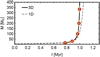 |
Fig. 3 Evolution of the planetary mass as function of time, based on the snapshot accretion rates of our hydrodynamical simulations (black curve). Red circles mark the masses where hydrodynamical simulations were performed. The measured accretion rate of each simulation is indicated by the orange slope segment. Growth from a 15ME-planet to a Jupiter-mass planet is completed in about 2 × 10⁵ yr. The grey dashed curve represents the 1D model, illustrating a significant fraction of envelope growth may be spend at low envelope masses. |
5 Conclusions
In this paper, we have numerically investigated how giant planets accrete their gaseous envelopes. For planets between 15 ME and 1 MJ in mass, we have measured that gas accretion proceeds through quasi-static contraction of a nearly hydrostatic envelope that is located within the inner ~30% of the Hill radius.
The accretion rate of material onto the inner bounded envelope is between 2 and 4 orders of magnitude lower than mass flux of gas into the Hill sphere. Moreover, the effective accretion rate shows a different scaling relation with planetary mass compared to the mass flux through the Hill sphere. Therefore, the complex 3D gas flow in the outer envelope is limited tothe advection of gas in and out of the Hill sphere, and unrelated to the gas accretion rate onto the planet. We do not identify the presence of a circumplanetary disc around accreting planets smaller than about 100ME in mass.
Our model suggests that, after the emergence of an approximately 15ME-planet, the formation of a Jupiter-mass planet can occur within approximately 2 × 10⁵ yr at 5 AU, assuming an ISM-like opacity. These growth rates are however dependent on the opacity, viscosity and gas surface density, and these dependencies need further exploration. Moreover, our study makes use of a smoothing parameter that regulates how centrally condensed the gravitational potential is. Therefore our results are focussed on the description of the envelope outside of approximately 0.1rH. Further high-resolution 3D simulations with radiative transfer, that include high-temperature changes in the equation of state, and ideally the inclusion of self-gravity, will be needed to explore the role of the deep envelope interior within 0.1rH. An interesting prospect is that such work would allow probing the convective interior and characterise the radiative-convective boundary, an important transition that would facilitate the comparison to 1D models (Ikoma et al. 2000; Piso & Youdin 2014).
Finally, our radiative hydrodynamical simulations do not reveal any thermally induced processes that can strongly reduce the accretion of massive gas envelopes on Myr timescales. In the absence of other processes that can slow down accretion, this implies that the masses of the giant planets in the Solar system are most naturally explained because they formed in a limited gas reservoir, most likely due to forming late in the lifetime of the protoplanetary disc.
Acknowledgements
M.L. likes to thank Bertram Bitsch, Matthäus Schulik, Anders Johansen, and Yuri Fujii for stimulating discussions. The authors are grateful for the constructive feedback by an anonymous referee. M.L., E.L., A.C., and A.M. are thankful to ANR for supporting the MOJO project (ANR-13-BS05-0003-01). R.P.N. acknowledges support from the STFC grants STP0005921 and STM0012021. This work was performed using HPC resources from GENCI [IDRIS] (Grant 2017/2018, [i2016047233]) and Mesocentre SIGAMM, hosted by the Observatoire de la Côte d’Azur.
Appendix A Numerics
Resolution
We have tested our results against changes in resolution and the choice of the smoothing length of the potential. This is illustrated in Fig. A.1. Here, the mass in an envelope shell is plotted as function of time for run100 (black curves). After relaxing the potential over an orbital period, the interior envelope, within r ≲ 0.3rH, starts to contract and accrete mass. We find then, similar to Lambrechts & Lega (2017), that the luminosity of the planet reaches an approximate steady state balance after the adjustment the changing potential. As shown in Fig. A.1, the outer envelope shells do not participate significantly in the accumulation of mass. Because mass growth occurs in the centre, it is necessary tomodel the interior with sufficient resolution.
For a fixed smoothing length, we empirically identified that when using above 8 cells per smoothing length we obtain convergent behaviour in the interior structure and accretion rate. Indeed, a simulation with twice the resolution gives similar accretion rates (orange curves, labelled HRS02). Conversely, in simulations where a too low resolution per smoothing length is introduced, the balance between gravity and pressure support can get destabilised. This is illustrated with a test run indicated by the grey curves (labelled LRS01) in Fig. A.1. Therefore, our standard practice when halving the smoothing length is to double the resolution, we term this procedure refinement.
As mentioned in Sect. 3.3, accretion rates increase moderately when we refine the simulations. This can also be seen in Fig. A.1, where run100 (black curve) can be compared with run100HR (red curve). We thus find slightly higher accretion rates with increasing refinement. This physical effect occurs because reducing the smoothing length effectively opens up a new interior region of the planet. A refinement by a factor of 2 between run100 and run100HR resulted in an increase of the mass accretion rate by a factor of about 1.5. Therefore, further reductions of the smoothing length could increase the accretion rate more, but high resolution studies indicate that little envelope contraction occurs in the strongly pressure-supported central envelope inside of 0.1rH (Szulágyi et al. 2016). This is also supported by the approximate agreement in measured accretion rates for 100ME-planets between our work and the SPH results of Ayliffe & Bate (2009) that use rs ∕rH < 0.01. Nevertheless, future studies aimed at resolving the deep interior will also need to address temperature dependent changes of the equations of state (further discussed below, see also Szulágyi et al. 2016) and should strive for a more realistic description of the gravitational potential by including selfgravity. Taken together, this does indicate that our study is limited to characterising accretion of envelope down to ≈ 0.1rH and further work is required to reveal the contraction of the deep interior, but for now, such higher resolution studies with rs ∕rH < 0.1 are currently numerically unfeasible for our model setup. We further note that deepening the gravitational potential, in principle down to the core surface, would also require longer envelope equilibration times exceeding 10 orbital timescales (Fig. A.1), which would further increase the numerical cost.
In our simulations we note a tendency for the accretion rate to start to decrease on long timescales (≳ 10 P). This is an artefact of our snapshot approach, where we do not take into account the effect of the accreted mass on the gravitational potential, which already starts to exceeds the 1% of the potential mass after 10 orbits for our Saturn-mass case. As a result, we pragmatically constrain our measurements of the accretion rates to be made within 10 orbits.
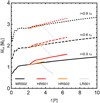 |
Fig. A.1 Envelope shell mass as function of time, interior to 0.3, 0.6, 0.9rH for the Saturn-mass case. Black curves correspond to run100, labelled as MRS02 (medium resolution, smoothing length rs ∕rH = 0.2). The smoothing length is relaxed to its final value over one orbit, corresponding to the initial increase in envelope mass. Further gas accretion is the result of the physical cooling of the envelope. Increasing the resolution even further does not change the accretion rate, as indicated by the orange curve (labelled HRS02). A refined simulation with twice the resolution and half the smoothing length (rs ∕rH = 0.1, run100HR) is shown in red. The grey curves represent a test simulation with factor 2 smaller smoothing length, but without the increase in resolution, which results in an unstable envelope. |
Equation of state
We verified that in our current simulations temperatures and densities are such that our ideal gas equation of state is not violated. For our Jupiter-mass simulation, temperatures in the most interior shell reach T = 1500 K and densities of ρ = 7.7 × 10⁻⁹ g cm−3. Therefore we do not yet reach the conditions where H/He ionisation starts playing a significant role (Piso et al. 2015; Popovas & Jørgensen 2016). However, future work making use of even more reduced smoothing lengths will probe more interior regions and will thus also require a more complete equation of state.
Appendix B 1D toy model
We make use of a simple 1D toy model to calculate the mass growth of an envelope. It assumes that the growth in atmospheric mass is the result of the competition between the gravitational contraction of the envelope and how efficiently the planet transports this heat release. In practice, we construct a cooling sequence. Subsequent stages of the envelope increase in mass, but see their total energy budget decrease due to release of heat, corresponding to a luminosity:
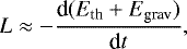 (B.1)
(B.1)
where Eth and Egrav are, respectively, the integrated thermal and gravitational energy stored in the envelope.
In order to time evolve the envelope, we perform an iterative procedure, where we require the energy loss during a timestep to be consistent with energy difference between subsequent envelope structures, which are assumed to be in hydrostatic equilibrium. This is a common technique used in 1D-models (Bodenheimer & Pollack 1986; Pollack et al. 1996; Ikoma et al. 2000; Papaloizou & Nelson 2005; Mordasini et al. 2012; Piso & Youdin 2014; Lee et al. 2014; Coleman et al. 2017). In practice, we first calculate the envelope structure for a given envelope mass. We then time step and predict the subsequent envelope mass. The chosen envelope mass fixes the envelope structure and the energy budget. We then perform a convergence step, where we vary the envelope mass until we reach energy balance. An in detail prescription of this numerical approach will be given in Lambrechts & Johansen (in prep.).
This procedure is based on several simplifying assumptions, in order to efficiently calculate the long-term evolution of the planet. We assume spherical symmetry. Moreover, we assume that envelopes are in perfect hydrostatic equilibrium, from the core to the outer boundary, here set to be the Hill sphere. At this outer boundary the envelope connects to the unperturbed nebular temperature T and density ρ. The outer radiative region is assumed to be isothermal. Additionally, the opacity at the radiative convective boundary is held fixed over time. Finally, the inner convective interior is approximated as a self-gravitating polytrope with adiabatic index γ = 1.4, which is solved for through the Lane–Emden equation. In conclusion, in the toy model we assume that planets evolve at all times, and for all masses, through quasi-static contraction. This allows us to use the total energy budget of the planet to evolve the planet forward in time, without the need for numerically expensive radiative transfer, but at the cost of a priori difficult to motivate assumptions on the structure and evolution of the envelope.
References
- Antoniucci, S., García López, R., Nisini, B., et al. 2014, A&A, 572, A62 [NASA ADS] [CrossRef] [EDP Sciences] [Google Scholar]
- Ayliffe, B. A., & Bate, M. R. 2009, MNRAS, 393, 49 [NASA ADS] [CrossRef] [Google Scholar]
- Batygin, K. 2018, AJ, 155, 178 [NASA ADS] [CrossRef] [Google Scholar]
- Bell, K. R., & Lin, D. N. C. 1994, ApJ, 427, 987 [NASA ADS] [CrossRef] [Google Scholar]
- Bitsch, B., Crida, A., Morbidelli, A., Kley, W., & Dobbs-Dixon, I. 2013, A&A, 549, A124 [NASA ADS] [CrossRef] [EDP Sciences] [Google Scholar]
- Bitsch, B., Lambrechts, M., & Johansen, A. 2015, A&A, 582, A112 [NASA ADS] [CrossRef] [EDP Sciences] [Google Scholar]
- Bitsch, B., Morbidelli, A., Johansen, A., et al. 2018, A&A, 612, A30 [NASA ADS] [CrossRef] [EDP Sciences] [Google Scholar]
- Bodenheimer, P., & Pollack, J. B. 1986, Icarus, 67, 391 [NASA ADS] [CrossRef] [Google Scholar]
- Brauer, F., Dullemond, C. P., & Henning, T. 2008, A&A, 480, 859 [NASA ADS] [CrossRef] [EDP Sciences] [Google Scholar]
- Bryden, G., Chen, X., Lin, D. N. C., Nelson, R. P., & Papaloizou, J. C. B. 1999, ApJ, 514, 344 [NASA ADS] [CrossRef] [Google Scholar]
- Canup, R. M., & Ward, W. R. 2002, AJ, 124, 3404 [NASA ADS] [CrossRef] [Google Scholar]
- Cimerman, N. P., Kuiper, R., & Ormel, C. W. 2017, MNRAS, 471, 4662 [NASA ADS] [CrossRef] [Google Scholar]
- Coleman, G. A. L., Papaloizou, J. C. B., & Nelson, R. P. 2017, MNRAS, 470, 3206 [NASA ADS] [CrossRef] [Google Scholar]
- Crida, A., & Charnoz, S. 2012, Science, 338, 1196 [NASA ADS] [CrossRef] [Google Scholar]
- Crida, A., Morbidelli, A., & Masset, F. 2006, Icarus, 181, 587 [Google Scholar]
- D’Angelo, G., & Bodenheimer, P. 2013, ApJ, 778, 77 [NASA ADS] [CrossRef] [Google Scholar]
- D’Angelo, G., Kley, W., & Henning, T. 2003, ApJ, 586, 540 [NASA ADS] [CrossRef] [Google Scholar]
- de Val-Borro, M., Edgar, R. G., Artymowicz, P., et al. 2006, MNRAS, 370, 529 [NASA ADS] [CrossRef] [Google Scholar]
- Dürmann, C., & Kley, W. 2017, A&A, 598, A80 [NASA ADS] [CrossRef] [EDP Sciences] [Google Scholar]
- Fung, J., Artymowicz, P., & Wu, Y. 2015, ApJ, 811, 101 [NASA ADS] [CrossRef] [Google Scholar]
- Gressel, O., Nelson, R. P., Turner, N. J., & Ziegler, U. 2013, ApJ, 779, 59 [NASA ADS] [CrossRef] [Google Scholar]
- Hartmann, L., Herczeg, G., & Calvet, N. 2016, ARA&A, 54, 135 [NASA ADS] [CrossRef] [Google Scholar]
- Herman, M. K., Zhu, W., & Wu, Y. 2019, AJ, 157, 248 [NASA ADS] [CrossRef] [Google Scholar]
- Ida, S., Tanaka, H., Johansen, A., Kanagawa, K. D., & Tanigawa, T. 2018, ApJ, 864, 77 [NASA ADS] [CrossRef] [Google Scholar]
- Ikoma, M., Nakazawa, K., & Emori, H. 2000, ApJ, 537, 1013 [NASA ADS] [CrossRef] [Google Scholar]
- Kanagawa, K. D., Tanaka, H., Muto, T., & Tanigawa, T. 2017, PASJ, 69, 97 [Google Scholar]
- Kanagawa, K. D., Tanaka, H., & Szuszkiewicz, E. 2018, ApJ, 861, 140 [NASA ADS] [CrossRef] [Google Scholar]
- Klahr, H., & Kley, W. 2006, A&A, 445, 747 [NASA ADS] [CrossRef] [EDP Sciences] [Google Scholar]
- Kley, W. 1999, MNRAS, 303, 696 [NASA ADS] [CrossRef] [Google Scholar]
- Kley, W., Bitsch, B., & Klahr, H. 2009, A&A, 506, 971 [NASA ADS] [CrossRef] [EDP Sciences] [Google Scholar]
- Kokubo, E., & Ida, S. 1998, Icarus, 131, 171 [NASA ADS] [CrossRef] [Google Scholar]
- Kruijer, T. S., Burkhardt, C., Budde, G., & Kleine, T. 2017, Proc. Natl. Acad. Sci., 114, 6712 [NASA ADS] [Google Scholar]
- Kurokawa, H.,& Tanigawa, T. 2018, MNRAS, 479, 635 [NASA ADS] [CrossRef] [Google Scholar]
- Lambrechts, M., & Johansen, A. 2012, A&A, 544, A32 [Google Scholar]
- Lambrechts, M., & Johansen, A. 2014, A&A, 572, A107 [NASA ADS] [CrossRef] [EDP Sciences] [Google Scholar]
- Lambrechts, M., & Lega, E. 2017, A&A, 606, A146 [NASA ADS] [CrossRef] [EDP Sciences] [Google Scholar]
- Lambrechts, M., Johansen, A., & Morbidelli, A. 2014, A&A, 572, A35 [NASA ADS] [CrossRef] [EDP Sciences] [Google Scholar]
- Lee, E. J., Chiang, E., & Ormel, C. W. 2014, ApJ, 797, 95 [NASA ADS] [CrossRef] [Google Scholar]
- Lega, E., Crida, A., Bitsch, B., & Morbidelli, A. 2014, MNRAS, 440, 683 [NASA ADS] [CrossRef] [Google Scholar]
- Lega, E., Morbidelli, A., Bitsch, B., Crida, A., & Szulágyi, J. 2015, MNRAS, 452, 1717 [NASA ADS] [CrossRef] [Google Scholar]
- Levermore, C. D., & Pomraning, G. C. 1981, ApJ, 248, 321 [NASA ADS] [CrossRef] [Google Scholar]
- Lin, D. N. C., & Papaloizou, J. 1986, ApJ, 309, 846 [NASA ADS] [CrossRef] [Google Scholar]
- Lissauer, J. J., Hubickyj, O., D’Angelo, G., & Bodenheimer, P. 2009, Icarus, 199, 338 [NASA ADS] [CrossRef] [Google Scholar]
- Lubow, S. H., Seibert, M., & Artymowicz, P. 1999, ApJ, 526, 1001 [NASA ADS] [CrossRef] [Google Scholar]
- Machida, M. N., Kokubo, E., Inutsuka, S.-I., & Matsumoto, T. 2010, MNRAS, 405, 1227 [NASA ADS] [Google Scholar]
- Manara, C. F., Fedele, D., Herczeg, G. J., & Teixeira, P. S. 2016, A&A, 585, A136 [NASA ADS] [CrossRef] [EDP Sciences] [Google Scholar]
- Masset, F. 2000, A&AS, 141, 165 [NASA ADS] [CrossRef] [EDP Sciences] [Google Scholar]
- Mizuno, H. 1980, Prog. Theor. Phys., 64, 544 [Google Scholar]
- Morbidelli, A., & Nesvorny, D. 2012, A&A, 546, A18 [NASA ADS] [CrossRef] [EDP Sciences] [Google Scholar]
- Mordasini, C., Alibert, Y., Klahr, H., & Henning, T. 2012, A&A, 547, A111 [NASA ADS] [CrossRef] [EDP Sciences] [Google Scholar]
- Morbidelli, A., Szulágyi, J., Crida, A., et al. 2014, Icarus, 232, 266 [NASA ADS] [CrossRef] [Google Scholar]
- Ormel, C. W., Shi, J.-M., & Kuiper, R. 2015a, MNRAS, 447, 3512 [NASA ADS] [CrossRef] [Google Scholar]
- Ormel, C. W., Kuiper, R., & Shi, J.-M. 2015b, MNRAS, 446, 1026 [NASA ADS] [CrossRef] [Google Scholar]
- Papaloizou, J. C. B., & Nelson, R. P. 2005, A&A, 433, 247 [NASA ADS] [CrossRef] [EDP Sciences] [Google Scholar]
- Piso, A.-M. A., & Youdin, A. N. 2014, ApJ, 786, 21 [NASA ADS] [CrossRef] [Google Scholar]
- Piso, A.-M. A., Youdin, A. N., & Murray-Clay, R. A. 2015, ApJ, 800, 82 [NASA ADS] [CrossRef] [Google Scholar]
- Pollack, J. B., Hubickyj, O., Bodenheimer, P., et al. 1996, Icarus, 124, 62 [NASA ADS] [CrossRef] [Google Scholar]
- Popovas, A., & Jørgensen, U. G. 2016, A&A, 595, A130 [NASA ADS] [CrossRef] [EDP Sciences] [Google Scholar]
- Popovas, A., Nordlund, Å., Ramsey, J. P., & Ormel, C. W. 2018, MNRAS, 479, 5136 [NASA ADS] [CrossRef] [Google Scholar]
- Robert, C. M. T., Crida, A., Lega, E., Méheut, H., & Morbidelli, A. 2018, A&A, 617, A98 [NASA ADS] [CrossRef] [EDP Sciences] [Google Scholar]
- Santos, N. C., Adibekyan, V., Figueira, P., et al. 2017, A&A, 603, A30 [NASA ADS] [CrossRef] [EDP Sciences] [Google Scholar]
- Schulik, M., Johansen, A., Bitsch, B., & Lega, E. 2019, A&A, accepted [Google Scholar]
- Stevenson, D. J. 1982, Planet. Space Sci., 30, 755 [NASA ADS] [CrossRef] [Google Scholar]
- Suzuki, D., Bennett, D. P., Sumi, T., et al. 2016, ApJ, 833, 145 [NASA ADS] [CrossRef] [Google Scholar]
- Suzuki, D., Bennett, D. P., Ida, S., et al. 2018, ApJ, 869, L34 [NASA ADS] [CrossRef] [Google Scholar]
- Szulágyi, J., Morbidelli, A., Crida, A., & Masset, F. 2014, ApJ, 782, 65 [NASA ADS] [CrossRef] [Google Scholar]
- Szulágyi, J., Masset, F., Lega, E., et al. 2016, MNRAS, 460, 2853 [NASA ADS] [CrossRef] [Google Scholar]
- Tajima, N., & Nakagawa, Y. 1997, Icarus, 126, 282 [NASA ADS] [CrossRef] [Google Scholar]
- Tanigawa, T., & Ikoma, M. 2007, ApJ, 667, 557 [NASA ADS] [CrossRef] [Google Scholar]
- Tanigawa, T., & Tanaka, H. 2016, ApJ, 823, 48 [NASA ADS] [CrossRef] [Google Scholar]
- Tanigawa, T., & Watanabe, S.-i. 2002, ApJ, 580, 506 [NASA ADS] [CrossRef] [Google Scholar]
- Tanigawa, T., Ohtsuki, K., & Machida, M. N. 2012, ApJ, 747, 47 [NASA ADS] [CrossRef] [Google Scholar]
The shown specific angular momentum linert in the inertial frame around the planetary polar axis is given by linert = lrot + ΩKr2, with ΩK the Keplerian frequency of the planet around the sun and lrot the specific angular momentum measured in the frame centred on the planet, with one axis along the direction to the star.
In the non-rotating frame circumstellar Keplerian shear would give
 (Lambrechts & Lega 2017).
The gas accretion rate is Ṁenv = −∫VF ⋅ndS, with n the unit vector on surface element dS and V the measurement volume, here taken to be a sphere around the approximately bound interior with radius r = 0.3 rH. The mass flux through the envelope we take to be Ṁflux = −∫V(F ⋅n)|F⋅n<0dS, with the volume V now given by the Hill sphere, in other words we only consider the mass flowing into the volume.
The occurrence rates of larger stellar companions do not longer increase with stellar metallicity and therefore likely no longer trace planets formed in the core accretion scenario (Santos et al. 2017).
All Tables
All Figures
|
Fig. 1 Envelope of a growing planet at three different mass stages (left 30ME,
centre 100ME,
right 330ME). The azimuthally-averaged density-weighted mean velocity ( |
| In the text | |
|
Fig. 2 Gas accretion rates as function of planetary mass. Red circles indicate mass accretion rates obtained from the hydrodynamical simulations, for each of the different planetary masses we probed. Grey squares represent the measured mass flux through the outer envelope, measured through the Hill sphere. Grey and red triangles correspond to results from our highest resolution runs (run100HR,run330HR). The black dashed curve shows the evolution of the mass accretion rate obtained with a simplified 1D model in order to capture the long-term evolution. The grey dashed line shows Eq. (2), where we included the turn-over around one Jupiter mass as in Tanigawa & Ikoma (2007). We found this expression corresponds well with the bulk mass flux through the envelope, but not with the gas accretion rate. |
| In the text | |
|
Fig. 3 Evolution of the planetary mass as function of time, based on the snapshot accretion rates of our hydrodynamical simulations (black curve). Red circles mark the masses where hydrodynamical simulations were performed. The measured accretion rate of each simulation is indicated by the orange slope segment. Growth from a 15ME-planet to a Jupiter-mass planet is completed in about 2 × 10⁵ yr. The grey dashed curve represents the 1D model, illustrating a significant fraction of envelope growth may be spend at low envelope masses. |
| In the text | |
|
Fig. A.1 Envelope shell mass as function of time, interior to 0.3, 0.6, 0.9rH for the Saturn-mass case. Black curves correspond to run100, labelled as MRS02 (medium resolution, smoothing length rs ∕rH = 0.2). The smoothing length is relaxed to its final value over one orbit, corresponding to the initial increase in envelope mass. Further gas accretion is the result of the physical cooling of the envelope. Increasing the resolution even further does not change the accretion rate, as indicated by the orange curve (labelled HRS02). A refined simulation with twice the resolution and half the smoothing length (rs ∕rH = 0.1, run100HR) is shown in red. The grey curves represent a test simulation with factor 2 smaller smoothing length, but without the increase in resolution, which results in an unstable envelope. |
| In the text | |
Current usage metrics show cumulative count of Article Views (full-text article views including HTML views, PDF and ePub downloads, according to the available data) and Abstracts Views on Vision4Press platform.
Data correspond to usage on the plateform after 2015. The current usage metrics is available 48-96 hours after online publication and is updated daily on week days.
Initial download of the metrics may take a while.