| Issue |
A&A
Volume 630, October 2019
Rosetta mission full comet phase results
|
|
|---|---|---|
| Article Number | A10 | |
| Number of page(s) | 8 | |
| Section | Planets and planetary systems | |
| DOI | https://doi.org/10.1051/0004-6361/201834127 | |
| Published online | 20 September 2019 | |
Generation of photoclinometric DTMs for application to transient changes on the surface of comet 67P/Churyumov-Gerasimenko
1
Astronomy Department, Cornell University,
Ithaca
NY, USA
e-mail: This email address is being protected from spambots. You need JavaScript enabled to view it.
2
Cornell Center for Astrophysics and Planetary Science, Cornell University,
Ithaca NY, USA
3
US Geological Survey, Astrogeology Division,
Flagstaff AZ, USA
4
Deutsches Zentrum für Luft-und Raumfahrt (DLR), Institut für Planetenforschung,
Rutherfordstraße 2,
Berlin, Germany
Received:
30
August
2018
Accepted:
28
February
2019
Abstract
Context. The wide spatial and temporal coverage of 67P/Churyumov-Gerasimenko (67P) by the Rosetta mission has revealed a surface created by scattered large-scale changes and numerous small-scale changes. The many small-scale changes are of particular interest because they are unexpected and ubiquitous. As their topographic relief is often smaller than one meter, which is below the resolution of any shape models, we need higher resolution topography to analyze them properly.
Aims. We describe a photoclinometry method that is able to retrieve surface elevations for a single OSIRIS image of the surface of 67P. With this method, we can provide accurate measures, along with error estimates, of the centimeter-scale topography of observed transient changes.
Methods. Photoclinometry, or shape-from-shading, estimates heights by examining the light reflection of the surface as dictated by a photometric model under a specified set of viewing geometries. Assuming a standard photometric model for 67P, we can recreate the shading of a surface under specified viewing geometries. The output is a high-resolution height map that matches the original image pixel by pixel. We then provide estimates of the error in the retrieved heights and ensure that our method is valid with a series of checks.
Results. We generate digital terrain models (DTMs) with a vertical resolution comparable to or smaller than the pixel scale. This allows us to accurately measure changes in the surface topography on centimeter scales. We find that most changes within the smooth terrains involve the transport or removal of material thinner than one meter.
Key words: comets: individual: 67P/Churyumov-Gerasimenko / techniques: image processing / methods: data analysis
© ESO 2019
1 Introduction
Spacecraft observations of cometary nuclei have just recently revealed processes at the comet surfaces with resolutions at the scale over which changes occur. Ground-based observations of comets have been unable to resolve the surface of a comet nucleus, while previous spacecraft missions involved only flybys at relatively large distances. The returned images were obtained at distances of ~180−600 km away from the nuclei (Keller et al. 1986; Veverka et al. 2013) and indicated complex and diverse landscapes. Furthermore, while comets are clearly active bodies, the only change in a nucleus observed before Rosetta was reported from 9P/Tempel 1 between the flybys of the Deep Impact and Stardust-NEXT missions. Near a retreating scarp of smooth material, several round depressions expanded and merged during one orbit (Veverka et al. 2013; Thomas et al. 2013).
ESA’s Rosetta mission to comet 67P/Churyumov-Gerasimenko (hereafter 67P) was able to provide unique and unprecedented views of the surface of 67P both in terms of spatial resolution and temporal coverage of the OSIRIS cameras (Keller et al. 2007). For more than 2.5 yr, Rosetta provided images that revealed centimeter-scale surface features (Sierks et al. 2015) and provided detailed observations of numerous surface changes (Groussin et al. 2015; El-Maarry et al. 2017; Hu et al. 2017). By studying these changes, we can better understand the processes governing the evolution of 67P, and they also provide valuable information that can be used for future exploration and sampling of their surfaces (e.g., NASA’s CAESAR mission).
Rosetta data have shown that surface changes can be categorized into two main categories: large-scale changes of the bulk nucleus, and small-scale changes of the smooth terrain material (El-Maarry et al. 2017). Large-scale changes to the nucleus were expected to occur during perihelion because debris lined most cliff margins, which is suggestive of mass wasting (Vincent et al. 2015). Furthermore, large-scale pits dominated the landscape of the northern hemisphere (Vincent et al. 2015), suggesting collapse of this material and progressive flattening of the terrains over multiple perihelion passages (Birch et al. 2017). Very few collapses of cliff margins were observed, suggesting that such large-scale changes either occurred in the past or that these changes occur over longer timescales. Small-scale changes in the smooth terrains, on the spatial order of ~10 m, were the dominant type of surface change (Vincent & Team 2018). These include features such as ripples in the Hapi region (Jia et al. 2017), retreat of scarps within smooth terrains (El-Maarry et al. 2017), formation of depressions (Groussin et al. 2015; Hu et al. 2017), and reorganization of material by dust deposition (Vincent & Team 2018). These numerous and diverse sets of observations thus raise questions regarding the physical nature of these changes, the processes, timescales, and orbital conditions that allow their formation, as well as their evolution and relations, if any, to each other.
To answer these questions, quantitative analyses that are able to measure the topographic form of the changes are required. However, these features are quite small, and so they are not captured in the large-scale shape models. Instead, we have adapted a well-vetted photoclinometry algorithm (Kirk et al. 2003) that allows for precise measures of the topography for a single Rosetta OSIRIS Narrow Angle Camera (NAC) image. The power of photoclinometry is that we can generate digital terrain models (DTMs) of a surface at the pixel scale using only a single image, which allows us to quantify changes in the surface topography from image to image.
In Sect. 2 we provide an overview of the process we used to apply the photoclinometric algorithms (Kirk et al. 2003) to Rosetta OSIRIS images. In Sect. 3 we demonstrate that this method consistently reproduces a given landform for multiple images of the same scene, even at different viewing geometries. We further analyze these scenes to provide quantitative estimates of the DTM precision and repeatability. In Sect. 4 we apply this method to numerous known changes in the smooth terrains to quantify their topographic form.
2 Photoclinometry methodology
Photoclinometry, or shape-from-shading, estimates heights by quantifying the reflected light from the surface as dictated by a photometricmodel, under a specified set of viewing geometries. We use photoclinometry because it requires only one image to operate, creates DTMs at the same scale as the original image, and has a history of reliable usage for other planetary surfaces, including a previous study of the surface of 67P (Birch et al. 2017). Stereophotogrammetry (SPG) and/or stereophotoclinometry (SPC) are not applicable in this case because it is difficult to acquire multiple images of the same transient features before and after their formation that are of the same quality, but with different lighting conditions. For an analysis of jets from the surface, stereo is possible with the assumption that the jet occurs at the same place, using images from multiple orbits of 67P (about one day apart) (Shi et al. 2018). Thus, in many cases where changes occur, the required matching image pairs are not available in the OSIRIS dataset because between orbits the feature, by definition, will have moved.
Photoclinometry requires knowledge of exact viewing geometries to accurately produce a DTM. We used the header information and routines in the Navigation and Ancillary Information Facility (NAIF) SPICE (Acton 1996) toolkit to calculate the viewing geometry for each pixel in any given OSIRIS NAC image. Because the body of 67P is irregular, we accomplished this by using thealpha-test Digital Shape Kernel (DSK) toolkit along with the SHAP4S shape model of 67P, a 4 million plate shape model created using SPG (Preusker et al. 2015). The SPG shape model was solely used as an initial basis for later iterations (Fig. 1). Furthermore, the exact choice of shape model does not affect our results (Sect. 3.2) so long as the long-wavelength topography between individual shape models remains consistent.
Together, this allows us to calculate the intersections of pixel vectors and the surface of 67P. Combined with the location of the Sun, thenormal vector of each plate of the shape model, and the location of the OSIRIS NAC, we are able to derive unique viewing geometries for every pixel (Fig. 1b). Because photometric contrast depends strongly on the incidence and phase angles, this process also finds the correct orientation of the surface and enables calibration of the surface brightness and contrast for each individual image.
For each image, based on the viewing geometry, we used the Hapke photometric function (Hapke 1981), along with parameters describing the phase function from Fornasier et al. (2015), to fit a Lunar-Lambert function (see McEwen 1991, Eq. (5)) for use in the photoclinometry. We did this by finding the mean ground plane of the surface and creating an isotropic Gaussian distribution of slopes relative to that plane. These slopes were then used to calculate a limb-darkening parameter and an overall brightness for the Lunar-Lambert function so that it best fits the Hapke function with parameters from Fornasier et al. (2015). While the limb-darkening parameter can now be used for the photoclinometry, the overall brightness cannot, as it describes the surface property of the comet instead of the reflectivity of the surface under the conditions of the specific image. To find the reflectance, or albedo, of an interested region, we created a rough, simulated image of the region (Fig. 2b) using the shape model terrain as an input (Fig. 1a). By dividing the original image by the simulated image, we were able to eliminate changes in brightness due to viewing geometries, leaving an approximate albedo map of the specific region in this image (Fig. 2c). We then used the average albedo across the region for photoclinometry (Fig. 2d).
We then assumed that the photometric model and surface properties were constant throughout our region of interest, which allowed us to recreate the shading of a surface under specified viewing geometries. Using the SHAP4S shape model surface as an initial estimate of the DTM (Fig. 1c), we iteratively adjusted DTM heights to maximize agreement between the shading of the DTM and the acquired image (Kirk et al. 2003, Fig. 3). Because this methodconverges local features faster than large-scale features, the use of the shape model surface as an initial estimate allowed recreating pixel scale details while retaining the large-scale topography of the shape model.
The output was a high-resolution height map that matches the original image pixel by pixel (Fig.1d). Whereas the original shape model only showed the long-wavelength topography, such as cliffs or broad basins, the DTMs we produced clearly showthe small-scale features, such as boulders and small scarps within the smooth terrains. Because a given DTM covers only a smallarea, the height errors do not accumulate such that they distort the overall shape of the surface (Sect. 3.1).
The height values were measured along the line of sight, relative to a plane that was specified in the inputs for the photoclinometry calculations. Combining these heights with the camera pixel vectors and the shape model position vectors, we created an array of [x,y,z] 3D coordinates in a comet-center reference frame that accurately depicts the surface of interest. Using these [x,y,z] coordinates, we orthorectified the image relative to a flat reference plane (Fig. 1e). This reference plane was calculated through a best-fit plane from the original input shape model (SHAP4S), using a least-normal quadratic method. This provided an undistorted view of the image. The final product was then projected into three dimensions, as shown in Fig. 1e.
Finally, we calculated centrifugal and gravity force vectors for each pixel in the DTM using the Werner & Scheeres algorithm (Werner & Scheeres 1997) while assuming constant density (Jorda et al. 2016). Although our regions are necessarily small and so gravity variations are often very weak, this final correction (Fig. 1e) still provides insight into the magnitude and direction of the gravitational slopes across the DTM.
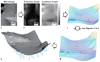 |
Fig. 1 Flow chart of the photoclinometry process. We start with a selected region of a high-resolution NAC image capturing the site of interest (a). Using the NAIF SPICE toolkit, we derive the viewing geometries at this region (b), as well as an initial topology estimate from a shape model (c). We apply a photoclinometry method using the algorithm from Kirk et al. (2003) to derive a detailed topology map (d). Finally, we orthorectify the map and then calculate the local gravity (e). The final image is the topographic surface projected in 3D, with an orthorectified image overlaid on the surface. The arrows are local gravity vectors. The location on the nucleus of the region of interest is shown in Fig. 10. |
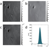 |
Fig. 2 Process of determining the albedo for a region of interest in an image: (a) the original Rosetta NAC image (Imhotep region); (b) simulated image of the same region using the SHAP4S shape model; (c) the “albedo map” created by dividing (a) by (b), and it represents an I/F map of the region; and (d) a histogram of the pixel values in (c). |
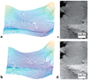 |
Fig. 3 (a) Initial shape model DTM that is used as an estimate, and (b) final DTM after iterative adjustments using the photoclinometry method. The small-scale features are clearly resolved. A comparison of the actual image from the OSIRIS NAC (c) and a simulated image from the final DTM (d). The location on the nucleus of the region of interest is shown in Fig. 10. |
3 Error and validation
To ensure that our DTMs represent the surface of 67P sufficiently well, we undertook two separate tasks. First, we estimated the inherent error within the photoclinometry method so as to ensure that our assumptions did not introduce any artifacts. We then validated the method to ensure repeatability and consistency.
OSIRIS NAC images used in our study.
3.1 Error estimates
Several minor sources of error appear at various stages within the photoclinometry process. The most prominent of these are from inaccuracies of the photometric function because a realistic photometric model is needed to accurately recreate the photometric behavior that produces the shading from slopes. A previous study (Birch et al. 2017), using this method on 67P, compared Hapke models (Hapke 1981, 1984) for the nucleus of 67P (Ciarniello et al. 2015; Fornasier et al. 2015) with the nuclei of 19P/Borrelly (Buratti et al. 2004; Kirk et al. 2004; Li et al. 2007a), 9P/Tempel 1 (Li et al. 2007b), 81P/Wild 2 (Li et al. 2009), and 103P/Hartley (Li et al. 2013) by fitting the empirical Lunar-Lambert function at fixed phase angles (McEwen 1991). They found that employing this photoclinometry method with a Hapke model on 67P can estimate local relief with a vertical precision that is lower than 10% of the pixel size (Birch et al. 2017) for regions that are only confined to the topographically slowly varying smooth terrains.
Anothernecessary assumption that we made was that the photometric properties, especially the albedo, were uniform across the region of interest. Variations in albedo can occur on the surfaces, but their effects can be detected as DTM artifacts consisting of ridges and troughs aligned in the Sun direction (Kirk et al. 2003). Previous studies showed that these artifacts are less severe than comparable ones in dusty regions of Mars (Birch et al. 2017), which are assumed to be photometrically uniform. This provides confidence that our assumption of constant albedo is valid over regions that are several hundred meters wide. The areas used in this study are all within this range.
To estimate the magnitude of these effects, we made ten DTMs of a single, small (smaller than ~ 500 × 500 m) region of smooth terrains within the Imhotep region using the method described in Sect. 2. These images were acquired over many months of the Rosetta mission, with different viewing geometries and illumination conditions (Table 1). All the images were also acquired before April 2015, before any changes occurred (Groussin et al. 2015). Thus, we assume that the surface did not change, which enabled us to check the inherent variability in this method. Finally, these images were acquired over a range of azimuth and phase angles, and at different resolutions, which together resulted in two high-, two intermediate-, and six low-resolution images (Table 1). Because of the vastly different azimuth angle difference for two images in the low-resolution set, which created difficulties in registration, they were accounted for separately. For each set, we then chose one image as our datum and then registered the remainder to match the surface orientation at sub-pixel accuracies. This image registration was done similar to the registration necessary for color image analysis that is described in Appendix A of Oklay et al. (2016).
When our registration was correct, we selected a portion of the DTM 100 m in radius that was fully constrained to smooth terrains, and subtracted the DTMs from each other. The difference between the DTMs is then due to errors generated by the model, and the errors are shown for each of the four sets in Fig. 4. Between images of similar azimuth angles and of the same resolution, the standard deviation of the difference between the DTMs is always lower than the resolution and decreases proportionally for lower-resolution images. The maximum standard deviation is <60 cm for the coarsest images, which is still lower than the typical depth of changes across the nucleus (Sect. 4). This standard deviation is over the pixel scale of the image, which is <1.5 m. For the higher-resolution images, the standard deviation can be as low as 18 cm. This error is easily the largest source of error in this method, but is still sufficiently small for us to produce DTMs that can accurately measure most small-scale changes on the surface of 67P.
Our final error estimate was made to ensure that the model did not produce artificial surfaces. We first generated a high-resolution DTM of a surface region in Hapi (Table 1) using the method described inSect. 2. We then applied a low-pass filter to the DTM, with a box size of 25 × 25 pixels to remove any of the high-resolution topographic features we just iterated on. This produced a new estimate of the surface that very nearly matched the input shape model surface to which the same low-pass filter was applied (Fig. 5). The standard deviation between this DTM and the initial estimate of the surface from the shape model is <0.6 m over large spatial scales (>100 m).
As each of these sources of error are independent of each other, the combined error in our analysis is just each source added in square quadrature. For the coarsest images then, the maximum error in the method is <62 cm, and can be as low as ~18 cm.
These estimates are an upper limit on the error. The inherent variability in this method is likely lower than this. We can estimate the limit of the vertical resolution by measuring the standard deviation of the flattest portion of smooth terrains in Imhotep. To do this, we selected a region 10 × 10 pixels in a high-resolution image (26 cm pixel−1) and then detrended the overall slope. The standard deviation of the elevations within this region is just 10 cm, which is about twice better than our estimate of 18 cm above. Although this may also reflect the true small-scale roughness of the smooth terrains in Imhotep, it provides another estimate, perhaps most realistic, about the standard deviation of the elevation of any given pixel in our DTMs.
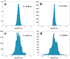 |
Fig. 4 Histograms of the distance between DTMs within the (a) high-resolution set, (b) intermediate-resolution set, and (c and d) low-resolution sets for varying azimuth angles. The standard deviation for each set is given by θ. |
 |
Fig. 5 Left: original shape model DTM with the low-pass filter applied. Right: final DTM with the same low-pass filter applied. The scale across both images is 110 × 160 m. The location on the nucleus of the region of interest is shown in Fig. 10. |
3.2 Validation of DTMs
In order to ensure that this method is consistent and does not introduce any systematic errors, we performed one key check. This test involved using different shape models as the input surface to determine whether there was any dependence on the initial conditions. We used the SHAP2 shape model (Jorda et al. 2016) because it was of lower quality than the shape models produced later in the Rosetta mission. Because there are errors between the shape models themselves, we are no longer concerned with the exact shape of the surface. Instead, the different shape model allows us to clearly determine any errors in the model itself. We thus appliedthis same method and generated two separate DTMs of the same surface (Table 1). Even though they have a different long-wavelength shape because of the difference in the input shape model, the resulting DTMs both reproduce the same high-frequency topography that we are concerned with (Fig. 6).
This shows that at the meter scale, where changes to the smooth terrains occur, the model is insensitive to the initial shape model. Regardless of the initial estimate of the surface, the model can repeatedly generate accurate DTMs. Furthermore, the model does not distort the surface over longer wavelengths.
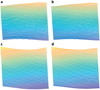 |
Fig. 6 Comparison of the shape model from SHAP4S (top left) and SHAP2 (bottom left), as well as the DTMs derived from them (right). The small-scale features are re-created and the long-wavelength slopes are not distorted. The differences in the long-wavelength slopes between the two final DTMs is from differences between the initial shape models. The scale across all images is 110 × 160 m. The location on the nucleus of the region of interest is shown in Fig. 10. |
4 Application to observed surface changes
Numerous surface changes have been observed on 67P, including jets (Shi et al. 2016; Schmitt et al. 2017), collapse of cliff margins (El-Maarry et al. 2017), scarp retreat (Groussin et al. 2015), emergence and disappearance of ripples (Jia et al. 2017), and movement of large boulders (El-Maarry et al. 2017). Most of these changes, surprisingly, have been within the smooth terrains of 67P, regions that were thought to be relatively inactive. All these changes have a topographic expression that can help inform the process that drives its formation. The larger changes, such as cliff collapses, are captured readily by the existing shape models (Pajola et al. 2017). Many other changes, however, are not because they are at or below even the highest-resolution global meter shape model (Preusker et al. 2017). The photoclinometry method described herein was designed to characterize these types of changes.
Thomas et al. (2015) and Lai et al. (2016) have both examined changes due to gas flow and dust redistribution on the surface of 67P. In addition, Thomas et al. (2015) and Jia et al. (2017) examined features seen within Hapi that appeared like aeolian ripples (Fig. 7a), and theorized that these are formed by diurnal winds from exposure to sunlight. However, ripples are characterized by both a spacing between crests and a consistent topographic form. We generated a DTM of the ripples, as imaged in September 2014, and show that they form crests that range from 0.6−1.3 meters in elevation (Fig. 7b). Because the largest ripples are ~15 meters in width, slopes on the ripples then reach a maximum of ~12°, which is far below the suspected angle of repose (45 ± 5°) (Groussin et al. 2015), but consistent with the model provided by Jia et al. (2017).
Following perihelion, the region was imaged again and showed that the ripple morphology had changed (El-Maarry et al. 2017). Fewer ripples were visible, while they also migrated and changed in orientation with respect to the neighboring cliff (Fig. 7c). This suggests that aeolian processes may not be the dominant formation mechanism because we would expect the ripple spacing and number of ripples to remain consistent. We made a DTM of these new ripples and found that they range in elevation from 14−60 cm (Fig. 7d), which is substantially lower than the previous image. Together, these results suggest that the process responsible for the formation of the ripples does not consistently create the same feature, despite their curious reappearance at the same location. This may point to other processes, such as removal of inter-ripple material into underlying fractures emanating from the nearby cliff. In this manner, the ripples would just be material left behind, and the features would be more analogous to lineations on Phobos and other small bodies (Buczkowski 2006). These features should be explored in further detail considering the new observations.
Other changes were also cataloged by Hu et al. (2017) within smooth terrains, termed “honeycomb” because their morphologic appearance is similar. Hu et al. (2017) then correlated their appearances with other known factors such as illumination and temperature conditions, but left a formation model an open question. An accurate representation of their surfaces, which we provide in Fig. 8, before and after the changes, should assist in developing models of these peculiar features. We note, however, from Fig. 8 that the features are not a representation of the underlying rough bedrock, as the feature is of positive relief. If the honeycomb feature were depressed compared to the surrounding, then the interpretation that it was exposed, underlying bedrock may be correct. Instead, an unknown mechanism has roughened the same surface of smooth terrain.
The sudden appearance and disappearance of depressions with the smooth terrains also occurred throughout the Rosetta mission (Groussin et al. 2015; El-Maarry et al. 2017) (Birch et al., in prep.), and they are perhaps the most dramatic type of changes to occur within smooth terrains. Unfortunately, the origin and migration of these features remain difficult for models to explain because topographic information is scarcely available. We therefore made a DTM of the depressions in Imhotep and Hapi and show that they have depths of ~1.1 m (Fig. 9). Similar changes were also observed in the Hapi region some months before perihelion, which show depths of 0.4−1.5 m (Birch et al. 2019), comparable to the depth of the others that we measured (Fig. 9). These depths are all deeper than the thermal skin depth (Shi et al. 2016), suggesting an additional dynamical process that is able to excavate to such substantial depths. This will be further discussed in a follow-up paper that investigates the origin and evolution of these features in detail (Birch et al., in prep.).
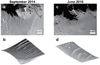 |
Fig. 7 Panel a: OSIRIS NAC image of ripples within the Hapi region as imaged in September 2014. Panel b: DTM of the ripples. The top right side is removed before the DTM was generated because the cliffs of the Seth region intruded on the region of the ripples. Panel c: OSIRIS NAC image of ripples as imaged in June 2016. Fewer ripples are in the region, and they have changed location and orientation relative to the cliff. Panel d: DTM of the ripples. The location on the nucleus of the region of interest is shown in Fig. 10. |
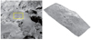 |
Fig. 8 Left: OSIRIS NAC image of the honeycomb features on 28 March 2015. Right: the DTM we generate shows that these features are positive in relief, suggesting an erosive mechanism that can incise through the smooth terrains. The scale across the DTM is 257 × 103 m. The location on the nucleus of the region of interest is shown in Fig. 10. |
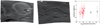 |
Fig. 9 Left: DTM of the depression within Imhotep. The scale across the DTM is 361 × .433 m. Middle: DTM of the depression within Hapi. The scale across the DTM is 110 × 160 m. Right: depression depths as a function of their area. All depressions appear to range from 50 cm to 1.5 m in depth. Points in red are measured from Birch et al. (in prep.), and those in black are measured from the depressions in the left and middle panels. The thin error bars are as measured in Sect. 3.1, and the thick error bars represent the more realistic error inherent in our method (~10 cm). The locations on the nucleus of the regions of interest are shown in Fig. 10. |
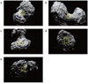 |
Fig. 10 Locations of Rosetta NAC images used in this paper. (a) Figures 1 and 3; (b) Fig. 7; (c) Fig. 8; (d) Fig. 9 (left); and (e) Figs. 5, 6, and 9 (middle). |
5 Conclusions
We presented a method for generating high-resolution DTMs, both vertically and spatially, of smooth terrain regions on 67P. As these appear to be the most active regions of the nucleus (El-Maarry et al. 2017; Vincent & Team 2018), the ability to generate sufficient topography is critical to understanding their origin and evolution. This model allowed us to reliably produce DTMs of these surfaces, and it provides estimates to the error as well, which should enable detailed and quantifiable measurements of any type of surface change within smooth terrains.
In using the described algorithm to examine the ripples, honeycomb, and depressions, we also demonstrated its utility to investigate small-scale changes on 67P. These DTMs show that the depth that changes excavate to is often smaller than one meter, suggesting additional as yet unknown dynamical mechanisms that can excavate to such depths. Furthermore, the capabilities of the model are not limited to the features we examined in this study, and can be used extensively in a variety of situations, including other surface features and changes on 67P, and other bodies that are photometrically uniform over small spatial scales where changes may occur (e.g., 162173 Ryugu and 101955 Bennu).
Acknowledgements
This research was supported by Cornell University and NASA’s CAESAR science team. We would also like to acknowledge the Principal Investigator of the OSIRIS camera on ESA’s Rosetta spacecraft, Holger Sierks, and the ESA Planetary Science Archive for the data used in this study. This research has made use of the scientific software shapeViewer (www.comet-toolbox.com).
References
- Acton, C. H. 1996, Planet. Space Sci., 44, 65 [NASA ADS] [CrossRef] [Google Scholar]
- Birch, S. P. D., Tang, Y., Hayes, A. G., et al. 2017, MNRAS, 469, S50 [CrossRef] [Google Scholar]
- Birch, S., Hayes, A., Umurhan, O., et al., 2019, Lunar Planet. Sci. Conf., 50, 2106 [NASA ADS] [Google Scholar]
- Buczkowski, D. L. 2006, Johns Hopkins APL Technical Digest, 27, 100 [Google Scholar]
- Buratti, B., Hicks, M., Soderblom, L., et al. 2004, Icarus, 167, 16 [NASA ADS] [CrossRef] [Google Scholar]
- Ciarniello, M., Capaccioni, F., Filacchione, G., et al. 2015, A&A, 583, A31 [NASA ADS] [CrossRef] [EDP Sciences] [Google Scholar]
- El-Maarry, M. R., Groussin, O., Thomas, N., et al. 2017, Science, 355, 1392 [NASA ADS] [CrossRef] [Google Scholar]
- Fornasier, S., Hasselmann, P. H., Barucci, M. A., et al. 2015, A&A, 583, A30 [NASA ADS] [CrossRef] [EDP Sciences] [Google Scholar]
- Groussin, O., Sierks, H., Barbieri, C., et al. 2015, A&A, 583, A36 [NASA ADS] [CrossRef] [EDP Sciences] [Google Scholar]
- Hapke, B. 1981, J. Geophys. Res. Solid Earth, 86, 3039 [NASA ADS] [CrossRef] [Google Scholar]
- Hapke, B. 1984, Icarus, 59, 41 [NASA ADS] [CrossRef] [Google Scholar]
- Hu, X., Shi, X., Sierks, H., et al. 2017, A&A, 604, A114 [NASA ADS] [CrossRef] [EDP Sciences] [Google Scholar]
- Jia, P., Andreotti, B., & Claudin, P. 2017, Proc. Natl. Acad. Sci., 114, 2509 [NASA ADS] [CrossRef] [Google Scholar]
- Jorda, L., Gaskell, R., Capanna, C., et al. 2016, Icarus, 277, 257 [NASA ADS] [CrossRef] [Google Scholar]
- Keller, H. U., Arpigny, C., Barbieri, C., et al. 1986, Nature, 321, 320 [NASA ADS] [CrossRef] [Google Scholar]
- Keller, H. U., Barbieri, C., Lamy, P., et al. 2007, Space Sci. Rev., 128, 433 [NASA ADS] [CrossRef] [Google Scholar]
- Kirk, R. L., Howington-Kraus, E., Redding, B., et al. 2003, J. Geophys. Res.: Planets, 108 [Google Scholar]
- Kirk, R. L., Howington-Kraus, E., Soderblom, L. A., Giese, B., & Oberst, J. 2004, Icarus, 167, 54 [NASA ADS] [CrossRef] [Google Scholar]
- Lai, I.-L., Ip, W.-H., Su, C.-C., et al. 2016, MNRAS, 462, S533 [CrossRef] [Google Scholar]
- Li, J.-Y., A’Hearn, M. F., McFadden, L. A., & Belton, M. J. 2007a, Icarus, 188, 195 [NASA ADS] [CrossRef] [Google Scholar]
- Li, J.-Y., A’Hearn, M. F., Belton, M. J., et al. 2007b, Icarus, 187, 41 [NASA ADS] [CrossRef] [Google Scholar]
- Li, J.-Y., A’Hearn, M. F., Farnham, T. L., & McFadden, L. A. 2009, Icarus, 204, 209 [NASA ADS] [CrossRef] [Google Scholar]
- Li, J.-Y., Besse, S., A’Hearn, M. F., et al. 2013, Icarus, 222, 559 [NASA ADS] [CrossRef] [Google Scholar]
- McEwen, A. S. 1991, Icarus, 92, 298 [NASA ADS] [CrossRef] [Google Scholar]
- Oklay, N., Vincent, J.-B., Fornasier, S., et al. 2016, A&A, 586, A80 [NASA ADS] [CrossRef] [EDP Sciences] [Google Scholar]
- Pajola, M., Höfner, S., Vincent, J. B., et al. 2017, Nat. Astron., 1, 0092 [CrossRef] [Google Scholar]
- Preusker, F., Scholten, F., Matz, K.-D., et al. 2015, A&A, 583, A33 [NASA ADS] [CrossRef] [EDP Sciences] [Google Scholar]
- Preusker, F., Scholten, F., Matz, K.-D., et al. 2017, A&A, 607, L1 [NASA ADS] [CrossRef] [EDP Sciences] [Google Scholar]
- Schmitt, M. I., Tubiana, C., Güttler, C., et al. 2017, MNRAS, 469, S380 [CrossRef] [Google Scholar]
- Shi, X., Hu, X., Sierks, H., et al. 2016, A&A, 586, A7 [NASA ADS] [CrossRef] [EDP Sciences] [Google Scholar]
- Shi, X., Hu, X., Mottola, S., et al. 2018, Nat. Astron., 2, 562 [NASA ADS] [CrossRef] [Google Scholar]
- Sierks, H., Barbieri, C., Lamy, P. L., et al. 2015, Science, 347 [Google Scholar]
- Thomas, P., A’Hearn, M., Belton, M., et al. 2013, Icarus, 222, 453 [NASA ADS] [CrossRef] [Google Scholar]
- Thomas, N., Davidsson, B., El-Maarry, M. R., et al. 2015, A&A, 583, A17 [NASA ADS] [CrossRef] [EDP Sciences] [Google Scholar]
- Veverka, J., Klaasen, K., A’Hearn, M., et al. 2013, Icarus, 222, 424 [NASA ADS] [CrossRef] [Google Scholar]
- Vincent, J.-B. & Team, O. 2018, in 49th Lunar and Planetary Science Conference (Houston: Lunar and Planetary Institute), Abstract #1280 [Google Scholar]
- Vincent, J.-B., Bodewits, D., Besse, S., et al. 2015, Nature, 523, 63 [NASA ADS] [CrossRef] [Google Scholar]
- Werner, R. A., & Scheeres, D. J. 1997, Celest. Mech. Dyn. Astron., 65, 313 [NASA ADS] [CrossRef] [Google Scholar]
All Tables
All Figures
|
Fig. 1 Flow chart of the photoclinometry process. We start with a selected region of a high-resolution NAC image capturing the site of interest (a). Using the NAIF SPICE toolkit, we derive the viewing geometries at this region (b), as well as an initial topology estimate from a shape model (c). We apply a photoclinometry method using the algorithm from Kirk et al. (2003) to derive a detailed topology map (d). Finally, we orthorectify the map and then calculate the local gravity (e). The final image is the topographic surface projected in 3D, with an orthorectified image overlaid on the surface. The arrows are local gravity vectors. The location on the nucleus of the region of interest is shown in Fig. 10. |
| In the text | |
|
Fig. 2 Process of determining the albedo for a region of interest in an image: (a) the original Rosetta NAC image (Imhotep region); (b) simulated image of the same region using the SHAP4S shape model; (c) the “albedo map” created by dividing (a) by (b), and it represents an I/F map of the region; and (d) a histogram of the pixel values in (c). |
| In the text | |
|
Fig. 3 (a) Initial shape model DTM that is used as an estimate, and (b) final DTM after iterative adjustments using the photoclinometry method. The small-scale features are clearly resolved. A comparison of the actual image from the OSIRIS NAC (c) and a simulated image from the final DTM (d). The location on the nucleus of the region of interest is shown in Fig. 10. |
| In the text | |
|
Fig. 4 Histograms of the distance between DTMs within the (a) high-resolution set, (b) intermediate-resolution set, and (c and d) low-resolution sets for varying azimuth angles. The standard deviation for each set is given by θ. |
| In the text | |
|
Fig. 5 Left: original shape model DTM with the low-pass filter applied. Right: final DTM with the same low-pass filter applied. The scale across both images is 110 × 160 m. The location on the nucleus of the region of interest is shown in Fig. 10. |
| In the text | |
|
Fig. 6 Comparison of the shape model from SHAP4S (top left) and SHAP2 (bottom left), as well as the DTMs derived from them (right). The small-scale features are re-created and the long-wavelength slopes are not distorted. The differences in the long-wavelength slopes between the two final DTMs is from differences between the initial shape models. The scale across all images is 110 × 160 m. The location on the nucleus of the region of interest is shown in Fig. 10. |
| In the text | |
|
Fig. 7 Panel a: OSIRIS NAC image of ripples within the Hapi region as imaged in September 2014. Panel b: DTM of the ripples. The top right side is removed before the DTM was generated because the cliffs of the Seth region intruded on the region of the ripples. Panel c: OSIRIS NAC image of ripples as imaged in June 2016. Fewer ripples are in the region, and they have changed location and orientation relative to the cliff. Panel d: DTM of the ripples. The location on the nucleus of the region of interest is shown in Fig. 10. |
| In the text | |
|
Fig. 8 Left: OSIRIS NAC image of the honeycomb features on 28 March 2015. Right: the DTM we generate shows that these features are positive in relief, suggesting an erosive mechanism that can incise through the smooth terrains. The scale across the DTM is 257 × 103 m. The location on the nucleus of the region of interest is shown in Fig. 10. |
| In the text | |
|
Fig. 9 Left: DTM of the depression within Imhotep. The scale across the DTM is 361 × .433 m. Middle: DTM of the depression within Hapi. The scale across the DTM is 110 × 160 m. Right: depression depths as a function of their area. All depressions appear to range from 50 cm to 1.5 m in depth. Points in red are measured from Birch et al. (in prep.), and those in black are measured from the depressions in the left and middle panels. The thin error bars are as measured in Sect. 3.1, and the thick error bars represent the more realistic error inherent in our method (~10 cm). The locations on the nucleus of the regions of interest are shown in Fig. 10. |
| In the text | |
Current usage metrics show cumulative count of Article Views (full-text article views including HTML views, PDF and ePub downloads, according to the available data) and Abstracts Views on Vision4Press platform.
Data correspond to usage on the plateform after 2015. The current usage metrics is available 48-96 hours after online publication and is updated daily on week days.
Initial download of the metrics may take a while.