| Issue |
A&A
Volume 630, October 2019
|
|
|---|---|---|
| Article Number | A84 | |
| Number of page(s) | 17 | |
| Section | Interstellar and circumstellar matter | |
| DOI | https://doi.org/10.1051/0004-6361/201833400 | |
| Published online | 24 September 2019 | |
New insight on accretion shocks onto young stellar objects
Chromospheric feedback and radiation transfer
1
LERMA, Sorbonne Universités, Observatoire de Paris, PSL Research University, CNRS,
75252
Paris,
France
e-mail: This email address is being protected from spambots. You need JavaScript enabled to view it.
2
CEA/IRFU/SAp, CEA Saclay, Orme des Merisiers,
91191
Gif-sur-Yvette,
France
3
Steward Observatory, University of Arizona, 933 North Cherry Avenue,
Tucson,
AZ
85721,
USA
4
Observatoire de la Côte d’Azur (OCA),
06304
Nice,
France
5
LUTh, Observatoire de Paris, PSL University, CNRS, Paris-Diderot University,
Meudon,
France
Received:
9
May
2018
Accepted:
15
August
2019
Abstract
Context. Material accreted onto classical T Tauri stars is expected to form a hot quasi-periodic plasma structure that radiates in X-rays. Simulations of this phenomenon only partly match observations. They all rely on a static model for the chromosphere and on the assumption that radiation and matter are decoupled.
Aims. We explore the effects of a shock-heated chromosphere and of the coupling between radiation and hydrodynamics on the structure and dynamics of the accretion flow.
Methods. We simulated accretion columns that fall onto a stellar chromosphere using the 1D ALE code AstroLabE. This code solves the hydrodynamics equations along with the first two moment equations for radiation transfer, with the help of a dedicated opacity table for the coupling between matter and radiation. We derive the total electron and ion densities from collisional-radiative model.
Results. The chromospheric acoustic heating affects the duration of the cycle and the structure of the heated slab. In addition, the coupling between radiation and hydrodynamics leads to a heating of the accretion flow and of the chromosphere: the whole column is pushed up by the inflating chromosphere over several times the steady chromosphere thickness. These last two conclusions are in agreement with the computed monochromatic intensity. Acoustic heating and radiation coupling affect the amplitude and temporal variations of the net X-ray luminosity, which varies between 30 and 94% of the incoming mechanical energy flux, depending on which model is considered.
Key words: stars: pre-main sequence / accretion, accretion disks / methods: numerical / hydrodynamics / radiative transfer / opacity
Deceased.
© L. de Sá et al. 2019
 Open Access article, published by EDP Sciences, under the terms of the Creative Commons Attribution License (http://creativecommons.org/licenses/by/4.0), which permits unrestricted use, distribution, and reproduction in any medium, provided the original work is properly cited.
1 Introduction
Classical T Tauri stars (CTTSs) are solar-type pre-main-sequence stars that are surrounded by a thick disc composed of gas and dust (see e.g. Feigelson & Montmerle 1999). Disc material follows a near-Keplerian infall down to the truncation radius, at which thermal and magnetic pressures balance. Free-falling material then flows from the inner disc down to the stellar surface in magnetically confined accretion columns (Calvet & Gullbring 1998). Hot-spot observations (Gullbring et al. 2000) suggest filling factors of up to 1% (Bouvier et al. 1995).
Accreted gas is stopped at the balance of the ram pressure of the flow and of the thermal pressure of the stellar chromosphere: a forward shock forms, and the post-shock material accumulates at the basis of the column. The hot slab of post-shock material is separated from the accretion flow by a reverse shock (which is sometimes ambiguously called accretion shock). A typical simulated structure of an accretion shock can be found for instance in Orlando et al. (2010) and is sketched in Fig. 1.
One of the most direct probes for the accretion process comes from the X-rays that are emitted by the dense (ne > 1011 cm−3) and hot (Te ≃ 2−5 MK) post-shock plasma (see Kastner et al. 2002 and Stelzer & Schmitt 2004 for TW Hya, Schmitt et al. 2005 for BP Tau, Günther et al. 2006 for V4046 Sgr, Argiroffi et al. 2007, 2009 for MP Mus, Robrade & Schmitt 2007 for RU Lup, and Huenemoerder et al. 2007 for Hen 3-600). Another signature is the UV and optical veiling, which is attributed to the post-shock medium, the heated atmosphere, and the pre-shock medium (Calvet & Gullbring 1998). In addition, Doppler profiles of several emission lines trace the high velocity in the funnelled flow (up to 500 km s−1, according to Muzerolle et al. 1998).
One-dimensional hydrodynamical models (Sacco et al. 2008, 2010) predict quasi-periodic oscillations (QPOs) of the post-shock slab with periods ranging from 0.01 to 1000 s, depending on the inflow density, metallicity, velocity, and inclination with respect to the stellar surface. For a typical free-fall radial velocity of 400 km s−1, Sacco et al. (2010) for instance found a period of 160 s at 1011 cm−3. These oscillations are triggered by the cooling instability (for further details, see e.g. Chevalier & Imamura 1982; Walder & Folini 1996; Mignone 2005).
Although plasma characteristics derived from X-ray observations are consistent with the density and the temperature predicted by these numerical studies, there is no obvious observational evidence for this periodicity. Drake et al. (2009) thoroughly studied soft X-ray emission from TW Hya and found no periodicity in the range 0.0001–6.811 Hz. Günther et al. (2010) completed this study with optical and UV emission, and they came to the same conclusion in the range 0.02–50 Hz. However, a recent photometric study of TW Hya based on observations obtained with the Microvariability and Oscillations of Stars telescope (MOST) reports possible oscillations with a period of 650–1200 s, which might be attributed to post-shock plasma oscillations (Siwak et al. 2018).
Observations thus raise the question of the existence of an oscillating hot slab in the accretion context. Several numerical studies explored multi-dimensional magnetic effects, such as leaks at the basis of the column (Orlando et al. 2010), the taperingof the magnetic field (Orlando et al. 2013), or perturbations in the flow (Matsakos et al. 2013). Although QPOs are still obtained in these numerical studies, the accretion funnel basis is either fragmented in out-of-phasefibrils, or sunk below a cooler and denser gas layer that strongly absorbs X-rays. The observation of global synchronous QPOs therefore becomes very challenging (Curran et al. 2011; Bonito et al. 2014; Colombo et al. 2016; Costa et al. 2017). Consequences of the slab sinking in the chromosphere have also been explored in several 1D simulations (Drake 2005; Sacco et al. 2010). When the slab is deeply sunk, the radiation may only escape the post-shock structure from its upper part. The X-ray luminosity may therefore be significantly reduced.
In thesenumerical works, the accretion is assumed to take place onto a quiet medium (an isothermal atmosphere in the best cases). Moreover, the post-shock medium is assumed to be optically thin, and the coupling between radiation and matter is then reduced to a cooling function for the gas (see e.g. Kirienko 1993). Although this assumption can be justified to model the infalling gas and the post-shock plasma, it is inconsistent with any stellar atmosphere model. The energy balance between radiation and gas in the lower stellar atmosphere is then replaced by a non-physical tuning (heating function, off threshold, etc.). Such an assumption may affect the sinking of the post-shock structure as well as the accretion structure itself.
We here focus and refine the physics that is encompassed in existing 1D models. We first explore the effect of perturbations by chromospheric shocks on the accretion dynamics. We then analyse how radiation may affect the chromospheric, post-shock, and accreted plasmas as well as the QPO duration and the depth of the hot slab in the chromosphere; we also synthesise and discuss the accretion signature in the emerging radiative spectra. In Sect. 2 we present the radiation hydrodynamics model and the numerical tools we used. We detail in Sect. 2.2.3 the two extreme radiative regimes we encountered in this context and describe a simple model for intermediate radiative regimes. Section 3 is dedicated to accretion simulations and to the corresponding discussions. The last section (Sect. 4) presents caveats and possible improvements to this work.
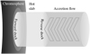 |
Fig. 1 Sketch of the basis of an accretion column and its three distinctive zones: the chromosphere (left, dark grey), the accretion flow (right, mid-grey) and the zone in between (middle, light grey), hereafter called hot slab or post-shock medium. |
2 Physical and numerical models
Our model is based on the conservation equations of hydrodynamics (Sect. 2.1.1). These equations include the contributions of the radiation energy and flux that are derived from the moment equations (Sect. 2.2.2). Ionisation is included in the equation of state and in the gas energy balance (Sect. 2.1.2).
2.1 Hydrodynamics model
2.1.1 Hydrodynamics equations
We consider a star of radius R⋆ and mass M⋆. The accreted and stellar atmospheric plasmas at position r ( ), hereafter taken from the stellar surface, are characterised by a (volumetric mass) density ρ, a velocity v, a thermal pressure p, and a volumetric internal energy density e. The plasma evolution is modelled by solving the hydrodynamics equations, written in the conservative form:
![Mathematical equation: \begin{equation*}\left\{\begin{array}{@{}r@{\,}l@{}r@{\,}l@{\,}l} \partial_t\rho &+\vec{\nabla}\cdot&(\rho\,\vec{v}) &= 0,\\[3pt] \partial_t(\rho\,\vec{v}) &+\vec{\nabla}&\hspace{-3pt}(\rho\,\vec{v}\otimes\vec{v}) &= \vec{\mathfrak{s}}_{\mathrm{m}} &= -\vec{\nabla}\left(p+p_{\mathrm{vis}}\right) + \vec{g}(\vec{r}) - \vec{\mathfrak{s}}_{M_{\mathrm{r}}},\\[3pt] \partial_t e &+\vec{\nabla}\cdot& (e\,\vec{v}) &= \mathfrak{s}_{\mathrm{e}} & = - \vec{\nabla}\cdot\left(p\,\vec{v}\right) + q_{\mathrm{vis}} - \vec{\nabla}\cdot \vec{q}_{\mathrm{\!C}} - \mathfrak{s}_{E_{\mathrm{r}}} - q_{\chi}, \end{array}\right.\hspace{-3em} \end{equation*}](/articles/aa/full_html/2019/10/aa33400-18/aa33400-18-eq2.png) (1)
(1)
with  .
.
The gas source terms (𝔰e and 𝔰m, which can be either positive or negative) include the contributions of thermal conduction (qC, Spitzer & Härm 1953; Vidal et al. 1995), gravity (g(r)), artificial viscosity (pvis and qvis, von Neumann & Richtmyer 1950), and the coupling with radiation ( and
and  , see Sect. 2.2.3). The closure relation for this system of equations (the equation of state) is adapted from the ideal gas law: p = ntot k T ⇔ e = 3∕2 p, where ntot stands for the total volumetric number density of free particles (neutrals, electrons, and ions), and T represents their kinetic temperature (all particles are assumed here to have the same kinetic temperature: Tneutrals = Tions = Telectrons = T). The contributionof ionisation and recombination on the gas energy density is included in the thermochemistry term qχ and is discussed in Sect. 2.1.2.
2.1.2 Collisional-radiative ionisation
The forward shock forms where the ram pressure is balanced by the local thermal pressure, thus within the stellar chromosphere that then needs to be modelled. In contrast to the solar case, information about T Tauri chromospheres is very limited. Because our goal is to propose a qualitative description of the dynamics of this chromosphere and in absence of any reliable information, our chromospheric model (see Appendix B) is therefore inspired by the solar case. We also chose for simplicity solar abundances taken from Grevesse & Sauval (1998), even though the chemical abundance of the accreted matter is expected to be more complex (Fitzpatrick 1996; Günther et al. 2007; Güdel et al. 2007; Güdel 2008). In the hydrodynamics, we only considered hydrogen (H I, H II) and helium (He I, He II, He III); the chemical composition is completed by a “catch-all” metal “M” with a number abundance of 0.12% and a mass (averaged over abundances) of 17 u.
Most simulations are performed using time-independent ionisation models, for instance the modified Saha equilibrium of Brown (1973) (see e.g. Sacco et al. 2008) or a detailed collisional ionisation calculation (e.g. Günther et al. 2007). To estimate the total free electron density ne in the two first setups, we used the modified Saha model (for which qχ = 0).
The last simulation presented in this paper (referred to as the Hybrid setup) uses a time-dependent collisional-radiative ionisation model with collisional ionisation rates given by Voronov (1997), radiative recombination rates computed by Verner & Ferland (1996), helium dielectronic recombination rate proposed by Hui & Gnedin (1997), and photoionisation rates (P) derived from Spitzer (1998) and Yan et al. (1998) cross-sections, along with the local radiation energy density. The time-dependent ion and neutral volumetric number densities n were computed by a conservative set of equations (see e.g. Eq. (1)). The electron volumetric number density was derived from the neutrality conservation: ne = nHe II + nHe II + 2 nHe III. Finally, the thermochemistry term qχ sums all these contributions, weighted by the corresponding gained or lost energy.
2.2 Radiation model
2.2.1 Radiation and hydrodynamics
The coupling between radiation and matter enters at different scales in astrophysical plasmas. At a microscopic scale, radiation affects the thermodynamical state of the matter through its contribution to the populations of the electronic energy levels of each plasma ion. The computation of these populations is based on a large set of kinetic equilibrium equations that take into account excitation and de-excitation processes due to collisions (interactions with massive particles, mostly electrons) as well as radiative processes (interactions with photons). This step allowed us to derive the monochromatic absorption and emission coefficients as well, κν (also called monochromatic opacity, in cm2 g−1) and ην (in erg cm−3 s−1), respectively,which in turn were used to compute the local radiation intensity by solving the equations of radiative transfer. Two limiting (and simplifying) cases are expected: at high electron densities, local thermodynamic equilibrium (LTE) is recovered, whereas at low density and for an optically thin medium, the coronal limit is reached (Oxenius 1986).
The main issue in performing such calculations is an intricate coupling between the kinetic equilibrium equations (easily solved given the radiation field) and the radiative transfer equation (simple to calculate when the atomic level populations and hence the absorption and emission coefficients are known). Because a mean free path of photons is typically much larger than the mean free path of massive particles, an explicit treatment of the radiation transport necessarily involves a significant non-locality of the problem. This problem is satisfactorily solved in the case of stationary stellar atmospheres (see e.g. Hubeny & Mihalas 2014) through efficient iterative methods. However, this remains difficult in the case of a non-stationary plasma, where the equations of hydrodynamics each time need to be coupled with the equations for the radiative transfer.
The previous kinetic equations therefore have to be solved simultaneously with the monochromatic radiative transfer equations. This allows computing the frequency-averaged local radiation energy, flux, and pressure, and helps to include these quantities in the hydrodynamics equations (Eq. (1)). In practice, this exact description would require extensive numerical resources: the difficulty is commonly reduced by averaging the radiation quantities by frequency bands. In the multi-group approximation, the absorption and emission coefficients are averaged over several frequency bands using adapted weighting functions: the larger the number of groups, the better the precision of the computation. The simplest and most commonly used approach is the monogroup approximation, which means that the radiation quantities are averaged over the whole frequency domain.
In addition to these delicate issues, radiative transfer takes part in the computation of the spectrum that emerges from this structure. This is commonly done by post-processing the hydrodynamic results by more detailed spectral synthesis tools, as detailed in Sect. 2.3.3.
2.2.2 Moment equations
The radiation field is described here by the momenta equations (see e.g. Mihalas & Mihalas 1984) for the frequency-integrated radiation energy volumetric density (Er, in erg cm−3) and momentum (Mr, in erg cm−4 s) or flux (Fr = c2Mr, in erg cm−2 s−1), written in the comoving frame (Lowrie et al. 2001):
![Mathematical equation: \begin{equation*}\newcommand{\scdot}{\!\cdot\!} \left\{\!\!\!\begin{array}{l} \partial_t E_{\mathrm{r}} +\vec{v}\scdot\partial_t\vec{M}_{\mathrm{\!r}} +c^2\vec{\nabla}\scdot\vec{M}_{\mathrm{\!r}} +\left(\tens{P}_{\mathrm{\!r}}\!:\vec{\nabla}\right)\scdot\vec{v} + \vec{\nabla}\scdot\left(E_{\mathrm{r}}\,\vec{v}\right) = \mathfrak{s}_{E_{\mathrm{r}}},\\[5pt] \partial_t \vec{M}_{\mathrm{\!r}} +\vec{v}\scdot\partial_t\tens{P}_{\mathrm{\!r}}/c^2 +\vec{\nabla}\scdot\tens{P}_{\mathrm{\!r}} +\left(\vec{M}_{\mathrm{\!r}}\cdot\vec{\nabla}\right) \vec{v} + \vec{\nabla} \left(\vec{M}_{\mathrm{\!r}}\scdot\vec{v}\right) = \vec{\mathfrak{s}}_{M_{\mathrm{r}}}. \end{array}\right.\hspace{-1em} \end{equation*}](/articles/aa/full_html/2019/10/aa33400-18/aa33400-18-eq6.png) (2)
(2)
The (monogroup) radiation quantities are integrated from 1 Å to 104 Å. The M1 closure relation then allows us to derive the radiation pressure Pr from the radiation energy density: Pr = D Er. D and χ are the Eddington tensor and factor (D ≡ χ in 1D), respectively, and are defined as follows:
 (3)
(3)
with the reduced flux f =Fr∕(c Er) (and f = || f||), the flux direction i =f∕f =Fr∕Fr, and I2 the second-order identity tensor. As a drawback, the M1 radiation transfer may not properly model the radiation field in structures that involve more than one main radiation source (see e.g. Jiang et al. 2014a,b; Sądowski et al. 2014). Moreover, in contrast to the radiation energy, the contribution of the radiation flux to the hydrodynamics is not straightforward to interpret (for instance, in the case of an isotropic radiation, Fr =0 whereas the radiation energy can be high). Both are presented and discussed with our last setup (Radiation energy and flux section).
Depending on the expression of the radiation source terms, these equations can continuously model optically thin to thick propagation media (see e.g. Mihalas & Mihalas 1984).
2.2.3 Radiation source terms: opacities and line cooling
We aim to describe a system that is composed of three zones in a consistent way. These zones are coupled together through radiation but are in different thermodynamical states (Fig. 1): the dense and optically thick near-LTE chromosphere (Optically thick limit section) on the one hand, and the optically thin coronal hot accretion slab and cold accretion flow (Optically thin limit section) on the other hand. We also expect, according to Calvet & Gullbring (1998), for instance, that the frequency distribution of the measured radiation varies strongly from the X-rays to the infrared. We decided to proceed step by step, using a model that makes a continuous transition between the optically thick LTE approximation and the coronal limit, as described in Intermediate regimes section.
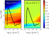 |
Fig. 2 Planck (κP, left) and Rosseland (κR, right) opacities with respect to gas density and temperature, in log scale (see Appendix A). The black curve represents typical conditions in the chromosphere, accretion shock, and flow. |
Optically thick limit
The deep stellar atmosphere is optically thick and can be considered at LTE: each microphysics process is counter-balanced by its reverse process. In LTE and regimes close to LTE, the monochromatic absorption and emission coefficients are linked through the Planck distribution function ην = κν ρ c Bν. The radiation energy and momentum source terms are then defined by (see e.g. Mihalas & Mihalas 1984)
 (4)
(4)
where aR is the radiation constant. Two radiation-matter coupling factors appear here (in cm2 g−1). The Planck mean opacity κP is based on the frequency-integrated absorption coefficient κν weighted by the Planck distribution function Bν, while the Rosseland mean opacity κR is the harmonic mean of κν weighted by the temperature derivative of the Planck function ∂TBν, as follows (Mihalas & Mihalas 1984):
 (5)
(5)
In these frequency averages, the Planck mean is dominated by strong absorption features (typically lines), whereas the Rosseland mean is dominated by the regions in the spectrum of lowest monochromatic opacity. As a consequence, at large optical depths, κP correctly describes the energy exchange between particles and photons, while κR gives the correct total radiative flux (Hubeny & Mihalas 2014).
Several opacity tables are available for a variety of chemical compositions. However, they all fail to cover the full (ρ, T) domain explored in our simulations (see solid black line in Fig. 2). We therefore constructed our own LTE opacity table (see Appendix A for further details) that we present in Fig. 2 with the SYNSPEC code (Sect. 2.3.3). These opacities include atomic (high T) and molecular (low T) contributions.
Optically thin limit
Because of its very low density (ρ ≃ 10−13 g cm−3), the accretedplasma can be described by the limit regime where the gas density tends towards zero: the coronal regime. The coupling between radiation and matter is in this case reduced to an optically thin radiative cooling function Λ(T) (in erg cm3 s−1). In Eq. (2), the radiation source terms become
 (6)
(6)
The first quantity represents the net radiation power emitted by unit volume in all directions (4πsr) by a hot optically thin plasma (in erg cm−3 s−1 sr−1). The term  is set to zero because radiation and matter are not coupled in this regime (see Appendix C for more details).
Our work is based on the cooling function provided by Kirienko (1993), reproduced in Fig. 3, with Z∕Z⊙ = 1 (see Appendix B.1 for the explanation).
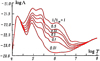 |
Fig. 3 Optically thin radiative cooling (in erg cm3 s−1) for different metallicities Z versus gas temperature (K), adapted from Kirienko (1993). |
Intermediate regimes
The previous source terms describe two well-defined plasma situations. On the one hand, the basis of the stellar chromosphere is optically thick and can be described by the previous LTE radiation source terms. On the other hand, the low-density hot slab is mostly optically thin and can be described in the coronal regime.
It is physically expected and numerically compulsory to perform a smooth and continuous transition to encompass intermediate regimes. This could be done using adequate opacities and emissivities, such as are obtained in a collisional-radiative model. This is unfortunately not yet available for the whole range of physical conditions of our study.
We therefore preferred to follow the transition between LTE and coronal regimes with the probability for a photon (emitted from the column centre) to escape sideways (see e.g. Lequeux 2005, Eq. (3.66)):
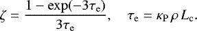 (7)
(7)
ρ and κP values are taken at the photon emission position. The characteristic length Lc is here taken as the accretion column mean radius (typically 1000 km, see Sect. 3.1). Radiation source terms then become (see Appendix C for further details)
 (8)
(8)
the asterisk and dagger denote the LTE (Eq. (4)) and the coronal (Eq. (6)) expressions, respectively.
2.3 Numerical tools
2.3.1 One-dimensional approach
Observations indicate that, in general, the ambient magnetic field is of the order of 1 kG (Johns-Krull et al. 1999; Johns-Krull 2007). The resulting Larmor radius (1 mm) is very small, and the plasma then follows the magnetic field lines. Moreover, the Alfvén velocity reaches 3% of the speed of light and the magnetic waves therefore behave like usual light waves. When we focus on the heart of an accretion column in strong magnetic field case, we can accordingly model the accreted material along one field line, which we assumed to be radial relative to the stellar centre. In our simulations, we therefore only consider the radial component of vector quantities. Because the accretion process is expected to involve strong shocks, we chose a numerical tool that can achieve very high spatial resolution.
Characteristics of the three simulations and their main results.
2.3.2 AstroLabE: an ALE code
Our work is based on numerical studies performed with the 1D arbitrary-Lagrangian-Eulerian (ALE) code AstroLabE (see e.g. de Sá et al. 2012; Chièze et al. 2012). It is based on the Raphson-Newton solver (Press et al. 1994, Sect. 9) and a fully implicit scheme (the CFL condition can then be ignored) to compute primary variables at each time step.
Along with the adequate physics and chemistry equations (see Sects. 2.1 and 2.2), this code solves the equations describing the behaviour of the grid points. The space discretisation can follow an Eulerian or a Lagrangian description. Moreover, the grid can freely adapt to hydrodynamics situations (Dorfi & Drury 1987): this helps us reach high resolution around shocks with fixed cardinality (δr∕rmax ≃ 10−7 with 150–300 grid points). In addition to its application to stellar accretion (de Sá 2014), AstroLabE has been used in several astrophysical situations such as the interstellar medium (Lesaffre 2002; Lesaffre et al. 2004), experimental radiative shocks (Stehlé & Chièze 2002; Bouquet et al. 2004) or type Ia supernovae (Charignon & Chièze 2013) studies.
2.3.3 SYNSPEC: a spectrum synthesiser
To compute the opacities (see Optically thick limit section and Appendix A) and the emerging spectra from the hydrodynamical snapshots, we used the public 1D spectrum synthesis code SYNSPEC (Hubeny & Lanz 2017). It is a multi-purpose code that can construct a detailed synthetic spectral flux for a given model atmosphere or disc; the ratio of the lateral to the longitudinal extension (in terms of typical radiative mean free path) therefore is large, which justifies the 1D radiative model. Due to the geometry of accretion columns, SYNSPEC is here only used to provide the radiative intensity along the column.
The resulting synthetic spectrum reflects the quality of the input astrophysical model; using an LTE model results in an LTE spectrum, while using an NLTE model results in an NLTE spectrum. The snapshots of our hydrodynamic simulations provide temperature and density as a function of position; it is therefore straightforward to compute LTE spectra for such structures. It would in principle be possible to construct approximate NLTE spectra, keeping temperature and density fixed from the hydrodynamic simulations (the so-called restricted NLTE problem). This could be done for instance by the computer program TLUSTY (Hubeny & Lanz 1995, 2017), which would provide NLTE level populations that can be communicated to SYNSPEC to produce detailed spectra. However, as previously mentioned, such a study is computationally very demanding and is well beyond the scope of the present paper. Simplified NLTE models, as proposed by Colombo et al. (2019), therefore are an interesting starting point in this new direction.
This synthetic spectrum, computed at different altitudes of the accretion column, will reveal the role played by the different parts of the spectrum, from X-ray to visible (1–104 Å). However, it is important to note that to include some effects, such as the absorption by the coldest lateral parts, a 3D radiative transfer post-processing is required (Ibgui et al. 2013).
3 Accretion simulations
3.1 Strategy and common parameters
We simulated several physical situations in order to check the net effect on the QPOs of the chromospheric model on one hand and of the matter-radiation coupling on the other hand. We first present the reference case: a gas flow hits a fixed, rigid, and non-porous interface (W–Λ case, Sect. 3.2). We then determine the effect of a dynamically heated chromosphere on the accretion process (Chr–Λ case, Sect. 3.3), and we finally determine the effect of the radiation feedback on matter (Hybrid case, Sect. 3.4). The conditions and main results of each simulation are listed in Table 1.
The simulations share a few parameters. The computational domain size was rout= 105 km (the outer boundary limit), and the column or fibril radius was set to Lc = 1000 km, which means a filling factor of 2 × 10⁻⁶. We also used R⋆ = R⊙ and M⋆ = M⊙ for the gravity magnitude.
The accreted gas entered the computational domain through the outer boundary with ρacc= 10−13 g cm−3, Tacc = 3000 K, and vacc= 400 km s−1. The velocity of the accreted gas was derived from the free-fall velocity at r = rout above the stellar surface, considering a null radial velocity at the truncation radius Rtr = 2.2 R⊙ (taken here from the centre of the star).
When the M1 radiation transfer was used (either near-LTE transfer or intermediate regime), one solar surface luminosity ( ) entered from the inner boundary and
  left from the outer boundary, with
  being the radiation energy density of the last computational cell. This last expression is derived from the flux radiated outwards by an optically thin medium containing the radiation energy density
  .
.
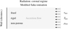 |
Fig. 4 W–Λ simulation setup and boundary conditions. |
3.2 Reference case (W–Λ)
3.2.1 Setup
In the reference case, we simulated the accretion stream using the same physics and assumptions as in previous models (see e.g. Sacco et al. 2008; Koldoba et al. 2008). The matter-radiation coupling is then described by the coronal radiative cooling (Optically thin limit section) and the plasma ionisation was computed with the modified Saha equation (Sect. 2.1.2). In order to simplify the discussion, we focus on the post-shock structure and on the global dynamics. The stellar chromosphere was modelled in the simplest way, hereafter called the “window” model. It consists of a fixed rigid non-porous transparent interface. The main parameters are listed in Fig. 4.
3.2.2 QPO cycle
In addition to the fact that matter accumulates on the left (inner) rigid boundary interface, the system is found to be perfectly periodic. Figure 5 presents five snapshots of density, temperature, and velocity profiles during a QPO cycle far from theinitial stages. The accreted gas falls from right to left. A hot slab of shocked material builds first (t = 2750 and 2884 s) and cools down according to the coronal regime. Below a threshold temperature at which the thermal instability is triggered (~ 8 × 10⁵ K, see Optically thin limit section and references therein for further details), the fast, quasi-isochoric cooling of the slab basis causes the collapse of the post-shock structure (t = 2994 and 3110 s).Just after the full collapse of the slab, a new slab forms and grows (t =3156 s) because the accretion process is still on-going.
This simulation is to be compared to those performed by Sacco et al. (2008); Table 2 lists the main parameters and results for fast comparison. Despite a few key differences (Sun vs. MP Muscæ parameters and “Window” vs. chromospheric heating function), the results agree well.
3.2.3 X-ray luminosity
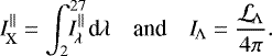
An X-ray radiative power of 1.3 × 1030 erg s−1 was measured in the range 2–27 Å by Brickhouse et al. (2010) for TW Hydræ and an accretion flow velocity estimated at 500 km s−1. We therefore computed the instantaneous X-ray surface luminosity  (in erg cm−2 s−1) and its time average
 (9)
(9)
that are produced by the hot slab, which is here defined by the plasma at temperature above 104.5 K. These luminosities are computed and compared between the different models presented in the subsequent sections and with the observational work of Brickhouse et al. These quantities are commonly compared to the incoming kinetic energy flux. However, the plasma velocity and density may change between the outer boundary of the simulation box and the location of the reverse shock because the flow accelerates in its free-fall from the outer boundary down to the reverse shock. To solve this problem, we must consider the mechanical energy flux. This flux is calculated at any position r by
 (10)
(10)
where the origin of the gravitational energy potential is set at the mean forward-shock position (r0 ≃ 103 km). The conservation of the mechanical energy induces that FM does not depend on the position r. The value derived fromour simulations is FM = 4.2 × 10⁹ erg cm−2 s−1.
Figure 6 shows the time variation of  . As expected, this quantity increases during the propagation of the reverse shock and decreases during the collapse. The time-averaged luminosity
  is equal to 1.5 × 10⁹ erg cm−2 s−1, which corresponds to 36% of the incoming mechanical energy flux FM.
3.3 Effect of a dynamical chromosphere (Chr–Λ)
3.3.1 Setup
In this second setup (see Fig. 7), we aim at studying the effect of a dynamically heated chromosphere on the phenomenon described in the previous section. To achieve this, we divided the computational domain into two zones separated by a Lagrangian interface. Although the column plasma is expected to be at coronal regime, LTE radiation transfer is needed to build the chromosphere layer: it is essential to allow radiation to escape from the first zone through the second (optically thin) zone and this interface must therefore be transparent.
The outer zone was described as before with modified Saha ionisation and optically thin radiative cooling (coronal regime). However, the inner zone was now described by our chromospheric model (see Appendix B). Ionisation was still described by the modified Saha equation, but we used the LTE radiation source terms as given in Eq. (4). To achieve a dynamically heated chromosphere, we first computed a radiative-hydrostatic equilibrium, with the outer zone inactive and with one solar luminosity crossing the entire domain (no effect on the outer zone). Acoustic energy was then injected in the form of monochromatic sinusoidal motion of the first interface (a “Window”) with a 60 s period to mimic solar granulation. Several snapshots of temperature profiles are presented in Fig. B.1. When the shock-heated chromosphere reached its stationary regime, the accretion process was launched (in the outer zone).
3.3.2 Acoustic perturbations
Figure 8 shows seven snapshots of density and temperature profiles during the first QPO cycle (1–354 s). They are followed in the second line by five snapshots of the second QPO cycle (354–415 s). The second cycle differs from the first only during the slab build-up (354–397 s). The sixth snapshot (415 s) is very close to the snapshot of the first cycle at t = 71 s. The (unchanged)end of the second cycle is therefore not reported.
During the installation phase (1–336 s) of the reverse shock, the post-shock structure more or less follows the same scenario as for the reference case (W–Λ). After several periods of the acoustic waves, small differences occur. The reflection and transmission of these waves or shocks to the accretion column depends on the leap of the acoustic impedance between the upper chromosphere and the hot slab. The smallest leap is reached at the end of the collapse, near 336 s, leading to an increase in transmission, which still remains low, however. Their effect leads to small perturbations in the post-shock density (as can already be seen at 168 s).
After this time, the transmitted waves start to feed the hot collapsing layer behind the reverse shock with matter. The thickness of this layer increases, as is shown in Fig. 8 at 351 s, compared for instance with our reference case (3110 s, Fig. 5). This structure collapses and hits the dense chromosphere at 354 s, leading to a secondary reverse shock that propagates backwards inside the slab. This behaviour is confirmed by the velocity variations shown in grey in Fig. 8. The two reverse shocks then pass each other: the positions of the new shock (or contact discontinuity) and the previous(old) one are listed in Table 3. The end of one cycle therefore overlaps the beginning of a new one.
 |
Fig. 5 Lin-log (top) and log-log (bottom) snapshots of the density (green), temperature (red) and velocity (grey) profiles of a QPO cycle (square brackets) with the “W–Λ” setup; the accreted gas falls from the right to the left (adapted from de Sá et al. 2014). From left to right: beginning of a new cycle (t = 2750 s), growth of a hot slab of shocked material (t = 2884 s), quasi-isochoric cooling at the slab basis (thermal instability, t = 2994 s), collapse of the post-shock structure (falling back of the reverse shock, t = 3110 s) and end of the collapse (t = 3156 s). |
Comparison between our reference case (W–Λ) and results obtained by Sacco et al. (2008).
 |
Fig. 6 Time variation of the surface luminosity |

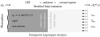 |
Fig. 7 Chr–Λ simulation setup and boundary conditions. A = 0.6575 km s−1 and τ = 60 s. |
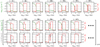 |
Fig. 8 Snapshots of the density (green), temperature (red), and gas velocity (grey) profiles of the first QPO cycle with the Chr–Λ setup; the accreted gas falls from the right to the left. The first line (between 1 and 353 s) corresponds to the first cycle. The second and third lines correspond to the beginning of the second cycle. Snapshots att = 71 s and 415 s arevery close: from this time, the cycle behaves like the previous one. A typical sequence is: growth of a hot slab of shocked material (t = 21 s), quasi-isochoric cooling at the slab basis (thermal instability, t = 168 s), start of the collapse of the post-shock structure (t = 336 s), impact of the collapsing material on the chromosphere (t = 354 s), launch of a new shock before the end of the collapse (t = 358 s), passing of the two shocks (t = 380 s), end of the collapse of the old structure (t = 386 s) and growth of the new slab (t = 415 s). |
3.3.3 Observational consequences
This model implies two main observational consequences. First, compared to the reference case, the QPO cycle period is modified by the acoustic heating. The question of possible resonance is pointless regarding multi-mode acoustic heating by out-of-phase waves emitted in different locations. The period τcycle is slightly reduced (from 400 s for the W–Λ model to 350 s here, Table 1) when solar chromospheric parameters are used. Because the atmospheres of CTTSs have a stronger activity than the solar atmosphere (which we use for the chromospheric model), the effect is expected to be enhanced in CTTSs.
The second effect deals with the X-ray luminosity variation during a cycle, as reported in green in Fig. 6. The growth phase is comparable with the W–Λ setup, but the acoustic perturbations from the chromosphere induce strong differences in the collapse phase. Moreover, the overlapping of the beginning and end of the cycles affects the X-ray luminosity, and the overall amplitude of the variations (contrast) is reduced compared to the reference case. QPO observations may thus require both higher time resolution and improved sensitivity. The time-averaged surface luminosity (Eq. (9)) is here equal to 4.0 × 10⁹ erg cm−2 s−1, namely 94% of the mechanical energy flux FM.
These results show that compared to the reference case, the dynamical heating of the chromosphere affects the duration of the QPO period and its observability. Of course, a more realistic description of the chromospheric heating would require at least a 2D magnetohydrodynamical (MHD) picture. For instance, we know that chromospheric perturbations inside the column may lead to the development of fibrils (see e.g. Matsakos et al. 2013, ChrFlx# models), which is one of the scenarii explaining the absence of observation of QPO. In the acoustic description of the chromospheric heating, these fibrils, evolving out of phase, will also be strongly affected by the chromospheric perturbations.
3.4 Radiation effect on accretion (Hybrid)
3.4.1 Setup
In this section, the plasma model includes collisional-radiative ionisation (see Sect. 2.1.2). The radiation-matter coupling is described within the intermediate regime (see Intermediate regimes section) and the outer radiation flux is set to  . The goal of this last setup (see Fig. 9) is to inspect the net effect of the matter-radiation coupling. We therefore chose not to consider any chromospheric activity. Following the preliminary process of the previous setup (see Sect. 3.3.1), the outer zone gas was first fixed in place and the radiative hydrostatic equilibrium was computed in the inner zone. However, this outer zone was radiatively heated by the chromosphere up to 5730 K. When the stationary regime was reached, the accretion process was launched. A key advantage of this process is that nothing is needed to maintain the chromospheric structure, which can therefore freely evolve depending on the physical processes in play alone.
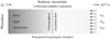 |
Fig. 9 Hybrid simulation setup and boundary conditions. |
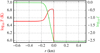 |
Fig. 10 Electron ionisation rate ( |
3.4.2 Ionisation model
We tested in this setup the effect of the time-dependent ionisation through radiative ionisation, radiative recombination and collisional ionisation with a time-dependent formulation (see Sect. 2.1.2 for more details). The main difference brought by a time-dependent calculation of the electron density is a tiny ionisation delay behind the reverse shock front, as shown in Fig. 10.
At the shock front, the kinetic energy is converted into thermal energy, and then a part of this thermal energy is used to ionise the post-shock material with a timescale connected to the ionisation rates; the affected gas layer is up to 0.2 km thick and thus negligible compared to the whole structure (which is at least 104 km thick, see Table 1). This justifies the use of a time-independent model for ionisation in the previous setups (W–Λ and Chr–Λ). Günther et al. (2007) and Sacco et al. (2008) obtained the same conclusion from different approaches.
However, compared to the Saha–Brown equilibrium calculations, the use of collisional and radiative rates to derive the equilibrium electron density brings differences in the transition between the (almost) neutral medium and the fully ionised plasma. This transition lies between 103.6 and 104.2 K. However, such temperatures are only reached by the accreted gas during the cooling instability. Its overall effect is hence negligible. The results presented for the Hybrid case (see Fig. 11) are thus based on this collisional-radiative equilibrium calculation of ne.
3.4.3 Radiation and ionisation feedback
The first cycle is presented in Fig. 11; it shows the time variations over 160 s of the gas temperature and mass density, of the photon escape (ζ) and absorption (1− ζ) probabilities, and of the radiation energy volumetric density and flux (Er and Fr) (see Intermediate regimes section) for the same snapshots. The next cycles only differ from this first one by the position of the interface between the slab and the chromosphere, as discussed in Pre-heating of the accretion flow section.
The global behaviour follows the trends of the two previous models. However, several effects must be highlighted: a heating of the chromosphere and of the accretion flow, already pointed out by Calvet & Gullbring (1998) and Costa et al. (2017), and the reduction of the oscillation period and of the post-shock extension. These effects are discussed below.
 |
Fig. 11 Snapshots of the mass density (green), gas temperature (red), escape ζ (dark blue) and absorption probabilities 1−ζ (cyan, see Intermediate regimes section), velocity (grey), electron density (light green), radiation energy density (magenta), and flux (orange) profiles of the first QPO cycle with the Hybrid setup. The accreted gas falls from the right to the left on an equilibrium atmosphere. |
 |
Fig. 12 Position of the reverse shock (rrev, purple) and the corresponding velocity (vrev, grey) together with the accreted plasma temperature before the hot slab (Tacc, dark gold) and the upper chromosphere temperature (Tchr, red) for the first QPO cycle in the Hybrid case. |
QPO cycle reduction
Although 1−ζ shows strong variations, its net value beyond the forward shock remains negligible and the post-shock material is within the coronal limit (as in Sect. 3.2). The temperature behind the reverse shock is here equal to 3.1 × 10⁶ K, to be compared to4 × 106 K in the reference case. In addition, the compression is enhanced from 4 (W–Λ case) to 4.4. As a consequence, the cooling is more efficient: the cooling time is reduced from 400 s down to 220 s, which is compatible with the duration of the cycles. This effect is due to the ionisation and recombination energy cost (qχ), which is included in the gas energy equation for the Hybrid case, but not for the reference case (qχ = 0 in W–Λ case, see Eq. (1) and Sect. 2.1.2).
Radiation energy and flux
The radiation energy density increases between 9 s and 100 s, which corresponds to the growth phase of the hot slab. This increase is however correlated to the upper chromosphere heated up to 12 000 K (discussed in section Chromospheric heating and beating and presented Fig. 12). Er remains almost flat in the optically thin post-shock medium, with a value driven by the heated upper chromosphere. In the accretion flow, during the growth of the hot slab, there is a tiny decrease due to the absorption by the accreted material up to 0.5% at 70 s (see Pre-heating of the accretion flow section).
The radiative properties of the inner chromosphere is well described by the diffusive limit: Er ≃ aR T4 and Fr ≃ cEr∕4. The most peculiar feature of the radiative flux is its linear growth through the post-shock slab. This pattern is characteristic of a volume emission by an optically thin medium. As discussed before, the radiative energy in the hot slab is somewhat imposed by the heated upper chromosphere: as a consequence, the outgoing radiation flux is  , with Tchr the temperature of the upper chromosphere (Fig. 12). Then, the radiation flux propagates through the accretion flow with negligible changes.
Because Fr is counted negatively towards the star, the flux emitted by the slab is offset by the flux produced by the chromosphere. The net radiation flux then rises back into the chromosphere.
However, the variations of Fr within the slab come from the interweaving of several radiation sources (the chromosphere, the slab itself, and the accretion flow): these variations must be interpreted with care knowing the limitations of the M1 model (see Sect. 2.2.2).
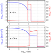 |
Fig. 13 Snapshots of the temperature (red) and pressure (blue) at 9 s (top) and 70 s (bottom) for the Hybrid case. |
Chromospheric heating and beating
The upper chromosphere is heated by the radiating post-shock plasma to up to 12 000 K (Fig. 12). For instance, between 9 and 70 s, its temperature varies from 7000 to 10 800 K at 800 km and the pressure increases from 800 to 2600 dyn cm−2 at this location (Fig. 13). As a consequence, the whole post-shock structure is pushed upwards from 875 to 3150 km, that is, out of the unperturbed chromosphere (by about 2000 km, see e.g. Vernazza et al. 1973).
At the end of the cycle, the chromosphere is no longer heated and the slab sinks back into the atmosphere. The expected behaviour isan oscillation of the slab depth with the same periodicity as QPOs because it originates from the hot post-shock plasma radiation. At the end of this first cycle, the chromosphere does not recover its initial thickness: this effect does not affect the post-shock dynamics and cycle characteristics. All these effects are overestimated in a 1D model. However, this study shows that the general question of the slab depth, which is important for X-ray observations, can only be addressed within a model that takes the radiative heating of the chromosphere by the hot slab into account.
Pre-heating of the accretion flow
When itreaches the hydro-radiative steady state of the chromosphere, the flow has been homogeneously heated from 3000 to 5730 K before the start of the accretion process. During the cycle, the accretion leads to an additional heating of the flow up to ~ 8500 K (at t = 93 s). These effects are quantified in Fig. 12, which reports the time variations of the position and velocity of the interface between the hot slab and the accretion flow, as well as the temperatures of the heated chromosphere and of the pre-shock material. The use of the escape probability formalism (see Intermediate regimes section) induces a dependence of the absorption by the accretion flow with the section of the column; changing this section from 1000 to 10 000 km, for instance, will vary the parameter ζ from 1− 5 × 10⁻³ to 1− 5 × 10⁻²; this increases the absorption and thus the radiative heating of the pre-shock flow.
Such preheating has been pointed out by other authors (Calvet & Gullbring 1998; Costa et al. 2017). In these works, this heating is induced by radiation from the hot slab through photo-ionisation. Although radiative cooling of the accretion flow may be included in some cases, the radiation transfer is not taken into account. Depending on the conditions, the pre-shock temperature may reach from 20 000 K (in CG98) up to 105 K (in Co17) close to the reverse shock (up to 104 km). In the latter, this precursor is preceded by a flatter and cooler (~ 104 K) zone with an extension of 105 km, which is smaller than ours (> 105 km).
Our simulation shows that part of the heating is a consequence of the chromospheric radiation that is in play before the start of the accretion. The analysis of the variation of the radiative energy indicates that additional heating operates during the development of the hot slab. However, as we do not include any dependence on the wavelength, it remains very difficult to distinguish in detail the role played by the radiation that is emitted by the hot slab (X-rays) and from the (heated) chromosphere (UV-visible). Complementary information will be given by the synthetic spectra that were computed as a post-process of the hydrodynamics structures (Sect. 3.4.4).
X-ray luminosity
The X-ray luminosity of the system is computed following the method described in Sect. 3.2.3. Its time variation (in units of τcycle = 160 s) is reported in Fig. 6 for comparison with the two previous cases. Compared to the reference case, in addition with a shortening of the period, this case presents a more pronounced radiative collapse (70–90 s), followed by a chaotic collapse (90–160 s). The time average of the radiative surface luminosity here is equal to 1.2 × 10⁹ erg cm−2 s−1, which represents 30% of the mechanical energy flux (Fig. 6).
3.4.4 SYNSPEC monochromatic emergent intensity
Because thissimulation is performed using only one group of radiation frequencies, it is interesting to analyse the details of the previous radiative heating via its feedback on the monochromatic emergent intensity more precisely.
To this purpose, the hydrodynamic structures were post-processed with the SYNSPEC code (Sect. 2.3.3). For consistency purposes, we took the atomic data that were used to calculate the average opacities (see Sect. 2.2.3 and Appendix A). We therefore estimated the specific intensity  (in erg cm−2 s−1 Å−1 sr−1) along the direction of the column. Because the line profile behaviour is not investigated here, velocity effects are neglected.
It is important to recall that a quantitative comparison of this synthetic spectrum with observations, especially inthe X-rays (see e.g. Güdel et al. 2007; Robrade & Schmitt 2007; Drake et al. 2009), would require NLTE and 3D radiative transfer post-processing. Nonetheless, using 1D radiative transfer and the LTE approximation is interesting here because it corroborates or refutes the generally accepted trends, such as a strong X-ray emission and an excess of luminosity in the UV-VIS range (Calvet & Gullbring 1998; Brickhouse et al. 2010; Ingleby et al. 2013).
A typical spectrum emerging from 4.6 × 10⁴ km (located within the accretion flow) is reported in Fig. 15). It was computed from a snapshot (t =70 s) of the Hybrid model (see Figs. 11 and 14). At this stage, the chromosphere extends up to 1.4 × 10³ km, the hot plasma from1.4 × 103 to 8.3 × 10³ km, and the accretion flow from 8.3 × 10³ to 1 × 10⁵ km. The intensity that emerges from this layer presents three characteristic spectral bands:
-
in the range 1–100 Å (X-rays), the bump is attributed to the hot post-shock plasma, with intense lines up to 102 erg cm−2 s−1 Å−1;
-
in the range 100–900 Å (EUV), radiation is efficiently absorbed by the inflow;
-
in the range 900–10 000 Å (UV+Vis+IR), the second bump is attributed to the heated stellar chromosphere and photosphere (a black body at T ≃ 11 300 K, see Fig. 12).
The strong absorption of the EUV radiation is due to the huge optical depth of the accretion flow at ρ = 10−13 g cm−3 and T ≃ 5000−8000 K. This effect may then be attenuated in the case of a bent column or when the observation is performed side-on and not along the column. This absorption effect on the spectrum is illustrated in Fig. 16, which presents the intensity emerging right after the reverse shock front, at r = 8.3 × 10³ km. This figure shows that this absorption to a lesser degree also affects the visible spectrum originating from the chromosphere. This must be considered when interpreting the UV excess (see e.g. Calvet & Gullbring 1998; Hartmann et al. 2016; Colombo et al. 2019). We also expect a pre-heating of the accretion flow as a result of the EUV absorption. Such pre-heating is also obtained independently by AstroLabE (Pre-heating of the accretion flow, section); however, a one-to-one correspondence would require a multi-group description of the radiation field in AstroLabE.
We compute from  (Fig. 14) the net X-ray outgoing intensity (
 ) and the corresponding coronal quantity (IΛ):
 (11)
(11)
The time variations of these two quantities, reported in Fig. 17, present similar characteristics. However, the values derived by SYNSPEC are higher by about two to three orders of magnitude. This discrepancy is either imputable to the LTE approximation or to the assumed 1D plane-parallel geometry. Our synthetic spectra therefore cannot be used for a quantitativecomparison with observations.
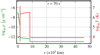 |
Fig. 14 Snapshot of the density (green) and temperature (red) profiles at t = 70 s with the Hybrid setup, post-processed hereafter. |
 |
Fig. 15 Specific intensity |

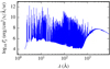 |
Fig. 16 Specific intensity |

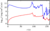 |
Fig. 17 Time-variation of the 2–27 Å (LTE) integrated X-ray outgoing intensity ( |

4 Refining the models
4.1 More realistic chromosphere
It should be pointed out that we used a solar model for the chromosphere with acoustic heating. Compared to the description of this heating, a more important improvement would be to consider a realistic T Tauri chromospheric model, which is currently not very well known. This may affect the ionisation (and then gas pressure with another chemical abundances) as well as slab characteristics (through gravity) and radiation effects (through opacities and incoming luminosity). Our results are therefore to be considered qualitatively and not quantitatively.
4.2 Improvements of the radiation model
We used radiation momenta equations with the M1 closure relation. Although this is already a strong improvement compared to other approaches like the diffusion model, it could be improved by using radiation half-fluxes (e.g. the inward an outward components of the radiation flux). This should separate the radiation flux from the star and from the post-shock structure.
The M1 closure relation allows the radiation field to reach at most one direction of anisotropy; half-fluxes can extend it to two, which is the maximum number of anisotropy directions reachable in 1D. Half-fluxes (along with M1) would then be equivalent to the momenta equations with the M2 closure relation (Feugeas 2004), without its prohibitive numerical cost.
The M1 model and its limits have been thoroughly studied (see e.g. Levermore 1996; Dubroca & Feugeas 1999; Feugeas 2004). The behaviour of this model in combination with half-fluxes still needs to be examined, however.
Concerning the opacity averages, this work is performed within the monogroup approach: the intergrated Planck and Rosseland opacities are obtained supposing that the whole spectrum follows more or less a black-body profile. However, the spectra we computed as emerging from accretion structures are expected to present three discernible frequency groups:
-
up to the visible domain, the spectrum is dominated by the black body emerging from the stellar photosphere;
-
the EUV band is expected to be depleted due to high absorption by the accreted gas;
-
the X-ray band is thought to be optically thin and to include the hot-slab signature.
Although the multi-group approach is numerically more challenging, it will improve the study of the consequences of the radiation absorption by the surrounding medium. A consequence of the X-ray and EUV absorption by the cold accretion flow is the presence of a radiative precursor. Such a phenomenon cannot be obtained through a monogroup approach. Moreover, a three-group approach will provide a better description of the feedback of the hot slab on the stellar chromosphere.
4.3 NLTE effects in radiation hydrodynamics and in synthetic spectra
Two other points may be improved. First, the transition model (ζ) remains qualitative and may need to be extended to the ionisation calculation. The work done by Carlsson & Leenaarts (2012) offers paths to reach this consistency and may need to be investigated further. A better model of the LTE transfer, line cooling, andintermediate regimes may demand dedicated NLTE opacities, namely plasma emissivity (equivalent to ne nH Λ), radiation energy absorption (κP), and radiation flux sinking (κR). Moreover, all these quantities, computed with a radiative-collisional model, have to be averaged over adequate weighting functions. Based on recent progress in this topic (Rodríguez et al. 2018), new results are expected in the near future. Independently, an NLTE description should be used to compute the emerging spectra: this work is already in progress using the TLUSTY code.
5 Conclusion
We used 1D simulations with detailed physics to determine the validity of the two following common assumptions in accretion shock simulations: the stellar atmosphere can either be modelled by a hydrostatic or a steady hydrodynamic structure, and the dynamics of accretion shocks is governed by optically thin radiation transfer. We first verified that we are able to recover previous results (Sacco et al. 2008, W–Λ case, Sect. 3.2) and independently tested each of these assumptions (Chr–Λ case, Sect. 3.3, and Hybrid case, Sect. 3.4). Each of them proves to have a non-negligible effect on the typical characteristics of the accretion dynamics and on the estimation of its X-ray surface luminosity. This one varies between 1 and 4 × 10⁹ erg cm−2 s−1. Taking the radiative power of Brickhouse et al. (2010) as a reference, we derived a section of the accretion spot from 3 × 10²⁰ to 1 × 1021 cm2, corresponding to a filling factor of the solar disc between 2 and 8%, namely a stream composed of ~104 fibrils of radius Lc (see Sect. 3.1) or a column of radius 100 × Lc, assuming that the global dynamics of the system is not influenced by this larger section of the column through radiative effects.
In the case of the chromosphere, which is heated by acoustic perturbations that degenerate into small shock waves, we showed that these perturbations do not strongly modify the cycle period compared to the reference case. However, the cycle becomes chaotic due to the generation of secondary shock waves. As a result, the relative duration of the hot phase in the cycle remains longer and thus the variability in the X-rays is less pronounced than for the reference case. To be detected, it would require a better sensitivity of the photometric measurements.
In the case of an initially steady atmosphere at radiative equilibrium, the coupling between the radiation and the hydrodynamics leads to three major effects. First, the incoming flow is radiatively pre-heated over the length of the simulation box. Second, the chromosphere successively expands and retracts as a result of the radiative feedback (heating) on it; this in particular pushes the column up, which is favourable to the lateral escape of the X-ray emitted from the hot slab. Third, a chaotic radiative collapse affects the time variation of the X-ray flux (Fig. 6). Moreover, the inclusion of ionisation in the energy balance leads to non-negligible effects in the post-shock temperature that modify the cooling efficiency and therefore the cycle duration.
In this hybrid case, we computed at LTE the radiative intensity emerging from the location of the reverse shock (Fig. 15) as also from the outer boundary (Fig. 16). The flux is characterised by a huge number of atomic lines in the X rays, and follows a black-body profile in the visible, with the presence of emission and absorption lines, and third by an EUV component that is very strong at the position of the reverse shock and disappears at the outer boundary as a result of thestrong absorption.
This study could be followed by a more complete simulation that would include both a dynamically heated chromosphere and the hybrid setup. However, it appears at this stage more important to take an NLTE radiative description based on adapted opacities and radiative power losses into account. Another necessary improvement will be through a multi-group radiation transfer to catch at least the effect of the EUV absorption and X-ray radiative losses on the structure of the column, and to analyse the possibility of a radiative precursor that could pre-heat the incoming flow. The study is also to be extended to multi-dimensional simulations to determine the effects of both radiation and magnetic field closer to the real picture (Orlando et al. 2010, 2013; Matsakos et al. 2013, 2014).
Acknowledgements
We express our gratitude to Jason Ferguson for providing us with the molecular LTE opacity tables we used, and toFranck Delahaye for his contribution to the atomic LTE ionisation data we used for both the opacity tables and for the radiative transfer post-processing. We thank Rafael Rodriguez for sharing helpful preliminary results about NLTE microscopic collisional-radiative data, Salvatore Orlando for reading the manuscript, Ziane Izri for his contribution at the beginning of this project, andChristophe Sauty for helpful discussions. I.H. thanks the Physics Department of Sorbonne Université for his visiting professorship. This work was supported by the French ANR StarShock and LabEx Plas@Par projects (resp. ANR–08–BLAN–0263–07 and ANR–11–IDEX–0004–02), PICS 6838, Programme National de Physique Stellaire of CNRS/INSU and Observatoire de Paris.
Appendix A Opacity tables
The specificity of the accretion shock study led us to work on dedicated opacity tables. We detail in the appendix the reasons behind this choice and the creation process. The resulting opacity table is accessible upon request.
A.1 Motivation
Most available opacity tables are defined in a slanted (ρ, T) or (ne, T) domain (like in Fig. A.1). However, one peculiarity of accretion shock structures is the low-density hot post-shock plasma (black curve vertex in Fig. A.1) that explores a domain that is not covered by publicly available tables. More complete tables are thus mandatory for our study.
A.2 Choice of primary tables
To cover the density and temperature range corresponding to our conditions, we implemented in the code SYNSPEC (see Sect. 2.3.3), which initially was dedicated to stellar atmospheres, modules that allowed us to generate LTE monochromatic opacities at a given density and temperature. These monochromatic opacities were then averaged with the proper weighting functions to generate the adequate Rosseland and Planck mean opacity tables (hereafter called SYNSPEC tables, see Fig. A.2, top panels). These opacities are consistent with those from the Opacity Project (see e.g. Opacity Project Team 1995), which we use as reference, for T between 103.5 and 107.5 K. The advantage of SYNSPEC comes from the high number of atomic species considered because a very detailed chemical composition is necessary to model the radiation properties of a plasma at high temperatures.
However, below 103.5 K, the molecular chemistry cannot be neglected, but is not included in this work on SYNSPEC. We therefore completed the SYNSPEC tables with low-temperature molecular opacities provided by Ferguson et al. (2005) between 103 and 104 K (Ferguson tables, see Fig. A.2, bottom panels), which show excellent agreement with those from the Opacity Project at upper temperatures. To facilitate the merging process, we obtained from the authors tables with compatible density and temperature grids (Ferguson, priv. comm.): the mesh points from the Ferguson and SYNSPEC tables are identical in the common domain (103.5−104 K and 10−14−10−6 g cm−3).
A.3 Preliminary study
A.3.1 Analysis of primary tables
Considering opacity variations as well as temperature and density ranges, we decided to work with the logarithm of all these quantities. As first derivatives, we used
![Mathematical equation: \begin{equation*}\left\{\!\!\begin{array}{l@{\,}c@{\,}c@{\,}c@{\,}c@{}c} \partial_{lT}l\kappa &=& \dfrac{\partial\log_{10}\kappa}{\partial\log_{10}T} &=& \dfrac{T}{\kappa}&\dfrac{\partial\kappa}{\partial T},\\[13pt] \partial_{l\rho}l\kappa &=& \dfrac{\partial\log_{10}\kappa}{\partial\log_{10}\rho} &=& \dfrac{\rho}{\kappa}&\dfrac{\partial\kappa}{\partial\rho}, \end{array}\right. \end{equation*}](/articles/aa/full_html/2019/10/aa33400-18/aa33400-18-eq30.png) (A.1)
(A.1)
where κ stands for κP or κR.
Preliminary analysis of SYNSPEC and Ferguson tables revealed local aberrations, especially in the temperature or density derivatives (see Fig. A.3). We may use the merging process to smooth most aberrations.
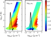 |
Fig. A.1 Planck (left) and Rosseland (right) opacities (in cm2 g−1) with respect to gas density and temperature in log scale, as provided by the Opacity Project (Opacity Project Team 1995). The black curve is a typical characteristic of an accretion column. |
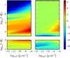 |
Fig. A.2 SYNSPEC (top) and Ferguson (bottom) Planck (left) and Rosseland (right) opacities (in cm2 g−1) with respectto gas density and temperature in log scale. The dotted lines show transition temperatures chosen for each table (see Appendix A.4.1). |
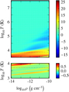 |
Fig. A.3 ∂lTlκR from SYNSPEC table (top) and ∂lρlκP from Ferguson table (bottom) with respect to the logarithm of gas density and temperature. The dotted lines show the transition temperatures chosen for each table. Some anomalies are revealed, especially around 103.7 K and high densities: this zone is cut during the merging process. |
A.3.2 Physical and numerical constraints
In order to obtain a satisfying merging, several numerical and physical constraints must be respected. First, opacities must as far as possible be of class C1 (values and first derivatives must be continuous). Then, the transition region should be as narrow as possible. Finally, the transition region must encompass the anomalies that are encountered in both primary tables.
Such a table is composed of a limited number of discrete points: the first constraint can be reported to the interpolation method as far as opacity values in the transition present smooth variations. To ensure a smooth transition between the molecular and the atomic (primary) tables, the transition must not take the values within the transition into account. The transition values therefore loose any physical meaning and must be as few as possible. We note that the Ferguson tables showed opacity discontinuities in their hottest and densest part, as did SYNSPEC tables in their coolest and densest part (see Fig. A.3). Because the values within the transition region are ignored, we use it to artificially remove anomalies: as far as possible, the transition region must be chosen so that it covers most of them. We achieve this objective, but a few anomalies remain in regions that are notexplored in our simulations (see Fig. A.4); this problem therefore is postponed for now.
A.4 Merging process
A.4.1 Method
In this section, the index A refers to values taken at the lower transition temperature, and the index B refers to the upper transition temperature. The transition temperatures chosen to merge SYNSPEC and Ferguson tables are
-
TA = 103.71 K and TB = 103.80 K for κP (~1200 K wide);
-
TA = 103.65 K and TB = 103.86 K for κR (~2800 K wide).
The problem is decoupled in temperature and in density. First, we considered the merging at each mesh density as an isolated problem. Then, we applied a correction (if needed) to improve the smoothness along the density.
A.4.2 Merging along the temperature
To satisfy the class C1 constraint, we used piecewise cubic Hermite polynomials, which ensure continuity of values (κA, κB) and derivatives (∂lT lκA, ∂lTlκB) at each transition limit. The partial derivatives (∂lTlκA and ∂lTlκB) are based on van Leer (1973) slopes, to prevent the apparition of spurious extrema in forcing their location to the estimated closest mesh point. This method can be found for instance in Auer (2003) and Ibgui et al. (2013) (the Fritsch & Butland 1984 derivatives used in these papers generalise van Leer slopes to non-regular grids).
For eachgrid density ρj, the opacity at temperature Ti ∈ [TA, TB] was estimated using the formula
![Mathematical equation: \begin{equation*} \begin{array}[b]{@{}r@{}l@{}} \log_{10}\kappa(T_{\!i};\!\rho_{\!j}) = u_i^2\,(3-2u_i)\,\log_{10}\kappa_{\mathrm{B}} &\,+\, (u_i-1)\hphantom{^2}u_i^2\,h\;\partial_{lT}l\kappa_{\mathrm{B}}\\[4pt] +\, (u_i-1)^2\,(2u_i+1)\,\log_{10}\kappa_{\mathrm{A}} &+(u_i-1)^2\,u_i\,h\;\partial_{lT}l\kappa_{\mathrm{A}},\hspace{-1em}\null \end{array} \end{equation*}](/articles/aa/full_html/2019/10/aa33400-18/aa33400-18-eq31.png) (A.2)
(A.2)
with h = log10TB − log10TA and ui = (log10Ti − log10TA)∕h. This expression can be rewritten as a third-degree polynomial in ui.
A.4.3 Density correction
At this stage, we reached class C1 along the temperature, but there is no guarantee of continuity along the density. However, in practice, it was C1, except for few mesh temperatures  .
.
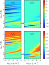 |
Fig. A.4 Merged table Planck (left) and Rosseland (right) opacity temperature (top) and density (bottom) first derivatives in the (ρ,T) plane, in logscale; the grey shape represents the transition region. |
Because the dependency in density is held by the third-degree polynomial coefficients, we considered the behaviour of each of them with respect to density. Every coefficient showed spurious variations only at densities  . We therefore applied piecewise cubic Hermite polynomials along with van Leer (1973) slopes (density derivatives) to estimate these coefficients for each
  . These new coefficients were then used to re-estimate the opacity values along the temperature for the
  .
.
A.4.4 Final tables and interpolation process
We verified the smoothness of the result through the behaviour of the first partial derivatives. Figure A.4 shows no anomaly within the transition temperature range [TA, TB] (grey shape). The remaining anomalies are not reached in our simulations.
The interpolation process was copied from the merging method (piecewise cubic Hermite polynomials along with van Leer slopes) because it satisfies the criteria described in Appendix A.3.2. Interpolation was first performed along the temperature at the 2 × 2 grid densities framing the requested density to calculate van Leer slopes at the requested temperature and interpolate along density.
Interpolating along the temperature and then density showed to be slightly more accurate than interpolation along the density first. This is arguably due to stronger variations of the opacities (especially the Planck mean opacity) with respect to temperature.
Appendix B Chromospheric model
One of our objectives is to describe the dynamics of the column and its effect on the chromosphere, as well as the feedback of the chromosphere on the column. This requires including an adequate description of the physical mechanism that leads to the chromospheric heating. This appendix presents the simple but self-consistent model of the chromosphere we used.
B.1 Motivations and limits
The study of the solar chromosphere is a tough problem in itself. Modelling the solar chromosphere is of interest for us because the base of the accretion column lies in the stellar chromosphere: the dynamics and observability of the column base may therefore depend on its structure and dynamics. Moreover, the chromosphere may be heated locally by the accretion process. The inner heating mechanism in the chromosphere is still subject of debate: it is mainly thought to originate either from acoustic wave dissipation (Biermann 1946; Schwarzschild 1948; or more recently Sobotka et al. 2016) or from MHD wave dissipation (Alfvén & Lindblad 1947; Jess et al. 2015).
Most accretion simulations model the stellar atmosphere (when it is modelled) as a hydrostatic plasma layer that is tuned up with ad hoc sources to recover both temperature and pressure profiles (see e.g. the heating function empirically introduced by Peres et al. 1982). Although this must work for a static structure, it is delicate to predict the dynamic behaviour of such a structure when it faces the continuous perturbation from an infalling plasma flow: this solution is not adapted to studies involving (in a self-consistent way) the dynamics of a perturbed atmosphere, like in the context of accretion.
We do not pretend to develop a complete modern model in this paper: we only aim at using a reasonable model that is both dynamic and self-consistent with our radiation hydrodynamics model. In our 1D model, we do not consider any magnetic effect but a very effective confinement of the accretion flow along the field lines. To allow fast qualitative comparison between our model and theoretical models and observations (see Fig. B.1), we only used solar parameters (abundances, luminosity, mass, and radius).
B.2 Acoustic waves and shocks
Acoustic waves are generated by photospheric granulation (see e.g. Judge 2006). These waves propagate upwards up to the height where their velocity overcomes the local sound speed, and then degenerate into shocks. The nature of this mechanism is random: two different locations at the stellar surface are crossed over by acoustic shocks that ought to be out of phase with each other.
In our simulations, acoustic energy is supplied in the form of a monochromatic sinusoidal motion of the first Lagrangian interface (T = 60 s and facc = 108 erg cm−2 s−1, see e.g. Rammacher & Ulmschneider 1992; Ulmschneider et al. 2005; Kalkofen 2007). Resulting acoustic waves propagate and degenerate into shocks. Figure B.1 shows several temperature snapshots of such a simulation along with the chromospheric model from Vernazza et al. (1973). Below 300 km, acoustic waves are damped and barely appear on snapshots. Above 500 km, waves are fully degenerated into shocks: their strength is then governed by the balance between steepening in the pressure gradient and dissipation. Because the corona and the upper chromosphere (above 103 km) are readily crushed by the accretion flow, the heating of these areas is not considered in our model.
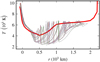 |
Fig. B.1 Successive snapshots of acoustic wave propagation (thin lines) and mean chromospheric temperature (thick red line, Vernazza et al. 1973). The simulation setup is described in Sect. 3.3.1; the solar photosphere is located at r = 0 km. Adapted from Chièze et al. (2012). |
B.3 From the solar to a stellar chromosphere
Observations of the solar chromosphere provide time and space averages of thermodynamics quantities (ρ, T, p, etc.). Detailed observation of CTTS chromospheres would demand higher space and time resolution than is permitted by current observational technologies. Most works on this field therefore rely on scaling laws (see e.g. Ayres 1979; Calvet 1983) or ad hoc fittings to recover specific observational features (see e.g. Dumont et al. 1973; Cram 1979; Calvet et al. 1984; Batalha & Basri 1993).
Appendix C Radiation source terms (Hybrid model)
This work encompasses several radiation regimes, from optically thick LTE radiation transfer (Optically thick limit section) to the optically thin coronal NLTE regime (Optically thin limit section). The momenta equations (Sect. 2.2) can handle all of them, assuming the proper radiation source terms are provided.
In the LTE case, both radiation energy and momentum source terms are well defined (Eq. (4)). In the coronal regime, this is not the case: gas and radiation are decoupled. Radiation therefore only acts as a gas energy sink: the radiation energy source term (the gas sink) is reduced to a cooling function (see for instance Kirienko 1993). Computing the radiation flux is irrelevant in this regime and therefore no radiation momentum source term is provided. That is why we set  to 0.
to 0.
In the Hybrid setup, we aim at modelling radiative conditions that are neither LTE nor coronal regimes, but something in between. To determine whether the situation is closer to one or the other, and how close, we considered the probability for a photon to escape the accretion column (see Eq. (7)). We used it as a weighting factor to average the source terms, as shown in Intermediate regimes section.
The process is straightforward for the radiation energy source term, but not for the radiation momentum source term because  remains unknown. We therefore assumed that the coronal Rosseland mean opacity does not significantly differ from its LTE value. This intuition is reinforced by the recently computed NLTE radiative collisional opacities (Pérez, priv. com. and Rodríguez et al. 2018).
References
- Alfvén, H., & Lindblad, B. 1947, MNRAS, 107, 211 [NASA ADS] [CrossRef] [Google Scholar]
- Argiroffi, C., Maggio, A., & Peres, G. 2007, A&A, 465, L5 [NASA ADS] [CrossRef] [EDP Sciences] [Google Scholar]
- Argiroffi, C., Maggio, A., Peres, G., et al. 2009, A&A, 507, 939 [NASA ADS] [CrossRef] [EDP Sciences] [Google Scholar]
- Auer, L. H. 2003, in Stellar Atmosphere Modeling, ASP Conf Ser., 288, 3 [Google Scholar]
- Ayres, T. R. 1979, ApJ, 228, 509 [NASA ADS] [CrossRef] [Google Scholar]
- Batalha, C. C., & Basri, G. 1993, ApJ, 412, 363 [NASA ADS] [CrossRef] [Google Scholar]
- Biermann, L. 1946, Naturwissenschaften, 33, 118 [NASA ADS] [CrossRef] [Google Scholar]
- Bonito, R., Orlando, S., Argiroffi, C., et al. 2014, ApJ, 795, L34 [Google Scholar]
- Bouquet, S., Stehlé, C., Koenig, M., et al. 2004, Phys. Rev. Lett., 92, 225001 [NASA ADS] [CrossRef] [Google Scholar]
- Bouvier, J., Covino, E., Kovo, O., et al. 1995, A&A, 299, 89 [NASA ADS] [Google Scholar]
- Brickhouse, N. S., Cranmer, S. R., Dupree, A. K., Luna, G. J. M., & Wolk, S. J. 2010, ApJ, 710, 1835 [NASA ADS] [CrossRef] [Google Scholar]
- Brown, J. C. 1973, Sol. Phys., 29, 421 [NASA ADS] [CrossRef] [Google Scholar]
- Calvet, N. 1983, Rev. Mex. Astron. Astrofis., 7, 169 [NASA ADS] [Google Scholar]
- Calvet, N., & Gullbring, E. 1998, ApJ, 509, 802 [NASA ADS] [CrossRef] [Google Scholar]
- Calvet, N., Basri, G., & Kuhi, L. V. 1984, ApJ, 277, 725 [NASA ADS] [CrossRef] [Google Scholar]
- Carlsson, M., & Leenaarts, J. 2012, A&A, 539, A39 [NASA ADS] [CrossRef] [EDP Sciences] [Google Scholar]
- Charignon, C., & Chièze, J.-P. 2013, A&A, 550, A105 [NASA ADS] [CrossRef] [EDP Sciences] [Google Scholar]
- Chevalier, R. A., & Imamura, J. N. 1982, ApJ, 261, 543 [NASA ADS] [CrossRef] [Google Scholar]
- Chièze, J.-P., de Sá, L., & Stehlé, C. 2012, EAS Pub. Ser., 58, 143 [CrossRef] [Google Scholar]
- Colombo, S., Orlando, S., Peres, G., Argiroffi, C., & Reale, F. 2016, A&A, 594, A93 [NASA ADS] [CrossRef] [EDP Sciences] [Google Scholar]
- Colombo, S., Ibgui, L., Orlando, S., et al. 2019, A&A, accepted [Google Scholar]
- Costa, G., Orlando, S., Peres, G., Argiroffi, C., & Bonito, R. 2017, A&A, 597, A1 [NASA ADS] [CrossRef] [EDP Sciences] [Google Scholar]
- Cram, L. E. 1979, ApJ, 234, 949 [NASA ADS] [CrossRef] [Google Scholar]
- Curran, R. L., Argiroffi, C., Sacco, G. G., et al. 2011, A&A, 526, A104 [NASA ADS] [CrossRef] [EDP Sciences] [Google Scholar]
- de Sá, L. 2014, PhD Thesis, Université de Paris VI, Paris, France [Google Scholar]
- de Sá, L., Chièze, J.-P., Stehlé, C., et al. 2012, in SF2A-2012: Proceedings of the Annual meeting of the French Society of Astronomy and Astrophysics, eds. S. Boissier, P. de Laverny, N. Nardetto, et al., 309 [Google Scholar]
- de Sá, L., Chièze, J.-P., Stehlé, C., et al. 2014, Eur. Phys. J. Web Conf., 64, 04002 [CrossRef] [Google Scholar]
- Dorfi, E. A., & Drury, L. O. 1987, J. Comput. Phys., 69, 175 [NASA ADS] [CrossRef] [Google Scholar]
- Drake, J. J. 2005, in 13th Cambridge Workshop on Cool Stars, Stellar Systems and the Sun (Paris: European Space Agency), 519 [Google Scholar]
- Drake, J. J., Ratzlaff, P. W., Laming, J. M., & Raymond, J. C. 2009, ApJ, 703, 1224 [NASA ADS] [CrossRef] [Google Scholar]
- Dubroca, B., & Feugeas, J.-L. 1999, CRAS Paris Série 1, 329, 915 [Google Scholar]
- Dumont, S., Heidmann, N., Kuhi, L. V., & Thomas, R. N. 1973, A&A, 29, 199 [NASA ADS] [Google Scholar]
- Feigelson, E. D., & Montmerle, T. 1999, ARA&A, 37, 363 [NASA ADS] [CrossRef] [Google Scholar]
- Ferguson, J. W., Alexander, D. R., Allard, F., et al. 2005, ApJ, 623, 585 [NASA ADS] [CrossRef] [Google Scholar]
- Feugeas, J.-L. 2004, Laser Part. Beam, 22, 121 [NASA ADS] [CrossRef] [Google Scholar]
- Fitzpatrick, E. L. 1996, ApJ, 473, L55 [NASA ADS] [CrossRef] [Google Scholar]
- Fritsch, F. N., & Butland, J. 1984, SIAM J. Sci. Stat. Comput., 5, 300 [Google Scholar]
- Grevesse, N., & Sauval, A. J. 1998, Space Sci. Rev., 85, 161 [NASA ADS] [CrossRef] [Google Scholar]
- Güdel, M. 2008, Astron. Nachr., 329, 218 [NASA ADS] [CrossRef] [Google Scholar]
- Güdel, M., Skinner, S. L., Mel’nikov, S. Y., et al. 2007, A&A, 468, 529 [NASA ADS] [CrossRef] [EDP Sciences] [Google Scholar]
- Gullbring, E., Calvet, N., Muzerolle, J., & Hartmann, L. W. 2000, ApJ, 544, 927 [NASA ADS] [CrossRef] [Google Scholar]
- Günther, H. M., Liefke, C., Schmitt, J. H. M. M., Robrade, J., & Ness, J. U. 2006, A&A, 459, L29 [NASA ADS] [CrossRef] [EDP Sciences] [Google Scholar]
- Günther, H. M., Schmitt, J. H. M. M., Robrade, J., & Liefke, C. 2007, A&A, 466, 1111 [NASA ADS] [CrossRef] [EDP Sciences] [Google Scholar]
- Günther, H. M., Lewandowska, N., Hundertmark, M. P. G., et al. 2010, A&A, 518, A54 [NASA ADS] [CrossRef] [EDP Sciences] [Google Scholar]
- Hartmann, L. W., Herczeg, G. J., & Calvet, N. 2016, ARA&A, 54, 135 [NASA ADS] [CrossRef] [Google Scholar]
- Hubeny, I., & Lanz, T. 1995, ApJ, 439, 875 [Google Scholar]
- Hubeny, I., & Lanz, T. 2017, ArXiv e-print [arXiv:1706.01859] [Google Scholar]
- Hubeny, I., & Mihalas, D. 2014, Theory of Stellar Atmospheres: An Introduction to Astrophysical Non-equilibrium Quantitative Spectroscopic Analysis, 1st edn. (Princeton, NJ: Princeton University Press) [Google Scholar]
- Huenemoerder, D. P., Kastner, J. H., Testa, P., Schulz, N. S., & Weintraub, D. A. 2007, ApJ, 671, 592 [NASA ADS] [CrossRef] [Google Scholar]
- Hui, L., & Gnedin, N. Y. 1997, MNRAS, 292, 27 [Google Scholar]
- Ibgui, L., Hubeny, I., Lanz, T., & Stehlé, C. 2013, A&A, 549, A126 [NASA ADS] [CrossRef] [EDP Sciences] [Google Scholar]
- Ingleby, L., Calvet, N., Herczeg, G. J., et al. 2013, ApJ, 767, 112 [NASA ADS] [CrossRef] [Google Scholar]
- Jess, D. B., Morton, R. J., Verth, G., et al. 2015, Space Sci. Rev., 190, 103 [Google Scholar]
- Jiang, Y.-F., Stone, J. M., & Davis, S. W. 2014a, ApJ, 796, 106 [NASA ADS] [CrossRef] [Google Scholar]
- Jiang, Y.-F., Stone, J. M., & Davis, S. W. 2014b, ApJS, 213, 7 [NASA ADS] [CrossRef] [Google Scholar]
- Johns-Krull, C. M. 2007, ApJ, 664, 975 [NASA ADS] [CrossRef] [Google Scholar]
- Johns-Krull, C. M., Valenti, J. A., Hatzes, A. P., & Kanaan, A. 1999, ApJ, 510, L41 [NASA ADS] [CrossRef] [Google Scholar]
- Judge, P. 2006, in Solar MHD Theory and Observations: A High Spatial Resolution Perspective, ASP Conf. Ser., 354, 259 [Google Scholar]
- Kalkofen, W. 2007, ApJ, 671, 2154 [NASA ADS] [CrossRef] [Google Scholar]
- Kastner, J. H., Huenemoerder, D. P., Schulz, N. S., Canizares, C. R., & Weintraub, D. A. 2002, ApJ, 567, 434 [NASA ADS] [CrossRef] [Google Scholar]
- Kirienko, A. B. 1993, Astron. Lett., 19, 11 [NASA ADS] [Google Scholar]
- Koldoba, A. V., Ustyugova, G. V., Romanova, M. M., & Lovelace, R. V. E. 2008, MNRAS, 388, 357 [NASA ADS] [CrossRef] [Google Scholar]
- Lequeux, J. 2005, The Interstellar Medium, Astronomy and Astrophysics Library (Berlin, Heidelberg: Springer-Verlag) [CrossRef] [Google Scholar]
- Lesaffre, P. 2002, PhD Thesis, Université Paris VII, Paris, France [Google Scholar]
- Lesaffre, P., Chièze, J.-P., Cabrit, S., & Pineau des Forêts, G. 2004, A&A, 427, 147 [NASA ADS] [CrossRef] [EDP Sciences] [Google Scholar]
- Levermore, C. D. 1996, JSP, 83, 1021 [NASA ADS] [Google Scholar]
- Lowrie, R. B., Mihalas, D., & Morel, J. E. 2001, J. Quant. Spectr. Rad. Transf., 69, 291 [NASA ADS] [CrossRef] [Google Scholar]
- Matsakos, T., Chièze, J.-P., Stehlé, C., et al. 2013, A&A, 557, A69 [NASA ADS] [CrossRef] [EDP Sciences] [Google Scholar]
- Matsakos, T., Chièze, J.-P., Stehlé, C., et al. 2014, Proceedings of the International Astronomical Union, 9, 66 [NASA ADS] [CrossRef] [Google Scholar]
- Mignone, A. 2005, ApJ, 626, 373 [NASA ADS] [CrossRef] [Google Scholar]
- Mihalas, D., & Mihalas, B. W. 1984, Foundations of radiation hydrodynamics (New York: Oxford University Press) [Google Scholar]
- Muzerolle, J., Calvet, N., & Hartmann, L. W. 1998, ApJ, 492, 743 [NASA ADS] [CrossRef] [Google Scholar]
- Opacity Project Team. 1995, The Opacity Project (Bristol, UK: Institute of Physics Publications), 1 [Google Scholar]
- Orlando, S., Sacco, G. G., Argiroffi, C., et al. 2010, A&A, 510, A71 [NASA ADS] [CrossRef] [EDP Sciences] [Google Scholar]
- Orlando, S., Bonito, R., Argiroffi, C., et al. 2013, A&A, 559, A127 [NASA ADS] [CrossRef] [EDP Sciences] [Google Scholar]
- Oxenius, J. 1986, Kinetic Theory of Particles and Photons: Theoretical Foundations of Non-LTE Plasma Spectroscopy (Berlin: Springer Series in Electrophysics) [CrossRef] [Google Scholar]
- Peres, G., Rosner, R., Serio, S., & Vaiana, G. S. 1982, ApJ, 252, 791 [NASA ADS] [CrossRef] [Google Scholar]
- Press, W. H., Teukolsky, S. A., Vetterling, W. T., & Flannery, B. P. 1994, in Fortran Numerical Recipes (Cambridge: University Press) [Google Scholar]
- Rammacher, W., & Ulmschneider, P. 1992, A&A, 253, 586 [NASA ADS] [Google Scholar]
- Robrade, J., & Schmitt, J. H. M. M. 2007, A&A, 473, 229 [NASA ADS] [CrossRef] [EDP Sciences] [Google Scholar]
- Rodríguez, R., Espinosa, G., & Gil, J. M. 2018, Phys. Rev. E, 98, 033213 [NASA ADS] [CrossRef] [Google Scholar]
- Sacco, G. G., Argiroffi, C., Orlando, S., et al. 2008, ApJ, 491, L17 [Google Scholar]
- Sacco, G. G., Orlando, S., Argiroffi, C., et al. 2010, A&A, 522, A55 [NASA ADS] [CrossRef] [EDP Sciences] [Google Scholar]
- Sądowski, A., Narayan, R., McKinney, J. C., & Tchekhovskoy, A. 2014, MNRAS, 439, 503 [NASA ADS] [CrossRef] [Google Scholar]
- Schmitt, J. H. M. M., Robrade, J., Ness, J. U., Favata, F., & Stelzer, B. 2005, A&A, 432, L35 [NASA ADS] [CrossRef] [EDP Sciences] [Google Scholar]
- Schwarzschild,M. 1948, ApJ, 107, 1 [NASA ADS] [CrossRef] [Google Scholar]
- Siwak, M., Ogloza, W., Moffat, A. F. J., et al. 2018, MNRAS, 478, 758 [NASA ADS] [CrossRef] [Google Scholar]
- Sobotka, M., Heinzel, P., Švanda, M., et al. 2016, ApJ, 826, 49 [NASA ADS] [CrossRef] [Google Scholar]
- Spitzer, L. 1998, Physical Processes in the Interstellar Medium (Weinheim: Wiley-VCH) [CrossRef] [Google Scholar]
- Spitzer, L., & Härm, R. 1953, Phys. Rev., 89, 977 [NASA ADS] [CrossRef] [Google Scholar]
- Stehlé, C., & Chièze, J.-P. 2002, in SF2A-2002: Semaine de l’Astrophysique Française, eds. F. Combes & D. Barret, 493 [Google Scholar]
- Stelzer, B., & Schmitt, J. H. M. M. 2004, A&A, 418, 687 [NASA ADS] [CrossRef] [EDP Sciences] [Google Scholar]
- Ulmschneider, P., Rammacher, W., Musielak, Z. E., & Kalkofen, W. 2005, ApJ, 631, L155 [NASA ADS] [CrossRef] [Google Scholar]
- van Leer, B. 1973, Proceedings of the Third International Conference on Numerical Methods in Fluid Mechanics (New York: Springer) 1, 163 [NASA ADS] [CrossRef] [Google Scholar]
- Vernazza, J. E., Avrett, E. H., & Loeser, R. 1973, ApJ, 184, 605 [NASA ADS] [CrossRef] [Google Scholar]
- Verner, D. A., & Ferland, G. J. 1996, ApJS, 103, 467 [NASA ADS] [CrossRef] [Google Scholar]
- Vidal, F., Matte, J. P., Casanova, M., & Larroche, O. 1995, Phys. Plasmas, 2, 1412 [NASA ADS] [CrossRef] [Google Scholar]
- von Neumann,J., & Richtmyer, R. D. 1950, J. Appl. Phys., 21, 232 [NASA ADS] [CrossRef] [MathSciNet] [Google Scholar]
- Voronov, G. S. 1997, Data Nucl. Data Tables, 65, 1 [Google Scholar]
- Walder, R., & Folini, D. 1996, A&A, 315, 265 [NASA ADS] [Google Scholar]
- Yan, M., Sadeghpour, H. R., & Dalgarno, A. 1998, ApJ, 496, 1044 [NASA ADS] [CrossRef] [Google Scholar]
All Tables
Comparison between our reference case (W–Λ) and results obtained by Sacco et al. (2008).
All Figures
|
Fig. 1 Sketch of the basis of an accretion column and its three distinctive zones: the chromosphere (left, dark grey), the accretion flow (right, mid-grey) and the zone in between (middle, light grey), hereafter called hot slab or post-shock medium. |
| In the text | |
|
Fig. 2 Planck (κP, left) and Rosseland (κR, right) opacities with respect to gas density and temperature, in log scale (see Appendix A). The black curve represents typical conditions in the chromosphere, accretion shock, and flow. |
| In the text | |
|
Fig. 3 Optically thin radiative cooling (in erg cm3 s−1) for different metallicities Z versus gas temperature (K), adapted from Kirienko (1993). |
| In the text | |
|
Fig. 4 W–Λ simulation setup and boundary conditions. |
| In the text | |
|
Fig. 5 Lin-log (top) and log-log (bottom) snapshots of the density (green), temperature (red) and velocity (grey) profiles of a QPO cycle (square brackets) with the “W–Λ” setup; the accreted gas falls from the right to the left (adapted from de Sá et al. 2014). From left to right: beginning of a new cycle (t = 2750 s), growth of a hot slab of shocked material (t = 2884 s), quasi-isochoric cooling at the slab basis (thermal instability, t = 2994 s), collapse of the post-shock structure (falling back of the reverse shock, t = 3110 s) and end of the collapse (t = 3156 s). |
| In the text | |
|
Fig. 6 Time variation of the surface luminosity |
| In the text | |
|
Fig. 7 Chr–Λ simulation setup and boundary conditions. A = 0.6575 km s−1 and τ = 60 s. |
| In the text | |
|
Fig. 8 Snapshots of the density (green), temperature (red), and gas velocity (grey) profiles of the first QPO cycle with the Chr–Λ setup; the accreted gas falls from the right to the left. The first line (between 1 and 353 s) corresponds to the first cycle. The second and third lines correspond to the beginning of the second cycle. Snapshots att = 71 s and 415 s arevery close: from this time, the cycle behaves like the previous one. A typical sequence is: growth of a hot slab of shocked material (t = 21 s), quasi-isochoric cooling at the slab basis (thermal instability, t = 168 s), start of the collapse of the post-shock structure (t = 336 s), impact of the collapsing material on the chromosphere (t = 354 s), launch of a new shock before the end of the collapse (t = 358 s), passing of the two shocks (t = 380 s), end of the collapse of the old structure (t = 386 s) and growth of the new slab (t = 415 s). |
| In the text | |
|
Fig. 9 Hybrid simulation setup and boundary conditions. |
| In the text | |
|
Fig. 10 Electron ionisation rate ( |
| In the text | |
|
Fig. 11 Snapshots of the mass density (green), gas temperature (red), escape ζ (dark blue) and absorption probabilities 1−ζ (cyan, see Intermediate regimes section), velocity (grey), electron density (light green), radiation energy density (magenta), and flux (orange) profiles of the first QPO cycle with the Hybrid setup. The accreted gas falls from the right to the left on an equilibrium atmosphere. |
| In the text | |
|
Fig. 12 Position of the reverse shock (rrev, purple) and the corresponding velocity (vrev, grey) together with the accreted plasma temperature before the hot slab (Tacc, dark gold) and the upper chromosphere temperature (Tchr, red) for the first QPO cycle in the Hybrid case. |
| In the text | |
|
Fig. 13 Snapshots of the temperature (red) and pressure (blue) at 9 s (top) and 70 s (bottom) for the Hybrid case. |
| In the text | |
|
Fig. 14 Snapshot of the density (green) and temperature (red) profiles at t = 70 s with the Hybrid setup, post-processed hereafter. |
| In the text | |
|
Fig. 15 Specific intensity |
| In the text | |
|
Fig. 16 Specific intensity |
| In the text | |
|
Fig. 17 Time-variation of the 2–27 Å (LTE) integrated X-ray outgoing intensity ( |
| In the text | |
|
Fig. A.1 Planck (left) and Rosseland (right) opacities (in cm2 g−1) with respect to gas density and temperature in log scale, as provided by the Opacity Project (Opacity Project Team 1995). The black curve is a typical characteristic of an accretion column. |
| In the text | |
|
Fig. A.2 SYNSPEC (top) and Ferguson (bottom) Planck (left) and Rosseland (right) opacities (in cm2 g−1) with respectto gas density and temperature in log scale. The dotted lines show transition temperatures chosen for each table (see Appendix A.4.1). |
| In the text | |
|
Fig. A.3 ∂lTlκR from SYNSPEC table (top) and ∂lρlκP from Ferguson table (bottom) with respect to the logarithm of gas density and temperature. The dotted lines show the transition temperatures chosen for each table. Some anomalies are revealed, especially around 103.7 K and high densities: this zone is cut during the merging process. |
| In the text | |
|
Fig. A.4 Merged table Planck (left) and Rosseland (right) opacity temperature (top) and density (bottom) first derivatives in the (ρ,T) plane, in logscale; the grey shape represents the transition region. |
| In the text | |
|
Fig. B.1 Successive snapshots of acoustic wave propagation (thin lines) and mean chromospheric temperature (thick red line, Vernazza et al. 1973). The simulation setup is described in Sect. 3.3.1; the solar photosphere is located at r = 0 km. Adapted from Chièze et al. (2012). |
| In the text | |
Current usage metrics show cumulative count of Article Views (full-text article views including HTML views, PDF and ePub downloads, according to the available data) and Abstracts Views on Vision4Press platform.
Data correspond to usage on the plateform after 2015. The current usage metrics is available 48-96 hours after online publication and is updated daily on week days.
Initial download of the metrics may take a while.