| Issue |
A&A
Volume 629, September 2019
|
|
|---|---|---|
| Article Number | A56 | |
| Number of page(s) | 10 | |
| Section | Extragalactic astronomy | |
| DOI | https://doi.org/10.1051/0004-6361/201936179 | |
| Published online | 05 September 2019 | |
Quasi-stellar object redshift estimates from optical, near-infrared, and ultraviolet colours
School of Chemical and Physical Sciences, Victoria University of Wellington, PO Box 600, Wellington 6140, New Zealand
e-mail: Stephen.Curran@vuw.ac.nz
Received:
26
June
2019
Accepted:
30
July
2019
A simple estimate of the photometric redshift would prove invaluable to forthcoming continuum surveys on the next generation of large radio telescopes, as well as mitigating the existing bias towards the most optically bright sources. While there is a well-known correlation between the near-infrared K-band magnitude and redshift for galaxies, we find the K − z relation to break down for samples dominated by quasi-stellar objects. We hypothesise that this is due to the additional contribution to the near-infrared flux by the active galactic nucleus, and, as such, the K-band magnitude can only provide a lower limit to the redshift in the case of active galactic nuclei, which will dominate the radio surveys. From a large optical dataset, we find a tight relationship between the rest-frame (U − K)/(W2 − FUV) colour ratio and spectroscopic redshift over a sample of 17 000 sources, spanning z ≈ 0.1−5. Using the observed-frame ratios of (U − K)/(W2 − FUV) for redshifts of z ≲ 1, (I − W2)/(W3 − U) for 1 ≲ z ≲ 3, and (I − W2.5)/(W4 − R) for z ≳ 3, where W2.5 is the λ = 8.0 μm magnitude and the appropriate redshift ranges are estimated from the W2 (4.5 μm) magnitude, we find this to be a robust photometric redshift estimator for quasars. We suggest that the rest-frame U − K colour traces the excess flux from the AGN over this wide range of redshifts, although the W2 − FUV colour is required to break the degeneracy.
Key words: techniques: photometric / methods: statistical / galaxies: active / galaxies: photometry / infrared: galaxies / ultraviolet: galaxies
© ESO 2019
1. Introduction
Continuum surveys with forthcoming large radio telescopes, the Square Kilometre Array (SKA) and its pathfinders, are expected to yield vast numbers of new sources for which an estimate of the redshift will prove invaluable in extending the scope of the science outcomes. For example, the Evolutionary Map of the Universe (EMU; Norris et al. 2011) on the Australian Square Kilometre Array Pathfinder (ASKAP), will take a census of 70 million radio sources in the sky. Being a continuum survey, the spectra will be of insufficient resolution to determine the source redshifts. If, however, these can be reliably estimated from the photometry alone, the value of the survey in determining how the Universe is populated will increase dramatically.
Even where wide-band radio spectroscopy is available, via 21-cm absorption of neutral hydrogen (H I), an independent measure of the redshift will allow us to determine whether the absorbing gas is located within the host of the continuum source or arises in some intervening system. For example, recent detections of H I 21-cm absorption with the six antennae Boolardy Engineering Test Array of ASKAP have required follow-up observations on large optical instruments in order to ascertain whether they are associated with or intervene the background source (Allison et al. 2015, 2016, 2017). This is important in determining the populations of active and quiescent sources in the distant Universe and will provide a valuable complement to machine learning methods (Curran et al. 2016). On the full 36 antennae ASKAP, the First Large Absorption Survey in H I (FLASH) is expected to yield spectra for 150 000 radio sources, and so, observationally expensive, optical spectroscopy is not practical, an issue which will be more severe for the SKA (Morganti et al. 2015).
Having an estimate of the redshift to which to tune the receiver without the reliance upon an optical spectrum is also desirable for current high redshift decimetre and millimetre band spectral line surveys. Specifically, sources that are sufficiently bright to yield a reliable optical redshift bias against the most dust-rich systems. In both intervening and associated systems the strength of the absorption is correlated with the red colour of the source (Webster et al. 1995; Carilli et al. 1998; Curran et al. 2006), suggesting that the reddening is due to dust, which shields the neutral gas from the ambient UV field. Furthermore, at high redshift, visual magnitudes of ≲23 correspond to QH I ≳ 1056 ionising photons per second in the source frame1, which is sufficient to ionise all of the neutral gas within the host galaxy (Curran et al. 2008; Curran & Whiting 2012). This suggests that even the SKA will not detect the star-forming reservoir in the currently known high redshift radio sources for which we have an optical redshift. Therefore, some other means by which the redshift can be estimated for fainter objects is required.
There are numerous methods used to estimate photometric redshifts (see Salvato et al. 2019), although these can be very complex (Norris et al. 2019, see also Sect. 3.2). Perhaps the simplest is the strong relationship between the near-infrared (NIR) K-magnitude (λ = 2.2 μm) and the redshift of the source (de Breuck et al. 2002; Willott et al. 2003). Even though more distant objects will be fainter, the narrow spread of this correlation is nevertheless remarkable, given that each source will have its own intrinsic luminosity. This only applies to galaxies, however, and when quasi-stellar objects (QSOs) are added the relationship is lost (Fig. 1). The fact that the sources move to the right of the K = 4.43 log10z + 17 fit (de Breuck et al. 2002), demonstrates that the K-magnitude underestimates the redshift in the case of QSOs. In other words, at a given redshift, a QSO is brighter in NIR emission than a galaxy, most likely due to the contribution of the active galactic nucleus (AGN). Thus, the best the K-magnitude can do is provide a lower limit to the redshift. In this paper, we present our efforts to account for the AGN contribution, thus providing a reliable photometric redshift estimator of QSOs, over a range of selection criteria and independent of many of the assumptions required by other methods.
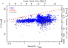 |
Fig. 1. Hubble K-band diagram for the initial sample (see Sect. 2.2). The stars signify QSOs, the circles galaxies and squares unclassified sources. The broken line shows the fit of de Breuck et al. (2002). |
2. Analysis and results
2.1. Photometry matching
For each source, we matched the coordinates to the closest source within a 6 arc-sec search radius in the NASA/IPAC Extragalactic Database (NED), from which we obtained the specific flux densities. We also used the NED names to query the Wide-Field Infrared Survey Explorer (WISE; Wright et al. 2010), the Two Micron All Sky Survey (2MASS; Skrutskie et al. 2006), and the Galaxy Evolution Explorer (GALEX data release GR6/7)2 databases. In order to ensure a uniform magnitude measure, if the frequency of the photometric point fell within Δlog10ν = ±0.05 of the central frequency of the band, the measurement was added (Fig. 2)3. For more than one point in the band the fluxes were averaged before the conversion to magnitude.
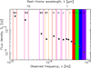 |
Fig. 2. Example of the photometric data points from a single source. The canonical band frequencies with Δlog10ν = ±0.05 are shown. |
Using the Large Area Radio Galaxy Evolution Spectroscopic Survey (LARGESS; Ching et al. 2017), Glowacki et al. (2019) find a correlation between redshift, the W1 (λ = 3.4 μm), and W2 (λ = 4.6 μm) magnitudes of WISE, which includes quasars (or at least, broad emission line sources). However, the spread is wide, with Glowacki et al. quoting regression coefficients of r = 0.56 and 0.36 for the W1 and W2-band fits, respectively. From our own matching, by source (NED) name, we obtain r = 0.77 and 0.65, respectively (Fig. 3).4 Although indicative of reasonable fits, when applied to our initial test sample, the “MgII sample” (Fig. 4), the regression coefficients drop, indicating that the W1 and W2 fits may not prove to be reliable photometric redshift predictors for other samples.
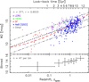 |
Fig. 3. Hubble W2-band diagram for the LARGESS sample. The dotted line shows the least-squares fit, with regression coefficient r, and the dot–dashed lines showing the ±1σ span of this. The filled squares signify high-excitation radio galaxies (HERGs), the unfilled stars low-excitation radio galaxies (LERGs), the circles star-forming (SF) galaxies and the filled stars broad emission line (AeB) sources (suspected quasars, Ching et al. 2017). The broken curve shows the fit of Glowacki et al. (2019) to the QSOs (their Table 2). The bottom panel shows the mean values in equally sized bins with the vertical error bars showing ±1σ and the horizontal bars the range. |
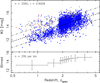 |
Fig. 4. As Fig. 3, but for our initial (the MgII) sample (see main text). Using W1 gives r = 0.4895 (n = 3400). As per Fig. 1, the stars signify QSOs, the circles galaxies and squares unclassified sources. |
2.2. MgII sample and initial testing
Our ultimate aim is to test the 3.3 million galaxies and QSOs in the Sloan Digital Sky Survey (SDSS) Data Release 12 (DR12, Alam et al. 2015), which we are currently querying for the full NED, WISE, 2MASS and GALEX photometries. This is expected to take several years to complete and so we initially tested the 23 659 sources illuminating MgII absorbers (Zhu & Ménard 2013) in the SDSS DR12. Of these, photometric data could be found for 17 285.
In order to find the best combination of magnitudes with which to obtain an estimator for the photometric redshift, we initially explored machine learning techniques. In the WEKA package (Hall et al. 2009), a suite of machine learning algorithms, only individual features (magnitudes) could be tested automatically with combinations having to be entered manually as features5. We therefore proceeded manually, performing exhaustive tests of various arithmetic combinations of magnitudes and colours. Although many of these may not have been meaningful (e.g. the multiplication of magnitudes), they were, nevertheless, tested as they may provide insight on how to proceed (Moss 2019).
Since small samples could yield large regression coefficients, in order to be flagged as a good fit, both |r| > 0.5 and r2n > 1000 were required. For the magnitude combinations, the best fit was given by U − I with r = 0.5887 and r2n = 2340. Of the colour combinations, there were several with |r| > 0.7 and r2n > 1000, with (I − W2)/(W3 − U) being one of the top five with r = 0.83 and r2n = 1360 (Fig. 5). The remaining four, which had slightly lower values of |r|, but slightly higher sample sizes, giving a higher r2n, had a complex physical interpretation, for example (B × W2)/(R × I), whereas (I − W2)/(W3 − U) is recognisable as a colour–colour relation.
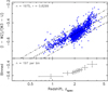 |
Fig. 5. Best fit model to the MgII sample. The dotted line shows the least-squares fit, giving (I − W2)/(W3 − U) = 0.448log10z − 0.655. |
2.3. SDSS DR12 – first 50 000 QSOs
While testing the initial sample, the data-mining of the SDSS DR12 was ongoing and we now discuss the first 50 000 QSOs with accurate spectroscopic redshifts (δz/z < 0.01). In Fig. 6, we show the photometric redshifts predicted for these from the MgII model. Although the fit is similar over the range covered by the MgII sample, this fails at z ≲ 1.
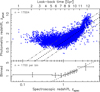 |
Fig. 6. Photometric redshifts predicted for the SDSS sample. The dotted line shows zpred = zspec, with the dot-dashed lines showing the ±1σ range. |
The W3, W2, I and U bands have central wavelengths of 12, 4.6, 0.806 and 0.365 μm, respectively, and so I − W2 and W3 − U trace the extreme red — NIR and NIR — ultraviolet colours, respectively. Looking at the colours individually (Fig. 7), both I − W2 and W3 − U decrease with redshift, although it is not clear why these should be particularly sensitive to the source redshift. However, it should be borne in mind that at z ≫ 0 these would have been emitted at significantly shorter wavelengths. For instance, at a redshift of z ∼ 1, the observed I − W2 and W3 − U colours are U − K and W2 − FUV in the rest-frame of the source, respectively (Fig. 8).
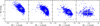 |
Fig. 7. (I − W2)/(W3 − U) colour–colour plot over various redshift ranges. The error bars show the ±1σ ranges around the mean. |
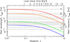 |
Fig. 8. Evolution of source-frame wavelength with redshift for W3, W2, I and U. These are overlaid upon the observed-frame NIR, optical and GALEX near-ultraviolet (NUV) and far-ultraviolet (FUV) bands. |
In order to fit the z ≲ 1 data, we tested further combinations of magnitudes, although, as expected from above, the combination (U − K)/(W2 − FUV) gives the best result (Fig. 9, left). In Fig. 6, we also note a departure from the zspec ≳ 1 trend at zspec ≳ 3, also evident as the increased scatter in the z > 3 panel of Fig. 7. At these redshifts, the rest-frame (U − K)/(W2 − FUV) combination will be approximately (J − W2.5)/(W4 − V) in the observed-frame, where we have dubbed the λ = 8.0 μm magnitude, located between the W2 (4.5 μm) and W3 (12 μm) bands, “W2.5”6. Possibly due to the limited data, it is in fact the observed (I − W2.5)/(W4 − B) which gives the tightest correlation with zspec, although the numbers remain small (Fig. 9, right).
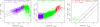 |
Fig. 9. As Fig. 6, fitting the observed-frame (U − K)/(W2 − FUV) for z < 1 (squares, left), (I − W2)/(W3 − U) for 1 ≤ z ≤ 3 (circles, middle) and (I − W2.5)/(W4 − R) for z > 3 (triangles, right). |
One issue with using a multi-component fit is deciding where the combination should be switched in the absence of a spectroscopic redshift. One possibility is to use the photometric redshift (e.g. Maddox et al. 2012), although, due to the flattening of the zphot—zspec relation at zphot ∼ 1, this is not helpful with zspec ≈ 0.1−2 being spanned for zphot ≈ 1 (Fig. 6). Various methods, which did not rely upon knowledge of the spectroscopic redshift, were trialled, but were unsuccessful. For example, using the value of (U − K)/(W2 − FUV), but, as seen from (Fig. 9, left), the variation of this combination with zspec exhibits a turnover at zspec ≈ 1, resulting in a degeneracy. The most straightforward and effective method was a switch at W2 ≈ 12.5 for (U − K)/(W2 − FUV) to (I − W2)/(W3 − U) and at W2 ≈ 15 for (I − W2)/(W3 − U) to (I − W2.5)/(W4 − B), based upon the loose W2–zspec relation (Fig. 4).
In Fig. 10, we show the resulting photometric redshifts obtained from the fits in Fig. 9. As seen from this, there is some scatter at zspec ≲ 0.5, due to the imperfect switch invoking the W2 magnitude, and at zspec ≳ 3, again, possibly due to an imperfect switch, in addition to the sparsely sampled data (Fig. 9, right). However, from z ≳ 0.5 up to the redshift limit of the data, the model is seen to give accurate statistical predictions of the photometric redshift.
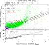 |
Fig. 10. Photometric redshifts predicted from the multi-component fit to the SDSS data (Fig. 9), shown on a linear scale to emphasise the high redshift range. The symbols are as per Fig. 9, in order to show the W2 switch of each point. |
3. Discussion
3.1. Application to radio-selected samples
Our model is constructed from an optically selected sample and here we test it upon several radio band datasets, which cover a wide range of redshifts. By using disparate and heterogeneous test samples, we hope to maximise the robustness of our model to other (future) datasets where information may be limited.
The LARGESS catalogue comprises 19 179 radio sources matched with SDSS counterparts, giving redshifts for 10 883 (Ching et al. 2017). Upon removing duplicate sight-lines, the U ∩ K ∩ W2 ∩ FUV, W3 ∩ W2 ∩ I ∩ U and I ∩ W2.5 ∩ W4 ∩ B requirements to cover all redshifts yielded only 250 sources, which is 2.3% of the sources with known redshifts. This compares to 85.6% for the W2 magnitude only (Glowacki et al. 2019), although our more stringent matching of sources will also contribute to the small numbers (see Sect. 2.2). From the fit (Fig. 11), we see that our model provides reasonable photometric redshifts for both AGN and non-AGN, deviating by a maximum of ≈1σ, at zspec ≈ 0.5, close to where the observed (U − K)/(W2 − FUV) to (I − W2)/(W3 − U) switch occurs.
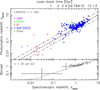 |
Fig. 11. Predicted redshifts for the LARGESS sample. |
The Second Realization of the International Celestial Reference Frame by Very Long Baseline Interferometry (ICRF2, Ma et al. 2009), constitutes a sample of strong flat spectrum radio sources, of which 1682 have known redshifts (Titov & Malkin 2009; Titov et al. 2013 and references therein). Of these 119 (8.0% of the sample)7 have all of the required magnitudes. Although the dataset is small (Fig. 12), accurate photometric redshifts are predicted for zspec ≳ 0.5, below which the data are sparser.
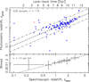 |
Fig. 12. As Fig. 11, but for the VLBI sample. As per Fig. 1, the stars signify QSOs, the circles galaxies and squares unclassified sources. |
In addition to the ICRF2, there are a multitude of radio source catalogues. However, these are generally lacking in spectroscopic information. Of those for which redshifts exist, the Combined ES-NVSS Survey Of Radio Sources (CENSORS) tested by Glowacki et al. (2019) has 143 redshifts (Brookes et al. 2008) and the GaLactic and Extragalactic All-sky Murchison Widefield Array (GLEAM) survey has 215 redshifts (Callingham et al. 2017)8. The Parkes Flat-Spectrum samples also have measured redshifts; the Parkes Half-Jansky Flat-Spectrum Sample (PHFS) with 277 (Drinkwater et al. 1997) and the Parkes Quarter-Jansky Flat-spectrum Sample (PQFS) with 470 (Jackson et al. 2002)9. Since these samples are relatively small, we use the redshifted radio sources searched in associated H I 21-cm absorption. This comprises 819 sources over redshifts of 0.002 ≤ z ≤ 5.19 (see Curran & Duchesne 2018; Curran et al. 2019, and references therein), in addition to providing a more heterogeneous (unbiased) sample than the aforementioned catalogues. Of these, the required magnitudes could be measured for 71 sources, giving a fraction of 8.7%. Again, the predicted photometric redshifts are statistically accurate down to redshifts of z ≲ 0.03, where galaxies dominate (Fig. 13).
3.2. Comparison with other studies
In Fig. 14, we show the distribution of Δz = zspec − zphot, which appears to be well fitted by a Gaussian, apart from the extended tail at Δz ≲ −0.7. We note also, that the different fits over the three W2 ranges (Fig. 9) give consistent results.
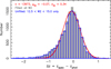 |
Fig. 14. Distribution of zspec − zphot over all redshifts with no source filtering. The unfilled histogram shows the 12.5 < W2 < 15.0 [observed-frame (I − W2)/(W3 − U)] data only and the filled all of the data [i.e. including the observed-frame (U − K)/(W2 − FUV) and (I − W2.5)/(W4 − R) data], to which the Gaussian is fitted. |
Other studies have also used (earlier releases of) SDSS data to yield narrower distributions of Δz, typically being σΔz ≈ 0.1, with 70% of the values being within |Δz| ≈ 0.2 (Richards et al. 2001; Weinstein et al. 2004; Ball et al. 2008; Maddox et al. 2012), whereas we require |Δz| = 0.4 to reach this fraction. These Gaussian fits are, however, considerably narrower than the distributions, which exhibit wide tails on both sides (see Appendix A). Furthermore, the methods employed by these studies are considerably more complex than the method presented here, invoking the evolution of the SDSS colours (e.g. Richards et al. 2001) or i − K (Maddox et al. 2012) with redshift (Fig. 15). This introduces a degeneracy, where a colour matches more than one spectroscopic redshift, requiring the use of specialised algorithms to break this. The test samples are also filtered, with the removal of redder sources (e.g. Richards et al. 2001) and the visual inspection of images being required before their inclusion (e.g. Maddox et al. 2012). Lastly, the tight zspec–zphot relationships are obtained over limited (photometric) redshifts 0.8 ≤ zphot ≤ 2.2 (Weinstein et al. 2004), 1.0 ≤ zphot < 3.5 (Maddox et al. 2012) and magnitudes (Ball et al. 2008).
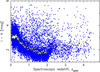 |
Fig. 15. I − K colour–redshift relation for our sample (cf. Fig. 13 of Maddox et al. 2012). The overlain error bars show the mean values in equally sized bins (of 100), spanning the error range (±1σ/10). |
Predicting the photometric redshifts of radio-selected data has been explored by Luken et al. (2018), who, through machine learning techniques, find ≈90% of the photometric redshifts to lie within a normalised residual of Δz/(zspec + 1)≤ ± 0.15. From our radio sample, which with 441 sources is of a similar size to the Luken et al. test samples (281–855), we find that only 60% of the sources have Δz/(zspec + 1)≤ ± 0.15 (Fig. 16), with 90% being reached at Δz/(zspec + 1)≲ ± 0.5. However, the Luken et al. data are concentrated at zspec ≲ 0.5, where the scatter being mitigated by the large zspec values in the denominator of the normalised residual, whereas the few data points at zspec ≳ 1 have Δz/(zspec + 1)≫ ± 0.15.
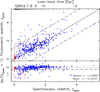 |
Fig. 16. All of the radio selected sources (Figs. 11–13) shown on a linear scale. The bottom panel shows the normalised residuals, with the dotted line showing the median value and the dashed line the mean. |
Lastly, we summarise Δz for our radio selected sources in Fig. 17. Although the numbers are small, the distribution is very similar that obtained from the optical data (Fig. 14), with an almost identical width and Δz ≲ −0.7 tail. We note also that, despite the apparent scatter introduced by the galaxies in the 21-cm sample (Fig. 13), these follow a similar distribution as the QSOs.
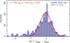 |
Fig. 17. Distribution of zspec − zphot over all redshifts with no source filtering for the radio-selected samples. The unfilled histogram shows the QSOs (quasars) only and the filled all of the data, to which the Gaussian is fitted. |
3.3. Magnitude limitations
Although the results are very promising, with the photometric redshifts of the radio selected sources being as accurate as from the optically selected parent sample, the requirement of four specific magnitude measurements per redshift regime significantly reduces the numbers (Table 1). From the table, we see the “bottleneck” in W3 ∩ W2 ∩ I ∩ U for the radio selected sources is due to the WISE magnitudes. From our testing, however, the λ = 4.6 μm and 12 μm far-infrared magnitudes are necessary for a reliable photometric redshift prediction (Sect. 2.2). Substituting the two WISE magnitudes for the Spitzer 5.8 μm (“W1.5”) and 8.0 μm (“W2.5”) values10, gives r = 0.4718 (n = 392) for (I − W1.5)/(W2.5 − U), cf. Fig 9 (middle). Substituting W1.5 for W1, thus restoring some of the W3 to W2 wavelength span improves upon this, with r = 0.5594 (n = 392), although the fit is still inferior to that of (I − W2)/(W3 − U).
3.4. Physical interpretation
It is remarkable that the (U − K)/(W2 − FUV) ratio provides a reliable tracer over such a wide redshift range, provided it is shifted accordingly to the corresponding observed-frame magnitudes (Fig. 9). The NIR emission in QSOs is believed to arise from hot dust in the circumnuclear material heated by the AGN (Hatziminaoglou et al. 2010), although de Breuck et al. (2002) suggest little contribution to the K-band NIR flux. This would suggest a stellar heated dust component and since the ultraviolet emission is responsible for the excess blue colour of the QSO (Shields 1978; Malkan & Sargent 1982), an increasing AGN contribution may be apparent as a decrease in U − K. From Fig. 18, we see that the AGN contribution, as traced by U − K does indeed increase with redshift, as expected from the Malmquist bias. However, for the W2 − FUV colour, which traces a wider range, inverted analogue of U − K, we see no correlation with redshift at zspec ≲ 1. At higher redshifts, however, where W2 approaches K in the rest-frame, a positive correlation is seen, which may be expected from the U − K anti-correlation.
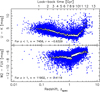 |
Fig. 18. Observed U − K and W2 − FUV colours versus redshift for the SDSS sample. The overlain error bars show the mean values in equally sized bins (of 100), spanning the error range (±1σ/10). In the bottom paneln = 4322 and r = −0.0366 for zspec < 1. |
This suggests that the U − K colour may be sufficient on its own to estimate the photometric redshift. This was attempted in order to increase the number of photometric redshifts for the radio sources (Sect. 3.3)11 and returned reasonable values (≤ ± 1σ of zspec) over 0.02 ≲ zspec ≲ 1. However, as seen in Fig. 18, there is a degeneracy between the observed U − K and zspec, which requires W2 in order to be broken. Hence, we suggest that the rest-frame U − K colour traces the excess pgflux due to the AGN and thus offers a measure of the redshift. While normalisation by W2 − FUV tightens the fit (increasing pg|r| = 0.63 to 0.73), the main contribution of this colour is to flag when the magnitudes should be switched in order to continue to trace the rest-frame U − K emission over a range of redshifts.
4. Conclusions
Given that an uncomplicated, source independent, method of obtaining reliable photometric redshifts will prove invaluable to the next generation of large extragalactic radio surveys, we have tested the feasibility of predicting these using near-infrared and visible pgmagnitudes. This builds upon the work of de Breuck et al. (2002), who find a tight correlation between the K-band magnitude and the redshift, although this only applies to galaxies. When applied to our initial test sample, which is dominated by bright point sources illuminating MgII absorption systems (mostly QSOs), we find that the fit of de Breuck et al. provides only a lower limit to the redshift, probably due to an additional contribution (from the AGN) to the near-infrared flux.
Recently, Glowacki et al. (2019) have estimated photometric redshifts from the WISE W1 and W2 bands in the LARGESS sample. However, with regression coefficients of r = 0.56 and 0.36, respectively, the spread is too wide to yield useful photometric redshift estimates, with poor predictions when applied to other datasets. We therefore test how various combinations of magnitudes are correlated with redshift in the 17 285 strong test (MgII) sample and find that the ratio of the I − W2 and W3 − U colours, gives a regression coefficient of r = 0.83 for the 1975 sources for which all four magnitudes were available. However, expansion of this to a 50 000 strong sample of QSOs in the SDSS DR12, shows that this fit fails at redshifts of z ≲ 1, where the MgII data are scarce. Further testing finds that the low redshift regime is best fitted by the ratio of U − K and W2 − FUV colours, which are essentially the I − W2 and W3 − U colours in the rest-frame. Likewise, at z ≳ 3 the correlation holds best for (I − W2.5)/(W4 − B), where W2.5 is the Spitzer 8.0 μm magnitude.
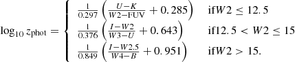
That is, the photometric redshift can be obtained from the rest-frame (U − K)/(W2 − FUV) colour ratio, over the 0.1 ≲ z ≲ 5 span of the data. However, given that we have no a priori knowledge of the redshift, we estimate this from the (weaker) W2 − z correlation, where we find W2 ≳ 12.5 at z ≳ 1 and W2 ≳ 15 at z ≳ 3. In terms of the observed-frame colours, the photometric redshift is thus obtained from
Self-testing this on the SDSS sample, the distribution is close to Gaussian with a mean Δz = −0.07 and a standard deviation of σΔz = 0.34. On first inspection this does not compete favourably with other studies, which find σΔz ≈ 0.1, although these have Δz wings significantly extended past the Gaussian and are only effective over limited redshift ranges, even after potential outliers have been removed. Furthermore, derivation of the photometric redshifts involve complex algorithms in order to break the degeneracies which arise via these methods.
Testing our model on the radio sources for which we have redshifts, the Δz distribution is very similar to that of the SDSS sample, which gives us confidence in the potential of this method to estimate the photometric redshifts of the vast majority of radio sources which lack the required spectroscopic information. The major drawback is that, although the requirement of four separate magnitude measurements is possible for 34% of the SDSS sources, this falls to 3–8% in the radio selected samples. This bottleneck is due to the limited number of WISE magnitudes, with the other magnitudes being available for over half of the sources (e.g. the I and U magnitudes for 12.5 < W2 ≤ 15, where the vast majority of sources are located).
Inspection of the colours shows that it is the rest-frame U − K colour which is anti-correlated with redshift, which would be expected if the ultraviolet emission traces the AGN activity with the far-infrared being dominated by stellar activity, thus providing an analogue of the K − z relation for galaxies. Reliance upon these two magnitudes only would vastly increase the applicability of this method as a photometric redshift predictor. However, the WISE bands are required to measure K at z ≳ 1 and W2 is required to estimate the redshift in order to apply the correct colour combination. Nevertheless, even a 2% rate will yield photometric redshifts for over one million of the sources expected to be detected with the Evolutionary Map of the Universe.
For instance, R ≲ 21 (Curran et al. 2013a) and B ≲ 23 (Curran et al. 2013b) give QH I ≳ 1056 s−1 at z ≳ 3.
This method was also used in Fig. 1.
This yielded far fewer (377, Fig. 3) sources with a W2 measure than the method of Glowacki et al. (2019), which matches 9294 of the LARGESS sources.
See Curran et al. (2016), Curran & Duchesne (2018) for examples.
The Spitzer Space Telescope (Capak et al. 2013) data are incorporated into the NED photometry search (Sect. 2.2).
Although very few could be matched to within 6 arc-sec of a NED source (see Sect. 2.1).
From 49 GHz peaked spectrum radio galaxies in the PHFS, de Vries et al. (2007) find a correlation between the R-band magnitude and the redshift. However, none of these sources has the full W3, W2, I, U combination.
The Spitzer 4.5 μm band is sufficiently close to W2 to be counted in the above analysis (Sect. 2.1), which also applies to the 3.6 μm band (λ = 3.4 μm for W1).
Ideally, the photometric redshifts for radio-selected samples would be obtained from the radio photometric pgproperties, although this is proving to be elusive (Majic 2015).
Acknowledgments
We wish to thank the referee for their helpful comments. This research has made use of the NASA/IPAC Extragalactic Database (NED) which is operated by the Jet Propulsion Laboratory, California Institute of Technology, under contract with the National Aeronautics and Space Administration. This research has also made use of NASA’s Astrophysics Data System Bibliographic Services.
References
- Alam, S., Albareti, F. D., Allende Prieto, C., et al. 2015, ApJS, 219, 12 [NASA ADS] [CrossRef] [Google Scholar]
- Allison, J. R., Sadler, E. M., Moss, V. A., et al. 2015, MNRAS, 453, 1249 [NASA ADS] [CrossRef] [Google Scholar]
- Allison, J. R., Sadler, E. M., Moss, V. A., et al. 2016, Astron. Nachr., 337, 175 [NASA ADS] [CrossRef] [Google Scholar]
- Allison, J. R., Moss, V. A., Macquart, J.-P., et al. 2017, MNRAS, 465, 4450 [Google Scholar]
- Ball, N. M., Brunner, R. J., Myers, A. D., et al. 2008, ApJ, 683, 12 [NASA ADS] [CrossRef] [Google Scholar]
- Brookes, M. H., Best, P. N., Peacock, J. A., Röttgering, H. J. A., & Dunlop, J. S. 2008, MNRAS, 385, 1297 [NASA ADS] [CrossRef] [Google Scholar]
- Callingham, J. R., Ekers, R. D., Gaensler, B. M., et al. 2017, ApJ, 836, 174 [NASA ADS] [CrossRef] [Google Scholar]
- Capak, P. L., Teplitz, H. I., Brooke, T. Y., Laher, R., & Science Center, S. 2013, Am. Astron. Soc. Meet. Abstr., 221, 340 [Google Scholar]
- Carilli, C. L., Menten, K. M., Reid, M. J., Rupen, M. P., & Yun, M. S. 1998, ApJ, 494, 175 [NASA ADS] [CrossRef] [Google Scholar]
- Ching, J. H. Y., Sadler, E. M., Croom, S. M., et al. 2017, MNRAS, 464, 1306 [NASA ADS] [CrossRef] [Google Scholar]
- Curran, S. J., & Duchesne, S. W. 2018, MNRAS, 476, 3580 [NASA ADS] [CrossRef] [Google Scholar]
- Curran, S. J., & Whiting, M. T. 2012, ApJ, 759, 117 [NASA ADS] [CrossRef] [Google Scholar]
- Curran, S. J., Whiting, M. T., Murphy, M. T., et al. 2006, MNRAS, 371, 431 [NASA ADS] [CrossRef] [Google Scholar]
- Curran, S. J., Whiting, M. T., Wiklind, T., et al. 2008, MNRAS, 391, 765 [NASA ADS] [CrossRef] [Google Scholar]
- Curran, S., Whiting, M. T., Sadler, E. M., & Bignell, C. 2013a, MNRAS, 428, 2053 [NASA ADS] [CrossRef] [Google Scholar]
- Curran, S. J., Whiting, M. T., Tanna, A., et al. 2013b, MNRAS, 429, 3402 [NASA ADS] [CrossRef] [Google Scholar]
- Curran, S. J., Duchesne, S. W., Divoli, A., & Allison, J. R. 2016, MNRAS, 462, 4197 [NASA ADS] [CrossRef] [Google Scholar]
- Curran, S. J., Hunstead, R. W., Johnston, H. M., et al. 2019, MNRAS, 484, 1182 [NASA ADS] [CrossRef] [Google Scholar]
- de Breuck, C., van Breugel, W., Stanford, S. A., et al. 2002, AJ, 123, 637 [NASA ADS] [CrossRef] [Google Scholar]
- de Vries, N., Snellen, I. A. G., Schilizzi, R. T., Lehnert, M. D., & Bremer, M. N. 2007, A&A, 464, 879 [NASA ADS] [CrossRef] [EDP Sciences] [Google Scholar]
- Drinkwater, M. J., Webster, R. L., Francis, P. J., et al. 1997, MNRAS, 284, 85 [NASA ADS] [Google Scholar]
- Glowacki, M., Allison, J. R., Sadler, E. M., Moss, V. A., & Jarrett, T. H. 2019, MNRAS, submitted [arXiv:1709.08634] [Google Scholar]
- Hall, M., Frank, E., Holmes, G., et al. 2009, SIGKDD Explor., 11, 10 [CrossRef] [Google Scholar]
- Han, B., Ding, H.-P., Zhang, Y.-X., & Zhao, Y.-H. 2016, Res. Astron. Astrophys., 16, 74 [NASA ADS] [Google Scholar]
- Hatziminaoglou, E., Omont, A., Stevens, J. A., et al. 2010, A&A, 518, L33 [NASA ADS] [CrossRef] [EDP Sciences] [Google Scholar]
- Jackson, C. A., Wall, J. V., Shaver, P. A., et al. 2002, A&A, 386, 97 [NASA ADS] [CrossRef] [EDP Sciences] [Google Scholar]
- Luken, K. J., Norris, R. P., & Park, L. A. F. 2018, PASP, submitted [arXiv:1810.10714] [Google Scholar]
- Ma, C., Arias, E. F., Bianco, G., et al. 2009, IERS Tech. Note, 35, 1 [NASA ADS] [Google Scholar]
- Maddox, N., Hewett, P. C., Péroux, C., Nestor, D. B., & Wisotzki, L. 2012, MNRAS, 424, 2876 [NASA ADS] [CrossRef] [Google Scholar]
- Majic, R. A. M. 2015, Radio Photometric Redshifts: Estimating Radio Source Redshifts from Their Spectral Energy Distributions, Tech. rep. (Victoria University of Wellington) [Google Scholar]
- Malkan, M. A., & Sargent, W. L. W. 1982, ApJ, 254, 22 [NASA ADS] [CrossRef] [Google Scholar]
- Morganti, R., Sadler, E. M., & Curran, S. 2015, Advancing Astrophysics with the Square Kilometre Array (AASKA14), 134 [CrossRef] [Google Scholar]
- Moss, J. P. 2019, Master’s Thesis, Victoria University of Wellington, New Zealand [Google Scholar]
- Norris, R. P., Hopkins, A. M., Afonso, J., et al. 2011, PASA, 28, 215 [NASA ADS] [CrossRef] [Google Scholar]
- Norris, R. P., Salvato, M., Longo, G., et al. 2019, PASP, submitted [arXiv:1902.05188] [Google Scholar]
- Polsterer, K. L., Zinn, P.-C., & Gieseke, F. 2013, MNRAS, 428, 226 [NASA ADS] [CrossRef] [Google Scholar]
- Richards, G. T., Weinstein, M. A., Schneider, D. P., et al. 2001, AJ, 122, 1151 [NASA ADS] [CrossRef] [Google Scholar]
- Salvato, M., Ilbert, O., & Hoyle, B. 2019, Nat. Astron., 3, 212 [NASA ADS] [CrossRef] [Google Scholar]
- Shields, G. A. 1978, Nature, 272, 706 [NASA ADS] [CrossRef] [Google Scholar]
- Skrutskie, M. F., Cutri, R. M., Stiening, R., et al. 2006, AJ, 131, 1163 [NASA ADS] [CrossRef] [Google Scholar]
- Titov, O., & Malkin, Z. 2009, A&A, 506, 1477 [NASA ADS] [CrossRef] [EDP Sciences] [Google Scholar]
- Titov, O., Stanford, L. M., Johnston, H. M., et al. 2013, AJ, 146, 10 [NASA ADS] [CrossRef] [Google Scholar]
- Webster, R. L., Francis, P. J., Peterson, B. A., Drinkwater, M. J., & Masci, F. J. 1995, Nature, 375, 469 [NASA ADS] [CrossRef] [Google Scholar]
- Weinstein, M. A., Richards, G. T., Schneider, D. P., et al. 2004, ApJS, 155, 243 [NASA ADS] [CrossRef] [Google Scholar]
- Willott, C. J., Rawlings, S., Jarvis, M. J., & Blundell, K. M. 2003, MNRAS, 339, 173 [NASA ADS] [CrossRef] [Google Scholar]
- Wright, E. L., Eisenhardt, P. R. M., Mainzer, A. K., et al. 2010, AJ, 140, 1868 [NASA ADS] [CrossRef] [Google Scholar]
- Zhu, G., & Ménard, B. 2013, ApJ, 770, 130 [NASA ADS] [CrossRef] [Google Scholar]
Appendix A: Comparison with machine learning methods: k-nearest neighbour
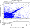 |
Fig. A.1. Photometric redshifts of the SDSS sample obtained from the k-nearest neighbour algorithm, with no source filtering. The standard deviation of σ = 0.8840 gives a standard error of |


As stated in Sect. 3.2, machine learning techniques are often used to obtain the photometric redshift. One such method is the k-nearest neighbour (kNN) algorithm, which compares the Euclidean distance between a test sample point and its k nearest neighbours in a feature space, comprising such properties as magnitude, colour or luminosity. It then assigns a weighted combination of the redshifts of those nearest neighbours to the test object in order to place it into a group. This method has been tested extensively on SDSS data, with the u − g, g − r, r − i and i − z colours giving the best results (e.g. Ball et al. 2008; Polsterer et al. 2013; Han et al. 2016). For our sample of 50 000 QSOs from the SDSS DR12, this complete set of colours could be found for 48 490. Using half the sample to train the model, we obtain the photometric redshifts shown in Fig. A.1. The distribution has a similar shape to that of Han et al. (2016), who apply support vector machine methods on top of the kNN algorithm. From the binned data, we see that the large apparent spread at low redshift is countered by a large population of sources for which zphot ≈ zspec, giving reasonable statistical accuracy at zspec ≲ 2, although the mean photometric redshift is underestimated at higher redshifts.
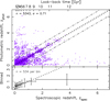 |
Fig. A.3. Photometric redshifts of the radio source sample obtained from the k-nearest neighbour algorithm, with no source filtering. |
In Fig A.2, we show the corresponding distribution of Δz = zspec − zphot. Although the Gaussian fit is narrow, like the other studies utilising the SDSS colours (e.g. Richards et al. 2001; Weinstein et al. 2004; Ball et al. 2008; Maddox et al. 2012), we find the same wide tails, resulting in a non-Gaussian (fat/heavy-tailed) distribution. Specifically, the Gaussian fit gives μΔz = 0.001 and σΔz = 0.119, although the data themselves have μΔz = −0.011 and σΔz = 0.885. This compares to a fit of μΔz = −0.070 and σΔz = 0.345 using our method, with the data giving μΔz = −0.174 and σΔz = 0.557 (Fig. 14).
We also apply the kNN algorithm to the radio selected sources (Sect. 3.1), where the requirement of only five (optical) magnitudes, vastly increases the sample (10 707 cf. our 410). Again, using half of the data to train the algorithm, we obtain a very similar distribution as the SDSS sample (Fig. A.3), where, again, this underestimates the redshift at zspec ≳ 2. Showing the Δz distribution (Fig. A.4), broad wings are again apparent, with the Gaussian fit underestimating the spread of the data, which have μΔz = 0.009 and σΔz = 0.705. This compares to μΔz = −0.255 and σΔz = 0.787 using our method (Fig. 17), which, again, appears to be more accurate at high redshift (Figs. 11–13).
The machine learning techniques offer a comparable accuracy to our method, with the narrow Δz ≈ 0 peak being countered by broad wings, whereas we obtain a generally wider spread but a more Gaussian distribution. Although the large number of magnitudes required for our method vastly reduces the sample size, we do not require a training set and the colour ratios we employ have a clearer physical interpretation, giving insight into the AGN contribution to the colour (Sect. 3.4). It is thus apparent that our method provides a useful independent means with which to determine the photometric redshift, thus providing another string in the bow in determining this for the large sample of objects expected from forthcoming large radio surveys.
All Tables
All Figures
|
Fig. 1. Hubble K-band diagram for the initial sample (see Sect. 2.2). The stars signify QSOs, the circles galaxies and squares unclassified sources. The broken line shows the fit of de Breuck et al. (2002). |
| In the text | |
|
Fig. 2. Example of the photometric data points from a single source. The canonical band frequencies with Δlog10ν = ±0.05 are shown. |
| In the text | |
|
Fig. 3. Hubble W2-band diagram for the LARGESS sample. The dotted line shows the least-squares fit, with regression coefficient r, and the dot–dashed lines showing the ±1σ span of this. The filled squares signify high-excitation radio galaxies (HERGs), the unfilled stars low-excitation radio galaxies (LERGs), the circles star-forming (SF) galaxies and the filled stars broad emission line (AeB) sources (suspected quasars, Ching et al. 2017). The broken curve shows the fit of Glowacki et al. (2019) to the QSOs (their Table 2). The bottom panel shows the mean values in equally sized bins with the vertical error bars showing ±1σ and the horizontal bars the range. |
| In the text | |
|
Fig. 4. As Fig. 3, but for our initial (the MgII) sample (see main text). Using W1 gives r = 0.4895 (n = 3400). As per Fig. 1, the stars signify QSOs, the circles galaxies and squares unclassified sources. |
| In the text | |
|
Fig. 5. Best fit model to the MgII sample. The dotted line shows the least-squares fit, giving (I − W2)/(W3 − U) = 0.448log10z − 0.655. |
| In the text | |
|
Fig. 6. Photometric redshifts predicted for the SDSS sample. The dotted line shows zpred = zspec, with the dot-dashed lines showing the ±1σ range. |
| In the text | |
|
Fig. 7. (I − W2)/(W3 − U) colour–colour plot over various redshift ranges. The error bars show the ±1σ ranges around the mean. |
| In the text | |
|
Fig. 8. Evolution of source-frame wavelength with redshift for W3, W2, I and U. These are overlaid upon the observed-frame NIR, optical and GALEX near-ultraviolet (NUV) and far-ultraviolet (FUV) bands. |
| In the text | |
|
Fig. 9. As Fig. 6, fitting the observed-frame (U − K)/(W2 − FUV) for z < 1 (squares, left), (I − W2)/(W3 − U) for 1 ≤ z ≤ 3 (circles, middle) and (I − W2.5)/(W4 − R) for z > 3 (triangles, right). |
| In the text | |
|
Fig. 10. Photometric redshifts predicted from the multi-component fit to the SDSS data (Fig. 9), shown on a linear scale to emphasise the high redshift range. The symbols are as per Fig. 9, in order to show the W2 switch of each point. |
| In the text | |
|
Fig. 11. Predicted redshifts for the LARGESS sample. |
| In the text | |
|
Fig. 12. As Fig. 11, but for the VLBI sample. As per Fig. 1, the stars signify QSOs, the circles galaxies and squares unclassified sources. |
| In the text | |
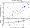 |
Fig. 13. As Fig. 12, but for the radio sources searched in H I 21-cm absorption. |
| In the text | |
|
Fig. 14. Distribution of zspec − zphot over all redshifts with no source filtering. The unfilled histogram shows the 12.5 < W2 < 15.0 [observed-frame (I − W2)/(W3 − U)] data only and the filled all of the data [i.e. including the observed-frame (U − K)/(W2 − FUV) and (I − W2.5)/(W4 − R) data], to which the Gaussian is fitted. |
| In the text | |
|
Fig. 15. I − K colour–redshift relation for our sample (cf. Fig. 13 of Maddox et al. 2012). The overlain error bars show the mean values in equally sized bins (of 100), spanning the error range (±1σ/10). |
| In the text | |
|
Fig. 16. All of the radio selected sources (Figs. 11–13) shown on a linear scale. The bottom panel shows the normalised residuals, with the dotted line showing the median value and the dashed line the mean. |
| In the text | |
|
Fig. 17. Distribution of zspec − zphot over all redshifts with no source filtering for the radio-selected samples. The unfilled histogram shows the QSOs (quasars) only and the filled all of the data, to which the Gaussian is fitted. |
| In the text | |
|
Fig. 18. Observed U − K and W2 − FUV colours versus redshift for the SDSS sample. The overlain error bars show the mean values in equally sized bins (of 100), spanning the error range (±1σ/10). In the bottom paneln = 4322 and r = −0.0366 for zspec < 1. |
| In the text | |
|
Fig. A.1. Photometric redshifts of the SDSS sample obtained from the k-nearest neighbour algorithm, with no source filtering. The standard deviation of σ = 0.8840 gives a standard error of |
| In the text | |
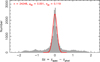 |
Fig. A.2. zspec − zphot distribution of the SDSS sample from the kNN algorithm (Fig. A.1). |
| In the text | |
|
Fig. A.3. Photometric redshifts of the radio source sample obtained from the k-nearest neighbour algorithm, with no source filtering. |
| In the text | |
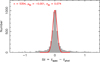 |
Fig. A.4. zspec − zphot distribution of the radio source sample from the kNN algorithm (Fig. A.3). |
| In the text | |
Current usage metrics show cumulative count of Article Views (full-text article views including HTML views, PDF and ePub downloads, according to the available data) and Abstracts Views on Vision4Press platform.
Data correspond to usage on the plateform after 2015. The current usage metrics is available 48-96 hours after online publication and is updated daily on week days.
Initial download of the metrics may take a while.