| Issue |
A&A
Volume 629, September 2019
|
|
|---|---|---|
| Article Number | A53 | |
| Number of page(s) | 17 | |
| Section | Galactic structure, stellar clusters and populations | |
| DOI | https://doi.org/10.1051/0004-6361/201935995 | |
| Published online | 04 September 2019 | |
Horizontal branch morphology: A new photometric parametrization
1
Department of Physics, Università di Roma Tor Vergata, Via della Ricerca Scientifica 1, 00133 Roma, Italy
2
INAF-Osservatorio Astronomico di Roma, Via Frascati 33, 00078 Monte Porzio Catone, Italy
e-mail: This email address is being protected from spambots. You need JavaScript enabled to view it.
3
NRC-Herzberg, Dominion Astrophysical Observatory, 5071 West Saanich Road, Victoria, BC V9E 2E7, Canada
4
Astrophysics Research Institute, Liverpool John Moores University, IC2 Building, Liverpool Science Park, 146 Brownlow Hill, Liverpool L3 5RF, UK
5
INAF-Osservatorio Astronomico di Capodimonte, Salita Moiariello 16, 80131 Napoli, Italy
6
IAC – Instituto de Astrofisica de Canarias, Calle Via Lactea s/n, 38205 La Laguna, Spain
7
Departamento de Astrofisica, Universidad de La Laguna, Avenida Astrofísico Francisco Sánchez s/n, 38200 Tenerife, Spain
8
INAF – Osservatorio Astronomico d’Abruzzo, Via Mentore Maggini snc, Loc. Collurania, 64100 Teramo, Italy
Received:
31
May
2019
Accepted:
19
July
2019
Abstract
Context. Theory and observations indicate that the distribution of stars along the horizontal branch of Galactic globular clusters mainly depends on the metal content. However, the existence of globular clusters with similar metal content and absolute age but different horizontal branch morphologies, suggests the presence of another parameter affecting the star distribution along the branch.
Aims. To investigate the variation of the horizontal branch morphology in Galactic globular clusters, we define a new photometric horizontal branch morphology index, overcoming some of the limitations and degeneracies affecting similar indices available in the literature.
Methods. We took advantage of a sample of 64 Galactic globular clusters, with both space-based imaging data (Advanced Camera for Surveys survey of Galactic globular clusters) and homogeneous ground-based photometric catalogues in five different bands (U, B, V, R, I). The new index, τHB, is defined as the ratio between the areas subtended by the cumulative number distribution in magnitude (I) and in colour (V − I) of all stars along the horizontal branch.
Results. This new index shows a linear trend over the entire range in metallicity (−2.35 ≤ [Fe/H] ≤ −0.12) covered by our Galactic globular cluster sample. We found a linear relation between τHB and absolute cluster ages. We also found a quadratic anti-correlation with [Fe/H], becoming linear when we eliminate the age effect on τHB values. Moreover, we identified a subsample of eight clusters that are peculiar according to their τHB values. These clusters have bluer horizontal branch morphology when compared to typical ones of similar metallicity. These findings allow us to define them as the ’second parameter’ clusters in the sample. A comparison with synthetic horizontal branch models suggests that they cannot be entirely explained with a spread in helium content.
Key words: stars: horizontal-branch / globular clusters: general
© ESO 2019
1. Introduction
Globular clusters are stellar systems that play a fundamental role in constraining the formation and evolution of galaxies (Searle & Zinn 1978; VandenBerg et al. 2013; Leaman et al. 2013) and cosmological parameters. Dating back more than half a century (Sandage 1953), the absolute ages of Galactic globular clusters (GGCs) have been used to provide a lower limit to the age of the Universe (see e.g. Salaris & Weiss 2002; Dotter et al. 2011; Monelli et al. 2015; Richer et al. 2013, and references therein) and estimate of the primordial helium abundance (see e.g. Zoccali et al. 2000; Salaris & Cassisi 2005; Villanova et al. 2012). GGCs are also laboratories to investigate evolutionary (Chaboyer et al. 2017; Dotter et al. 2007; Brown et al. 2010; Weiss et al. 2004) and pulsational (Bono & Stellingwerf 1994; Bono et al. 1999; Marconi et al. 2015) properties of old, low-mass stars. In this context, advanced evolutionary phases (red giant [RGs] and horizontal branch [HB] stars) have several advantages when compared with main sequence (MS) stars. They are a few magnitudes brighter and within the reach of spectroscopic investigations at the 8−10 m class telescopes. This means that they can be used for investigating the cluster dynamical evolution and interaction with the Galactic potential (Pancino et al. 2007; Zocchi et al. 2017; Calamida et al. 2017; Lanzoni et al. 2018). Moreover, their chemical abundances (iron peak, α-, neutron capture elements) can be measured with high accuracy both in the optical (Carretta et al. 2014) and in the near-infrared (NIR) regime (D’Orazi et al. 2018).
Despite a general consistency between theory and observations concerning hydrogen and helium burning phases, we continue to face a number of long-standing open questions. Amongst them the morphology of the HB plays a pivotal role. Stars along the HB are low-mass (M ≈ 0.50−0.80 M⊙), core-helium-burning stars and their distribution along the HB depends, at fixed initial chemical composition, on their envelope mass. Indeed, the envelope mass when moving from the red HB (RHB) to the extreme HB (EHB) decreases from Menv ≈ 0.30 M⊙ to Menv ≈ 0.0001 M⊙, while the effective temperature increases from ≈5500 K to ≈30 000 K.
The current empirical and theoretical evidence indicates that the HB morphology is affected by the initial metal content. Metal-poor clusters are mainly characterized by a blue HB morphology. This means that in these clusters HB stars are mainly distributed along the blue, hot, and extremely hot region. Metal-rich GGCs are generally characterized by a red HB morphology, that is, HB stars in these clusters are mainly distributed in the red (cool) region.
Although this theoretical and empirical framework appears well established, there is solid evidence that GGCs with similar chemical compositions display different HB morphologies. This suggests that the HB morphology was affected by at least a “second parameter” (see e.g. Sandage & Wildey 1967, and references therein). This problem was defined as the “second parameter problem” and the clusters affected by this problem were called second parameter clusters.
During the last half-century several working hypotheses have been suggested to explain the second parameter problem. They include variations of the initial helium content (van den Bergh 1967; Sandage & Wildey 1967), dynamical effects related to the cluster mass (e.g. Recio-Blanco et al. 2006), the cluster age (e.g. Searle & Zinn 1978), dynamical evolution (e.g. Iannicola et al. 2009), or a combination of two or more of these – for example age and/or metallicity plus helium content, as suggested by Freeman & Norris (1981), Gratton et al. (2010).
To quantify the extent of this second parameter problem, Lee (1989), Lee et al. (1994) suggested an HB morphology index based on star counts along the HB. It is defined as the difference between the number of stars that are bluer (B) and redder (R) than the RR Lyrae (RRL) instability strip, divided by the sum of the number of blue, red, and variable (V) stars:  . This HB morphology index has been quite popular, because it can be easily estimated from the theoretical and the observational point of view (star counts). However, it is prone to intrinsic degeneracies in both the metal-poor and the metal-rich regimes, in the sense that when the observed HB is bluer or redder than the RRL strip, HBR stays constant, irrespectively of the exact distribution of stars along the HB.
Similar HB morphology indices have been suggested in the literature, but using different cuts in colour. In particular, Buonanno (1993) suggested splitting HB stars bluer than the RRL instability strip into two blocks: stars hotter than the RRL instability strip and cooler than (B − V) = −0.02 were called B1, while those hotter than (B − V) = −0.02 were called B2. The new index had the key advantage of removing the degeneracy of the HBR index in the metal-poor regime, but it was still affected by degeneracies in the metal-rich regime.
Considering that almost all GGCs show the presence of multiple populations, Milone et al. (2014) introduced two new indices for describing the HB morphology. L1 is the difference in colour between the red giant branch (RGB) and the coolest red point of the HB, while L2 is the colour extension of the HB. These two indices allowed the authors to identify three different GGC groups from the L1-[Fe/H] diagram, and to find correlations of L1 with cluster age and metallicity. In addition, they found a variation of L2 with cluster luminosity (mass) and with helium content. This latter correlation is connected with the presence of multiple populations in globular clusters and it could be an additional ingredient to explain the HB colour extension. These two parameters are interesting, because they are correlated with the physics characterizing the HB stars. However, their definition seems to be very sensitive to the choice of the key points selected in colour magnitude diagrams (HB luminosity level, RGB).
In this work, we introduce a new HB morphology index based on the ratio between the areas subtended by the cumulative number distribution (CND) of star counts along the observed cluster HB in magnitude (I-band) and in colour (V − I): τHB = ACND(I)/ACND(V − I). This new index has been calculated in a large sample (64) of GGCs, for which both space- and ground-based optical photometric catalogues are available. For the same sample of GGCs, we have also estimated the classical HBR index and performed a detailed comparison with τHB. We present evidence that our new index, in contrast with similar indices available in the literature, shows a well-defined correlation with cluster age and an anti-correlation with cluster iron abundance.
The structure of the paper is the following. We present in Sect. 2 our sample of GGCs with their photometric coverage. We also describe the method adopted for the separation between candidate cluster and field stars based on the comparison of star spectral energy distributions (SEDs). Section 3 deals with the classical HB morphology index HBR. We analyse its pros and cons and calculate its values for the entire cluster sample, together with its dependence on age and metallicity, while in Sect. 4 we do the same analysis for the L1 and L2 indices. In Sect. 5 we introduce our new HB morphology index, τHB, calculate its values for our GGC sample, and discuss pros and cons compared to HBR. In Sect. 6 we analyse and compare the relative difference between the classical HB morphology index and τHB estimates when considering just space- or just ground-based observations. The correlation of our new index with the absolute age and the metallicity of the individual clusters is addressed in Sect. 7. Here we also identify the second parameter clusters in our sample that show very different estimates in τHB compared to the ones attained by globulars with similar [Fe/H] values. In Sect. 8 we compare τHB with synthetic HB models specifically computed for this work. The summary of the results and a brief discussion concerning future developments of the project are outlined in Sect. 9. In Appendix A we list specific information on individual GGCs for which the photometric properties are uncertain either due to the lack of ground-based or space-based data, because the photometry does not cover the entire cluster area (tidal radius), or because of the small number of HB stars. In Appendix B we also included a few notes for the GGCs we defined as “outliers” in the analysis of the HB morphology.
2. Globular cluster sample
In this work we use a sample of 64 GGCs for which optical images are available from both space-based (Advanced Camera for Surveys (ACS)/Wide Field Channel (WFC) on board the Hubble Space Telescope (HST)) and ground-based observations. The relevant parameters for our cluster sample are listed in Table 1.
Globular Clusters in the sample with parameters used in this work.
We took advantage of the photometric catalogues provided by Sarajedini et al. (2007), Dotter et al. (2011) in the context of the Hubble Space Telescope Treasury project, An ACS Survey of Galactic Globular Clusters1. This survey is based on a single ACS pointing across the centre of each cluster, observed through two complete orbits, one for the F606W (∼V) and one for the F814W (∼I). Cluster NGC 6715 represents an exception since it was observed for two orbits in each filter (Anderson et al. 2008). Thanks to these data we can avoid the crowding problems in the central regions of the clusters (the red region in Fig. 1 shows the field coverage for one of the globulars in the sample, NGC 5053) and reach very faint magnitudes (I ∼ 26.0, see ACS colour-magnitude diagram (CMD) in Fig. 2).
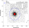 |
Fig. 1. Sky distribution of ground-based (black dots) and space-based (red dots) data for the cluster NGC 5053. North is up and east is to the left. |
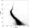 |
Fig. 2. Cluster NGC 5286 I, V − I CMD based only on ACS-HST data. |
To cover a significant fraction of the body of each cluster we adopted the multi-band (U, B, V, R, I) optical catalogues provided by one of the authors (PBS, see for example Stetson et al. 2005, 2014, 2019), based on images collected with several ground-based telescopes. The ground-based data allow us to reach the tidal radius for most of the globulars. The blue line in Fig. 1 shows the tidal radius of NGC 5053. There are a few clusters (see Appendix A) for which we cannot reach the tidal radius with our data while still covering the main body of the cluster. For 47 GGCs we have data in all available photometric bands from both space- and ground-based facilities.
Thanks to the fact that all the clusters in the sample have data in B, V, I bands (except for NGC 6426, NGC 6624, NGC 6652, Lynga 7, and Palomar 2, see Appendix A), we based the cluster and field stars’ separation on the SED of the stars in these bands, following the procedure described in Di Cecco et al. (2015), Calamida et al. (2017). We selected first the bona fide cluster stars considering only the central region, since we expect that it is less contaminated by field stars. Then we compared the SEDs of these stars to the ones in the total catalogue, to separate cluster stars from the field. We note that for stars with space data only we did not make any selection, because we expect negligible contamination by field stars in the ACS field of view (FoV). Therefore, in this case we took advantage of the entire ACS catalogues.
Moreover, when we had measurements in the V and I bands from both ACS and ground-based telescopes, we preferred the first ones for their higher signal-to-noise ratio (S/N) values. We used the ACS coverage for the central region of our globulars within the ACS FoV (∼4′), while outside up to the tidal radius we adopted the ground-based observations.
An example of our selection is shown in Fig. 3, which displays the V, B − I CMD of NGC 5286 for total (left panel), cluster (central panel), and field (right panel) stars. We can appreciate from the figure that the joint catalogues allow us to cover the entire evolution of the stars in the globulars, from the faint part of the MS to the brighter region of the RGB-tip and asymptotic giant branch (AGB) in the CMD.
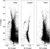 |
Fig. 3. Cluster NGC 5286 V, B − I CMD. Left panel: all stars. Central panel: our candidate cluster stars. Right panel: candidate field stars. Candidate cluster and field stars have been selected following the method described in the main text. |
3. The HBR morphology index
As already discussed in Sect. 1, the traditional HB morphology index is defined as
 (1)
(1)
where B is the number of HB stars bluer than the blue (hot) edge of the RRL instability strip, V is the number of RR Lyrae stars, and R is the number of HB stars redder than the red (cold) edge of the RRL instability strip. This HB morphology index has several advantages when compared with other observables (HB luminosity level, colour distribution) connected with the helium burning phases.
First, when considered with the comparison between predicted and observed HB luminosity levels, HB star counts are independent of uncertainties affecting the cluster distance and are minimally affected by uncertainties in cluster reddening and the possible occurrence of differential reddening. Moreover, the comparison between the predicted and observed number of HB stars is less prone to uncertainties affecting the transformations of theoretical predictions into the observational plane.
In the comparison between theory and observations, the HBR index accounts for the global distribution of stars along the HB. On the other hand, the comparison between the predicted and observed HB luminosity levels is mainly restricted to the RRL instability strip, that is, the truly horizontal region of the HB. However, a minor fraction of GGCs hosts a sizeable sample of RRLs to properly define the HB luminosity level.
One of the main cons of the HBR index is that it describes a global property of HB stars. This means that it does not trace the detailed stellar distribution along the HB. It is also affected by severe degeneracies both in the metal-poor and in the metal-rich regimes. This means that a significant fraction of GGCs attain values close either to 1 (blue HB morphology) or to −1 (red HB morphology), irrespective of the exact colour distribution of stars.
Despite the stated limitations we calculated values of the HBR index for our GGC sample. For each cluster we defined two boxes including candidate blue (B) and red (R) HB stars. The colour ranges for the boxes were fixed using either predicted or empirical edges for the RRL instability strip. Stars located in the RRL instability strip were neglected. To account for the number of variables we took advantage of the Clement catalogue of variable stars in GGCs. This catalogue was originally presented in Clement et al. (2001), but it is constantly updated2. For each cluster, it gives the number of variable stars together with their main pulsation parameters: pulsation period, mean magnitude and colour, and luminosity amplitude. For our analysis we took into account only confirmed cluster RRL stars, meaning that candidate cluster RRLs were not included.
Throughout our analysis, we adopted the homogeneous metallicity scale provided by Carretta et al. (2009). The authors estimated the iron abundances from high resolution spectra collected with the Fibre Large Srray Multi Element Spectrograph (FLAMES) at the Very Large Telescope (VLT), covering the entire metallicity range of GGCs. To increase the sample size they also re-calibrated the most common metallicity scales available in the literature (Zinn & West 1984; Kraft & Ivans 2003; Carretta & Gratton 1997). For two clusters in our sample (NGC 6624 and Lynga 7) we adopted the metallicity estimate available in the 2010 version of the Harris (1996) catalogue3.
To validate the current estimates of the HBR index with similar estimates available in the literature, Fig. 4 shows the comparison of our values with those provided by Harris in the 2003 version of his catalogue (Harris 1996). Data plotted in this figure show that both sets agree well over the entire metallicity range. Indeed, the difference is on average smaller than 20%. There are a few outliers (NGC 1851 and NGC 4590) for which the difference is approximately 30%−40%, but they are affected by a higher field-star contamination than the others, despite our homogeneous cluster and field star separation.
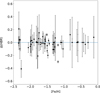 |
Fig. 4. Difference between Harris (1996) values (2003 version) for HBR and our measurements as a function of [Fe/H]. |
For each GGC in our sample, Table 2 gives its name (Cols. 1 and 2), the metallicity (Col. 3), and the number of blue (B) and red (R) stars (Cols. 4 and 5). In Col. 6 the values of the HBR’ index, defined as HBR′ = HBR + 2, are listed. The reason for this change is the following. From Fig. 4 we can see that the errors on the HBR index are small and not realistic. We define the uncertainty of the measured HBR as
 (2)
(2)
Parameters and observational HB morphology indices for the GGCs in the sample.
which takes into account the Poisson uncertainties in the star counts. The errors provided by this formula vanish as soon as B and R attain similar values, that is when HBR approaches zero. This is an intrinsic limitation affecting the definition of the HBR index. To overcome this problem we decided to use HBR′.
To investigate the dependence of the HB morphology on intrinsic cluster parameters, Fig. 5 shows the HBR′ index as a function of iron content for the current sample. Data plotted in this figure display some well established correlations. The HB morphology becomes systematically bluer when moving from metal-poor to more metal-rich GGCs.
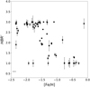 |
Fig. 5. Observed HBR′ values as a function of metal content. The metallicity scale is from Carretta et al. (2009) (see the appendix for more details). The error bar in the lower left corner gives the uncertainty of the metal content (0.1 dex). |
There is a well-defined degeneracy in the metal-intermediate regime (−1.6 ≤ [Fe/H] ≤ −1) in which GGCs with very similar metal abundances (the typical error on cluster metallicity being on the order of 0.1 dex – see horizontal error bar in the left bottom corner) cover a broad range in HBR′ values. This means a variation from a very blue to a very red HB morphology, the well known second parameter problem. Figure 5 shows that HBR′ is affected by degeneracy in its extreme values, HBR′ ∼ −1 (metal-rich regime) and HBR′ ∼ + 1 (metal-poor regime). This means that HBR′ has a low dynamical range attaining similar values for clusters with different metallicity.
Cluster age has been considered together with iron content as one of the main culprits affecting the HB morphology. We took advantage of the homogeneous cluster age estimates provided by VandenBerg et al. (2013), Leaman et al. (2013) for the same GGCs, to investigate the correlation with HBR′ index. They estimated the cluster ages as follows. Firstly, they de-reddened the HB stars and then estimated the absolute visual magnitude by fitting a theoretical zero-age horizontal branch (ZAHB) to the lower bound of the HB star distributions. The absolute age of the globulars is estimated by the isochrone which, at fixed chemical composition, best matches the CMD from the main sequence turn off (MSTO) point to the beginning of the sub giant branch (SGB). Data plotted in Fig. 6 show that the HB morphology, at fixed cluster age, can move from very blue to very red. Indeed, the HBR′ index, within the uncertainty on the cluster age (∼1 Gyr, displayed by the error bar in the left bottom corner), ranges from 1 to 3. This evidence shows that the HBR′ index does not show any relevant correlation either with cluster age or with iron content.
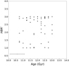 |
Fig. 6. Observed HBR′ values as a function of the cluster ages (gigayears (Gyr)) provided by VandenBerg et al. (2013), Leaman et al. (2013). The error bar in the lower left corner gives the uncertainty in the cluster ages (±0.5 Gyr). |
In the figure a significant fraction of GGCs is located around the two extreme values attained by the HBR′ index, namely 1 (eight globulars) and 3 (ten globulars). This means that the weak sensitivity of the HBR′ index does not allow us to properly trace the variation of the HB morphology when moving from metal-poor to metal-rich globulars, while the HBR′ index manages to trace the variation of the HB morphology in the metal-intermediate regime, where the relation appears to be almost linear. From the HBR′-age plane we can merely identify three different groups of clusters, with of HBR′ ∼+1, ∼+2, and ∼+3, respectively.
4. L1 and L2 HB morphology indices
A new approach to parametrize the HB properties has been recently proposed by Milone et al. (2014). They introduced two indices, L1 and L2, and provided several possible correlations between the HB morphology and GGC global properties. The L1 index measures the distance in colour between the RGB at the same HB magnitude level and red HB stars; the L2 index is the colour extension of the HB. L1 and L2 are very easy to estimate, since their definition relies on the selection of three different points on an optical (mF606W, mF606W–mF814W) CMD. Since they are based on colour differences, they are independent of both cluster distance and reddening. Moreover, empirical evidence indicates that L1 and L2 correlate with intrinsic GGC properties.
Despite these advantages, the identification of the reddest HB point might be affected by the contamination of field stars since they attain similar colours. Moreover, the GGCs for which the reddest HB stars are RR Lyrae stars require additional information concerning their mean magnitudes. Furthermore, there is mounting evidence that the HB morphology changes when moving from the innermost to the outermost cluster regions (Castellani et al. 2003; Iannicola et al. 2009; Milone et al. 2014). We also note that the perceived values of both L1 and L2 might be also affected by differential reddening.
Figure 7 (similar to Fig. 2 in Milone et al. 2014) shows the new indices as a function of GGC metallicity (from Carretta et al. 2009) for the 62 GGCs in common with our sample. The GGC data set adopted by Milone et al. (2014) is similar to the current one and relies on the same ACS at HST photometric catalogues we are using for the central cluster regions. This is the reason why we decided to use the L1 and L2 values given in Table 1 of Milone et al. (2014) and listed in Cols. 7 and 8 of Table 2 together with their errors.
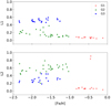 |
Fig. 7. L1 and L2 indices as a function of the metal content (Carretta et al. 2009). The different symbols and colours identify the different cluster groups defined in Milone et al. (2014): G1 (red crosses) for metal-rich globulars ([Fe/H] > −1.0), G2 (green triangles) for clusters with [Fe/H] < −1.0 and L1 ≤ 0.4, G3 (blue circles) for globulars with L1 ≥ 0.4. |
The data plotted in the top panel of this figure show that GGCs belonging to the G1 and the G2 groups display a steady increase of the L1 index when moving from metal-rich to metal-poor clusters. The G3 clusters attain an almost constant L1 value over more than 1 dex in metallicity. Moreover, a glance at the data shows that the standard deviation is modest, but the correlation does not seem to be mono-parametric. Indeed, there is evidence of metal-intermediate GGCs, mainly the G2 clusters, with the same metal content but with the L1 index changing by almost a factor of two. The data plotted in the bottom panel show that the L2 index does not show a correlation with the metal content (first parameter) and indeed metal-rich clusters (G1) display a modest extent in colour, while metal-intermediate and metal-poor (G2+G3) clusters cover a broad colour range. There are only two exceptions: NGC 6388 and NGC 6441, the two peculiar metal-rich globulars that host red HB and blue, extreme HB stars, plus RR Lyrae stars with unusually long periods (Pritzl et al. 2003). However, the data plotted in the bottom panel do not display any relevant correlation with the metal content.
Figure 8 (similar to Fig. 5 in Milone et al. 2014) shows the correlation between the new L1 (top panel) and L2 (bottom panel) indices and the homogeneous cluster age estimates provided by VandenBerg et al. (2013), Leaman et al. (2013). The data plotted in the top panel seem to suggest a possible mild correlation between the G2 clusters and the absolute age. On the other hand, the G1 and the G3 clusters do not show any significant correlation with cluster age. The data plotted in this diagram clearly show that GGCs with the same age have L1 indices that change by a factor of two or three. The data plotted in the bottom panel display that the L2 index is independent of cluster age. L2 index hardly changes inside the range in age covered by G1, G2 and G3 globulars. We performed the same analysis using the GCC ages provided by Salaris & Weiss (2002) and found similar trends. The reader interested in a more detailed analysis of the correlation between the L1/L2 indices and the GGC parameters is referred to Milone et al. (2014).
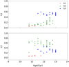 |
Fig. 8. L1 and L2 indices as a function of the cluster age (Gyr) from VandenBerg et al. (2013), Leaman et al. (2013). The different symbols and colours identify the different cluster groups defined in Milone et al. (2014): G1 (red crosses) for metal-rich globulars ([Fe/H] > −1.0), G2 (green triangles) for clusters with [Fe/H] < −1.0 and L1 ≤ 0.4, G3 (blue circles) for globulars with L1 ≥ 0.4. |
5. A new HB morphology index: τHB
To provide a new perspective on the investigation of the HB morphology and to overcome some of the limitations affecting the current HB morphology indices, we have devised a new parameter, christened τHB, based on the ratio of the areas subtended by the CNDs as a function of magnitude (I-band) and colour (V − I) of HB stars. To estimate the new HB morphology index first we defined a box in the I, V − I CMD large enough to include all cluster HB stars, independently of the HB morphology. Then for each cluster we computed the CND in both magnitude and in colour. The reference luminosity level we selected from the Harris catalogue is the V (HB), which is the mean visual magnitude of HB stars inside the RR Lyrae instability strip. This V magnitude was transformed into an I-band magnitude assuming a mean V − I colour for the RR Lyrae stars equal to 0.45 (Braga et al. 2016). To perform homogeneous star counts ranging from EHB to RHB stars, we defined a box covering 1.7 mag in V − I colour and 6.5 mag in I-band, which is 4.5 mag fainter and 2.0 mag brighter than the I-band HB luminosity level. Finally, the selected HB stars are sorted as a function of the I-band apparent magnitude and we cumulated the star counts starting from the faintest and reddest stars in the box.
The top panels of Fig. 9 display HB stars in the I, V − I CMD for three GGCs covering a broad range of iron abundances and HB morphologies. They are NGC 6341 ([Fe/H] = −2.25), with an HB dominated by hot and extreme blue HB stars, NGC 5272 ([Fe/H] = −1.50) with a HB that includes blue and red HB stars, as well as RR Lyrae stars, and finally NGC 104 ([Fe/H] = −0.76) which is characterized by a red HB morphology. The bottom panels of the same figure display the normalized I-band CNDs of the HB stars plotted in the top panel. The data plotted in these panels show that the area subtended by the three CNDs (ACND, shaded area) changes significantly when moving from an HB morphology dominated by hot and extreme HB stars, to a morphology dominated by red HB stars. We find a slightly constant decrease of the I-band ACND by a factor of ∼1.4 when moving from NGC 6341 (ACND(I) = 424.2) to NGC 5272 (ACND(I) = 336.6) to NGC 104 (ACND(I) = 217.9). A decrease on the order of approximately two when moving from an extreme blue HB morphology (NGC 6341) to a red one (NGC 104).
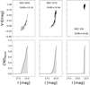 |
Fig. 9. Run of the normalized CND with respect to the I magnitude for three globular clusters (lower panels), chosen as representative of three different metallicity regimes (NGC 6341, NGC 5272, and NGC 104). Upper panels: horizontal branch of the three chosen globulars in I, V − I CMDs. |
Then, we sorted the HB stars located inside the box as a function of the (V − I) colour. The apparent colours were de-reddened using the colour excesses (E(B − V)) listed in Table 1. In this case the HB stars were counted starting from the reddest (coldest) HB stars. The top panels of Fig. 10 display HB stars in the I, V − I CMD for the same GGCs as in Fig. 9. The bottom panels display the normalized V − I CND of the HB stars plotted in the top panel. The shaded area shows a stronger sensitivity compared with the I-band ACND; indeed, they increase by almost a factor of three when moving from NGC 6341 (ACND(V − I) = 47.4) to NGC 5272 (ACND(V − I) = 81.5) and to NGC 104 (ACND(V − I)=137.9).
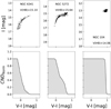 |
Fig. 10. Run of the normalized CND with respect to V − I for the same three globular clusters (lower panels) of Fig. 9. Upper panels: horizontal branch of the three chosen globulars in I, V − I CMDs. |
To estimate the CNDs in magnitude and in colour we accounted for the entire sample of HB stars, meaning stars located inside the RRL instability strip were included. The spread in magnitude and in colour of these objects is larger compared with typical HB stars. The difference is intrinsic, since we are using the mean of the measurements in both the V and the I band. In other words, we did not perform an analytical fit of the phased measurements.
To investigate the difference between the classical (HBR′) and the new (τHB) morphology index on a more quantitative basis, the left panel of Fig. 11 shows the comparison between the I-band ACND and the HBR′ index. The data plotted in this panel display a very well-defined linear correlation between I-band ACND and HBR′ index in the regime in which the latter attains intermediate values. The saturation for clusters dominated by blue HB morphologies (HBR′ ∼ 3) and red HB morphologies (HBR′ ∼ 1) is also quite clear at the top and the bottom of the panel. The right panel shows the same comparison as the left panel, but for the V − IACND. The data plotted in this panel show a linear anti-correlation over the entire range of values attained by the HBR′ index.
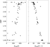 |
Fig. 11. Indices ACND(I) and ACND(V − I) vs. the HBR′ morphology index. |
We estimated the ratio between the area covered by the CND in magnitude and in colour, namely
 (3)
(3)
The V magnitude levels of the HB, which we transformed to I(HB) using the mean V − I of 0.45 mag, ACND(V − I), τHB, and their errors for the GGCs in our sample are listed in Cols. 10, 11, and 12 of Table 2, respectively. We propagated the error on τHB considering Poissonian uncertainties in the ACND.
Although τHB estimate is slightly more complex than the other indices presented in the literature, the new HB morphology index presents several key advantages compared with the classical HBR′ and L1/L2 indices:
Dynamical range. The current sample covers a range in τHB that is a factor of seven larger than the range covered by the HBR′ index. The data plotted in Fig. 12 show that when moving from metal-rich to less metal-rich GGCs (−1.0 < [Fe/H] < 0) the new index changes from zero to roughly three while the old one changes from one to roughly 1.5. The correlation between the old and new indices is linear in the metal intermediate regime, but it degenerates in the more metal-poor regime. Indeed, the τHB index increases by more than a factor of two (from six to fourteen), whereas the HBR′ takes on an almost constant value of three.
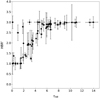 |
Fig. 12. Our new HB morphology index τHB vs. HBR′. |
The variation in τHB is a factor of twenty larger than the range covered by the L1 and L2 indices. The data plotted in Fig. 13 show that the G3 group is characterized by L1 values that are almost constant (L1 ∼ 0.5), while τHB changes from three to thirteen. The G1 and G2 groups display a mild linear correlation between L1 and τHB, but once again the variation in the L1 index is modest when compared with τHB index (0.3 vs. 7). The correlation between L2 and τHB is more noisy with a large spread at fixed τHB value.
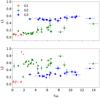 |
Fig. 13. L1 (top) and L2 (bottom) indices as a function of τHB for the globulars in our sample. The different symbols and colours identify the different cluster groups defined in Milone et al. (2014): G1 (red crosses) for metal-rich globulars ([Fe/H] > −1.0), G2 (green triangles) for clusters with [Fe/H] < −1.0 and L1 ≤ 0.4, G3 (blue circles) for globulars with L1 ≥ 0.4. |
Detailed sampling of the HB morphology. The CND in both magnitude and colour is sensitive to the star distribution along the HB. Data listed in Table 2 show that two metal-poor clusters, NGC 4833 and NGC 6341, with similar HBR′ (2.88 ± 0.07 vs. 2.92 ± 0.07) and L1 (0.287 ± 0.037 vs. 0.261 ± 0.075) indices, attain τHB values that differ at the 50% level (6.21 ± 0.21 vs. 8.95 ± 0.30). The same applies to metal-rich clusters, and indeed, two clusters like NGC 104 and NGC 6637 have the same HBR′ (1.01 ± 0.04 vs. 1.00 ± 0.09) and L1 (0.078 ± 0.005 vs. 0.078 ± 0.004) values, but the τHB value of the former cluster is a factor of three larger than the latter one (1.58 ± 0.01 vs. 0.54 ± 0.02). Data listed in Table 3 highlight several other pairs of GGCs characterized by a very similar iron content (Col. 2), HBR′ (Col. 3), and L14 (Col. 4) value, but quite different τHB values (Col. 5). The various pairs are separated in the table with horizontal lines.
Examples of globular pairs of similar metallicity and HBR′, but different values in τHB.
Global star count of HB stars. The τHB does not require any identification of specific subgroups (blue, red, variables).
6. Comparison between space- and ground-based data
As described in Sect. 2, when available we preferred the space-based observations for our analysis, while we used the ground-based data for the outer regions of the globulars in our sample. In this section, we analyse the HBR′ and τHB index evaluations using either ACS or ground-based observations, comparing them to the “global” index, which is the index estimated from both space- and ground-based data (see Sects. 3 and 5), giving higher priority to the first ones when both measures where available.
Figure 14 shows the relative difference between the HBR′ index estimated by using either ground-based (top panel) or ACS (bottom panel) data as a function of the global value listed in Col. 6 of Table 2. Data plotted in this figure show the following results. The top panel of Fig. 14 shows that the relative difference in HBR′ index from ground-based data is on average approximately 1.6%. The major exceptions are represented by the globulars NGC 1851 ( ) and NGC 7006 (
 ). The difference is mainly caused by the star counts of red HB stars (R) from ground-based observations. They provide a lower contribution when compared with space-based data (
 vs.
vs.  for the former cluster,
  vs.
vs.  for the latter one).
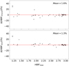 |
Fig. 14. Top: relative difference between the global HBR′ and the HBR′ values only based on ground-based data versus the global index. Note that in the estimate of the global index the priority in selecting the photometry was given to space-based (ACS at HST) data. Bottom: as the top panel, but the relative difference is between the global index and the HBR′ index only based on space-based data. The standard deviation of the estimates is represented by the error bar at the top left corner of the panels. At the top right corners we display the mean relative difference. |
The bottom panel shows that the difference in HBR′ index between  and
and  is on average ∼1.3%. It is marginally lower than the difference based on ground-based data. The single exception is NGC 6362, which is characterized by
  . Its global HBR′ index turns out to be redder than the ACS one (
 vs.
vs.  ) since in the global HBR′ estimate the contribution of red HB stars is mainly given by red HB stars from ground-based observations.
Figure 15 shows the global τHB index, evaluated in Sect. 5, versus the relative difference between the τHB index based either on ground-based (top panel) or on ACS (bottom panel) observations and the global one. A glance at the data plotted in this figure discloses a couple of interesting findings. The top panel shows that the relative difference in τHB index based on ground-based data shows a larger dispersion compared to that from space-based (bottom panel) data. The mean relative difference between τHB, Global and τHB, Ground is ∼3.6%. Moreover, thirteen globulars have a difference of |Δ(τHB, Ground)| greater than 20%. In this context it is worth mentioning that amongst them eleven are small, concentrated globulars. Indeed, their half-mass radius rh (Harris 1996) is entirely located inside the ACS FoV, namely NGC 1851 (23%, rh = 0.51′), NGC 2298 (24%, rh = 0.98′), NGC 5286 (32%, rh =0.73′), NGC 5986 (51%, rh = 0.98′), NGC 6681 (28%, rh =0.71′), NGC 6779 (24%, rh = 1.1′), NGC 6934 (25%, rh = 0.69′), NGC 7006 (71%, rh = 0.44′), NGC 7078 (66%, rh = 1.0′), Rup 106 (32%, rh = 1.05′), and Terzan 7 (29%, rh = 0.77′). This means that the main contribution in the τ index comes from space-based data, while ground-based data mainly contribute for HB stars located in the cluster outskirts. Two out of the thirteen globulars are larger, but located at large distances (true distance modulus DM ∼ 15 mag), namely NGC 288 (27%, rh = 2.23′) and NGC 5272 (27%, rh = 2.31′). This means that, even in these cases, most of the cluster stars are located inside the ACS FoV, giving a major contribution to the τHB, Global when compared to the ground-based observations.
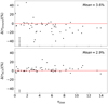 |
Fig. 15. Top: relative difference between the global τHB and the τHB index only based on ground-based data versus the global index. Note that in the estimate of the global index the priority in selecting stars was given to space-based (ACS at HST) data. Bottom: as the top panel, but the relative difference is between the global index and the τHB index only based on space-based data. The standard deviation of the estimates is represented by the error bar at the bottom left corner of the panels. At the top right corners we display the mean relative difference. |
The bottom panel shows that the relative variation between τHB, Global and τHB, ACS is, as expected low, on average 2.9%. The only exception is NGC 6717 (26%), in which ACS data do not populate the brighter region of the HB, giving a different estimate of τHB, ACS compared to the global one (5.61 vs. 4.46).
These findings support the fact that both ground-based and space observations of our sample of GGCs are statistically consistent and reliable. Moreover, our estimates of HBR′ and τHB are valid and well grounded: independently of the choice about the origin of the data they give the same results within a difference of at most 20% for τHB estimates.
The evidence of a larger relative difference in the τHB index shows that potentially our new index could quantify the different possible contribution to the HB morphology given by inner and outer populations within the globulars. This difference between star counts based on ground-based and on space-based data will be addressed in a future paper focused on the spectral energy distribution of Galactic globulars.
7. Correlation of τHB with cluster metallicity, age, and helium content
To investigate the correlation between τHB and fundamental cluster parameters, we study its relationship to cluster metallicity, absolute age, and internal spread in Helium abundance. Figure 16 shows τHB as a function of the iron content. The bulk of metal-poor GGCs ([Fe/H] ≤ −1.5) attains τHB values ranging from ∼9 to ∼4. In the metal-intermediate regime (−1.5 ≤ [Fe/H] ≤ −1.0) the bulk of the GGCs are characterized by τHB ranging from ∼5 to ∼2, while metal-rich clusters ([Fe/H] ≥ −1.0) attain τHB values smaller than 2 on average. There is a small sample of GGCs that attains τHB values that are, at fixed metal content, either systematically larger or systematically smaller than the typical ranges. To investigate on a more quantitative basis the identification of these GGCs, we performed a quadratic fit of the bulk of the GGCs. We found the best-fit function
![Mathematical equation: $$ \begin{aligned} \tau _{\rm HB}= 0.06-0.83\cdot \mathrm{[Fe/H]}+1.03\cdot \mathrm{[Fe/H]}^2, \end{aligned} $$](/articles/aa/full_html/2019/09/aa35995-19/aa35995-19-eq16.gif) (4)
(4)
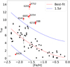 |
Fig. 16. Variation of τHB as a function of cluster metallicity (Carretta et al. 2009). The red line shows the quadratic best fit, the blue lines show 1.5σ levels. Red squares display the outliers, which are those objects located at more than 1.5σ from the quadratic fit. In the left corner the error bar shows the 0.1 dex error on the metal content. |
with a σ = 3.08 dispersion (see the red line in Fig. 16). We have defined as “outliers” the GGCs that attain, at fixed metal content, τHB values that are more than 1.5σ away from the best quadratic fit. We ended up with a subsample of seven metal-poor and metal-intermediate (−1.82 ≤ [Fe/H] ≤ −1.32) GGCs with τHB values larger than 9 (see red squares in Fig. 16). This subsample includes the GGCs that attain the largest τHB values, namely NGC 6205 (τHB = 13.37 ± 0.72) and NGC 6752 (τHB = 13.94 ± 0.78). This means that they are characterized by very blue HB morphologies. Data plotted in Fig. 16 also show a metal-poor GGC (NGC 6426) with τHB = 1.01 ± 0.16 that is a factor of four to ten smaller than the bulk of GGCs with similar metal abundances.
The above empirical evidence indicates that the new HB morphology index appears to be a solid diagnostic to select GGCs that are strongly affected by the second parameter problem. To further investigate the nature of these clusters we decided to perform a more detailed analysis of the GGCs in the metallicity range covered by the second parameter clusters. We selected three out of the eight outliers, namely NGC 6218 ([Fe/H] = −1.33, Age = 13 Gyr), NGC 6254 ([Fe/H] = −1.57, Age = 11.75 Gyr), and NGC 6541 ([Fe/H] = −1.82, Age = 12.50 Gyr), covering roughly 0.5 dex in metal content. The left panels of Fig. 17 show the I, V − I CMDs of these clusters. Assuming that the HB morphology is mainly driven by a difference in metal content, we selected three GGCs with iron abundances very similar to the selected outliers, but with τHB values close to the best-fit line plotted in Fig. 16, namely NGC 362 ([Fe/H] = −1.30, Age = 10.75 Gyr), NGC 6934 ([Fe/H] = −1.56, Age = 11.75 Gyr), and NGC 6144 ([Fe/H] = −1.82, Age = 12.75 Gyr). The right panels of Fig. 17 display their I, V − I CMDs. The CMDs display several interesting features worth discussing.
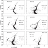 |
Fig. 17. CMDs (I, V − I) for three pairs of GGCs in the sample. Left panels: clusters belonging to the outlier group. Right panels: CMDs of clusters with similar [Fe/H] as the outlier ones, but following the main τHB-[Fe/H] relation. |
The top panels of Fig. 17 compare the CMDs of two metal-intermediate GGCs: an outlier cluster characterized by a very blue HB morphology, and a typical one (in terms of τHB, 9.05 vs. 3.24), mainly dominated by red HB stars. It is worth mentioning that the HB morphology of this pair of clusters could also be traced on the basis of the HBR′ index. Indeed, the HBR′ value of NGC 6218 is a factor of 2.5 larger than the HBR′ value of NGC 362.
The middle panels of Fig. 17 also display the CMDs of two metal-intermediate GGCs. The outlier GGC is characterized by a very blue HB morphology, while the typical one shows an HB that hosts variable stars, blue and red HB stars. For these GGCs the HBR′ index decreases by only the 30% when moving from NGC 6254 (3.00) to NGC 6934 (2.13). Interestingly enough, the τHB index differs by more than a factor of three.
The bottom panels of Fig. 17 display the CMDs of two metal-poor GGCs. The outlier GGC shows, as expected, a very blue HB morphology, while the “typical” one also shows a blue HB morphology. The HBR′ index for these two GGCs is identical within the errors: 2.99 for NGC 6541 and 3.00 for NGC 6144. On the other hand, the τHB index differs by more than a factor of two (10.26 vs. 4.98).
The current findings further support the strong sensitivity of the τHB index to variations in HB morphology when moving from the metal-intermediate to the metal-poor regime.
The anti-correlation found between the τHB index and the cluster metallicity does not include information about the cluster age. We have then investigated whether the new HB morphology index is correlated with the cluster ages.
To establish the age dependence we took advantage of the recent homogeneous age estimates provided by VandenBerg et al. (2013), Leaman et al. (2013). The data plotted in the top panel of Fig. 18 display a well-defined linear correlation between age and τHB. In particular, there is evidence that, when moving from a red to a blue HB morphology, GGCs become on average older. We performed a linear fit (τHB = a + b ⋅ Age, red line) whose coefficients are listed in Table 4, together with the standard deviation (σ). The dispersion around the linear fit is modest, equal to 1.21. However, the second parameter globulars identified in the τHB-[Fe/H] plane do not follow the same trend. They are on average more than 1.5σ away from the main relation, that is, at fixed cluster age their τHB values are systematically larger than typical GGCs. This further supports the evidence that the τHB index is a robust diagnostic to identify second parameter GGCs. It is worth mentioning the presence of four GGCs (NGC 6171, NGC 6362, NGC 6535, and NGC 7089) that are ∼2.5σ away from the linear fit, but their position might also be affected by uncertainties in the absolute cluster age (see the horizontal error bar plotted in the bottom right corner).
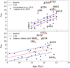 |
Fig. 18. Our index τHB as a function of cluster ages obtained from different authors. Top: cluster ages from VandenBerg et al. (2013), Leaman et al. (2013). The error bar in the lower left corner shows the conservative ±0.5 Gyr error on the GGC ages. Bottom: ages from Salaris & Weiss (2002) based on the metallicity scale provided by Carretta & Gratton (1997). In both panels red squares are the same second parameter clusters shown in Fig. 16 and discussed in this section. Red lines determine the best-fit to each data sample, blue lines the ±1σ levels. |
Best fit parameters for the linear functions fitting the τHB-Age relations used in this work.
To further investigate the impact of possible systematics on the cluster ages, we used the results by Salaris & Weiss (2002) employing the Carretta & Gratton (1997) metallicity scale, for their 43 GGCs in common with our sample. They divided the sample into four different metallicity bins and for each of them selected a calibrating cluster. They then estimated the absolute age of the calibrating cluster by using the vertical method, that is, the difference in visual magnitude (ΔV) between the HB luminosity level and the MSTO. For all the other clusters in a specific metallicity bin, they estimated the relative age with respect to the calibrating cluster by using the horizontal method, that is, the difference in colour (Δ(V − I) or Δ(B − V)) between the main sequence TO and the base of the RGB.
Data are shown in the bottom panel of Fig. 18. Once again, we found that the τHB index correlates with the cluster age. We performed the same linear fit as for the age estimates by VandenBerg et al. (2013), Leaman et al. (2013), and the coefficients are listed in Table 4 together with the standard deviation, which is equal to 1.89. The red and the blue lines display the linear fit and the 1σ limits, respectively. The difference between the second parameter clusters and the linear fit is larger than 2σ. This means that their peculiarity is independent of the adopted absolute age. Moreover, this plot also shows a few GGCs, roughly 2σ away from the linear fit, already identified in the top panels: NGC 6171 and NGC 6535, plus a new one, NGC 6652.
We analysed the age and the metallicity dependencies of τHB, since they are considered as the main culprits affecting the HB morphology. However, the current findings further support the need for at least one more parameter to explain the observed variation in HB morphology. We assumed as a working hypothesis that the dispersion in the τHB-age diagram was caused by both age and helium variations (D’Antona et al. 2002; Caloi & D’Antona 2005). Therefore, we decided to empirically remove the age dependence of τHB, and check whether the residuals in the reduced τHB-[Fe/H] diagram correlate with the spread in helium of the cluster. This empirical “reduction” of τHB to a single age accounts automatically for possible age-metallicity relations in the cluster sample, as well as for the dependence of τHB on age at fixed metallicity. To perform this experiment we reduced the individual τHB measurements (Table 2) to the values they would have for an age of 12 Gyr (τHB, 12 Gyr, using the ages by VandenBerg et al. 2013), as detailed below.
We first calculated the index value at an age of 12 Gyr as provided by the best-fit relation in the upper panel of Fig. 18 (value equal to 4.63); then, for each cluster, we calculated the values determined from the same best-fit relation but for the individual cluster ages. For each GGC we then calculated the difference dτ between the value expected at the cluster age and the value expected at 12 Gyr, and finally determined τHB, 12 Gyr = τHB − dτ.
Figure 19 shows the τHB, 12 Gyr values as a function of [Fe/H]. In contrast to what we found in Fig. 16, after eliminating on average the effect of age, we now have a linear best-fit relation between τHB, 12 Gyr and the metal content (the red line in Fig. 19):
![Mathematical equation: $$ \begin{aligned} \tau _{\rm HB, 12\,Gyr}=3.02-0.89\cdot \mathrm{[Fe/H]}, \end{aligned} $$](/articles/aa/full_html/2019/09/aa35995-19/aa35995-19-eq17.gif) (5)
(5)
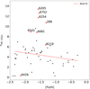 |
Fig. 19. [Fe/H] vs. τHB, 12 Gyr. The red line identifies the linear best-fit function of the plane, and red squares mark the eight second parameter clusters (see text for details). |
with dispersion σ = 1.64. The red squares identify the second parameter clusters: they still attain τHB, 12 Gyr values far from the best-fit relation.
In a very recent paper, Milone et al. (2018) estimated the spread in initial helium content (0.245 ≤ Y ≤ 0.4) for a sizeable sample of GGCs (57). They used data from the HST UV survey of Galactic GCs (F275W, F336W, and F438W filters of the ultraviolet and visual channel of HST/WFC3 (UVIS/WFC3), Piotto et al. 2015; Milone et al. 2017) and from the Wide Field Channel of the Advanced Camera for Surveys (WFC/ACS) (F606W and F814W photometry, Sarajedini et al. 2007; Dotter et al. 2011) programmes. The He spread values, ∂Ymax, for each of the 56 GGCs in common with Milone et al. (2018) are listed in Col. 9 of Table 2.
The spread in helium content ranges from almost zero for NGC 6362, NGC 6535, and NGC 6717, up to ∼0.08 for NGC 6388, NGC 6441, and NGC 7078. To further constrain the sensitivity of the new HB morphology index, we correlated the residuals of τHB, 12 Gyr of the best-fit function in Fig. 19 as a function of the metallicity, shown in Fig. 20.
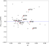 |
Fig. 20. Residuals of the corrected τHB, 12 Gyr as a function of the metal content (Carretta et al. 2009) versus the spread in helium content ∂Y estimated by Milone et al. (2018). Red squares identify the second parameter globulars. |
The figure shows that the τHB, 12 Gyr index does not seem to be correlated with the spread in helium content. This means that, despite our attempt to limit the age and metallicity effects, the spread in helium content is not able to justify the observed spread in τHB. We note that we also estimated the residuals of the τHB, 12 Gyr using just space data (see Sect. 6) and related them to ∂Y values, since the latter quantities are evaluated from the same HST data. Once again, despite the data homogeneity, we did not find any clear correlation with ∂Y values.
8. Comparison with synthetic horizontal branch models
To constrain on a more quantitative basis the impact that both cluster age and spread in helium content have on the observed spread of the new HB morphology index, we decided to use a novel set of synthetic horizontal branch (SHB) models. The synthetic HB models have been computed employing HB tracks and progenitor isochrones from the α-enhanced a Bag of Stellar Tracks and Isochrones (BaSTI) stellar model library (Pietrinferni et al. 2006)5 and a code fully described in Dalessandro et al. (2013). We considered three different metallicities, namely [Fe/H] = −0.7, [Fe/H] = −1.62, and [Fe/H] = −2.14 (all with [α/Fe] = 0.4). The initial He abundances of the HB progenitors at these three metallicities are equal to Y = 0.245, 0.246, and 0.256, respectively.
For each [Fe/H] we calculated first a set of synthetic HBs for an age equal to 12 Gyr (keeping Y constant for each [Fe/H]), assuming the RGB progenitor loses an amount of mass ΔM = 0.28 M⊙, ΔM = 0.21 M⊙, and ΔM = 0.16 M⊙ for Fe/H] = −0.7, [Fe/H] = −1.62, and [Fe/H] = −2.14, respectively. The mass loss is estimated with a 1σ Gaussian spread equal to 0.01 M⊙, irrespective of the chemical composition. In addition, assuming the same age and RGB mass loss, we calculated SHBs for each metallicity with an uniform distribution of initial Y for the progenitors, with a range ∂Y = 0.03.
In brief, the synthetic HB code first draws randomly a value of Y with a uniform probability distribution between Y and Y + ∂Y (∂Y = 0 for the models at constant He) and determines the initial mass of the star at the RGB tip (MTRGB) from interpolation amongst the BaSTI isochrones of the chosen age. The mass of the corresponding object evolving along the HB (MHB) is then calculated as MHB = MTRGB − ΔM, where ΔM is drawn randomly according to a Gaussian distribution with the specified mean values and σ. The magnitudes of the synthetic star are then determined according to its position along the HB track with appropriate mass and Y obtained by interpolation among the available set of HB tracks, after an evolutionary time t has been randomly extracted. The value of t is determined assuming that stars reach the ZAHB at a constant rate, employing a flat probability distribution ranging from zero to tHB, where tHB is the time spent from the ZAHB to the He-burning shell ignition along the early asymptotic giant branch. The value of tHB is set by the HB mass with the longest lifetime (the lowest masses for a given chemical composition). This implies that for some objects the randomly selected value of t will be longer than its tHB, meaning that they have already evolved to the next evolutionary stages.
Figure 21 shows the comparison between the τHB, 12 Gyr morphology index as a function of cluster iron abundance, and synthetic horizontal branch models. The blue line shows the SHB model at constant helium content (∂Y = 0), while the black one is the synthetic model constructed assuming an internal spread in He content of ∂Y = 0.03. This value was adopted according to the recent estimates provided by Milone et al. (2018).
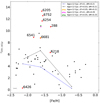 |
Fig. 21. New HB morphology index, τHB, 12 Gyr, as a function of cluster iron abundance (Carretta et al. 2009). The two lines display synthetic HB models at fixed cluster age (12 Gyr), but either with a canonical helium content (∂Y = 0, blue line) or with an internal spread in He of ∂Y = 0.03 (black line). The coloured triangles identify three models for [Fe/H] = −1.6 for three different combinations of ∂Y and ΔM (see legend). Red squares mark the eight second parameter clusters. The error bar on the left corner gives the 0.1 dex error on the metal content. |
In the metal-rich regime ([Fe/H] ≥ −0.7) the predicted τHB weakly changes with the spread in helium content. This is a consequence of the fact that SHB models predict an extreme red HB morphology, minimally affected by the intrinsic parameters we are taking into account. In the metal-intermediate regime ([Fe/H] = −1.62) the τHB value predicted assuming an internal spread ∂Y is characterized by a spike. This is due to the fact that at this metallicity values, a small mass variation causes significant changes in the SHB colour.
To explain the existence of our second parameter clusters, the triangles in Fig. 21 identify a further three different synthetic models for [Fe/H] = −1.6, the mean metallicity value of our second parameter clusters, at the fixed age of 12 Gyr. The yellow triangle shows the synthetic τHB considering a higher spread in He compared to the one estimated by Milone et al. (2018) (∂Y = 0.05) at the mass loss value we used for the blue and black models (ΔM = 0.21); the magenta triangle identifies the model for ∂Y = 0 and a mass loss of ΔM = 0.29 (higher of 0.08 M⊙ than the standard one); finally the green triangle identifies the synthetic τHB value for the case with ∂Y = 0.05 and ΔM = 0.25.
Therefore, Fig. 21 shows that if we want to model the estimated values of τHB, 12 Gyr we have three different possibilities. If we adopt the spread in He content estimated by Milone et al. (2018) (e.g. ∂Y = 0.05 for NGC 6205, ∂Y = 0.04 for NGC 6752, ∂Y = 0.03 for NGC 6254, ∂Y = 0.03 for NGC 6681, considering the second parameter cluster with [Fe/H] ∼ −1.6), we need to increase the mass loss value to 0.29, which is a value greater by 0.08 M⊙ than the one able to fit the bulk of the clusters. If we fix the mass loss to the one needed to model the bulk of the clusters (ΔM = 0.21), then we need to increase the spread in He content (from ∂Y = 0.03 to, at least, ∂Y = 0.05). Finally, we can explain the existence of the second parameter cluster also considering a higher mass loss together with a higher spread in He. We note that the adoption of a higher mass loss cannot be attributed to systematic errors in age estimations, since they should be on the order of 2−3 Gyr.
9. Conclusions
We took advantage of a sample of 64 GGCs for which we have homogeneous and accurate UBVRI ground photometry and V (F606W), I (F814W) ACS/HST data (Sarajedini et al. 2007; Dotter et al. 2011), to introduce a new HB morphology index, named τHB, to investigate on a more quantitative basis the variation of the HB morphology when moving from the metal-poor to the metal-rich regime. We define τHB as the ratio of the area below the cumulative number distribution in apparent magnitude (ACND(I)) and in colour (ACND(V − I)) of the entire HB region.
Even though the estimate of the τHB index appears to be more complicated compared with HB morphology indices based either on star counts (HBR′, Lee et al. 1990) or on specific evolutionary features (L1, L2, Milone et al. 2014), it offers several advantages. Indeed, we found that τHB is a factor of seven more sensitive than the classical HBR′ index and more than one order of magnitude more sensitive compared to L1 or L2 indices. Moreover, and even more importantly, the τHB index shows a linear trend over the entire metallicity range (−2.35 ≤ [Fe/H] ≤ −0.12) covered by GGCs. Furthermore, the τHB index traces the HB luminosity function and it is independent of uncertainties affecting either the definition of different sub-groups (blue, red, variables) or the position of specific evolutionary features (L1, L2).
Moreover, to analyse the possible sensitivity of the HB morphology indices to the different contribution of inner and outer populations in GGCs, we estimated HBR′ and τHB considering just space-based and just ground-based data. Comparing them to the results obtained using the combined HST and ground-based observations, we found that HBR′ has on average lower differences (∼1.6%, just ground-based, and ∼1.3%, just space-based) than the ones attained by τHB (∼3.6%, just ground-based, and ∼2.9%, just space-based). For HBR′ we observed major differences for the globulars in which the contribution of the red HB stars is mainly driven by HST observations. In τHB analysis we found higher differences for small and concentrated clusters, or for those clusters which are larger but located at higher distances. In all these cases most of the cluster stars are located inside the ACS FoV and so the space-based data give the higher contribution to the global τHB. In general our data are self-consistent and reliable and τHB higher relative differences could mean that it is sensitive to the different contribution given by inner and outer populations observed in GGCs.
To quantify the sensitivity of the τHB index on intrinsic stellar parameters, we investigated its dependence on cluster global properties (metallicity, absolute age, spread in He content). The main results of our analysis are the following:
Anti-correlation with cluster metallicity. We found a quadratic anti-correlation between τHB and [Fe/H]. The majority of the metal-poor globulars ([Fe/H] ≤ −1.5) have τHB between ∼4 and ∼9, while the metal-intermediate ones (−1.5 ≤ [Fe/H] ≤ −1.0) have values between ∼2 and ∼5. On the other hand, the metal-rich clusters, with [Fe/H] ≥ −1.0, attain τHB values smaller than two.
Identification of second parameter clusters. We found a subsample of eight GGCs in the metal-poor and metal-intermediate regime (−1.82 ≤ [Fe/H] ≤ −1.32) which, at fixed metallicity, are characterized by τHB values that are, on average, at least a factor of two larger than canonical clusters. The outlier clusters do not display any peculiarity in the HBR′ metallicity plane. To investigate their HB morphology, we selected three of them that sample the metal-rich ([Fe/H] = −1.33, NGC 6218), metal-intermediate ([Fe/H] = −1.57, NGC 6254), and metal-poor ([Fe/H] = −1.82, NGC 6541) regimes. We compared their I, V − I CMDs to those of three “regular” clusters with similar metallicities within the errors (NGC 362, NGC 6934, and NGC 6144). For each cluster pair, we find similar HBR′ values but different τHB values, with differences even on the order of three. For these reasons we can associate these clusters in our sample with the so-called second parameter clusters.
Correlation with cluster age. We investigate the relation between our HB morphology index τHB and the absolute cluster age. To exclude possible dependence on the particular age estimation, we used the different homogeneous evaluations from VandenBerg et al. (2013), Leaman et al. (2013), Salaris & Weiss (2002), finding a linear correlation between τHB and the absolute age. We found that, in general, when moving from red to blue HB morphology, the GGCs become older. The second parameter clusters selected according to the τHB-metallicity plane appear to be peculiar also in the τHB-absolute age plane. In particular they attain cluster ages ranging from ∼11.5 to ∼13 Gyr. Moreover, they seem to be characterized by bluer HB morphologies than the typical clusters.
Reductio ad unum. We limited the age impact on our analysis by reducing the τHB values to the ones they would attain for an age of 12 Gyr. In contrast to what we originally found, we found a linear correlation between the corrected τHB, 12 Gyr values and [Fe/H]. However, the second parameter clusters are still located far from the best-fit linear relation of the plane.
Comparison with spread in helium content. We investigated our new HB morphology index in the context of internal helium content variation, supposed to be one of the main drivers of the HB morphology. We compared the residuals of the corrected τHB, 12 Gyr as a function of cluster metallicity with the internal spread in helium content, ∂Y, estimated by Milone et al. (2018), but we did not find a solid correlation.
Comparison with theory. We calculated a novel set of synthetic horizontal branch models to investigate the impact on τHB of the spread in Helium content and mass loss along the branch, at the fixed age of 12 Gyr. We found that we can fit the second parameter clusters in our sample if: we fix the spread in He content to the one estimated by Milone et al. (2018) and we increase the mass loss value from ΔM = 0.21 (the one able to fit the bulk of the clusters) to ΔM = 0.29; we fix the mass loss to ΔM = 0.21 and we increase the spread in He content from ∂Y = 0.03 (Milone et al. 2018) to, at least, ∂Y = 0.05; we consider a higher mass loss together with an higher spread in He content.
Nature versus nurture. It is not clear whether the outlier clusters display a bluer HB morphology because they are intrinsically different (nature) or because the HB morphology is tracing a specific dynamical status of the cluster (nurture).
Photometry available at https://www.astro.ufl.edu/~ata/public_hstgc/
We did not consider L2 since it does not correlate with age, metallicity, and τHB.
Acknowledgments
This work has made use of data from An ACS Survey of Galactic Globular Clusters programme in the context of the Hubble Space Telescope Treasury project. This investigation was partially supported by PRIN-INAF 2016 ACDC (P.I.:P. Caraveo). M.M. was supported by the Spanish Ministry of Economy and Competitiveness (MINECO) under the grant AYA2017-89076-P.
References
- Anderson, J., Sarajedini, A., Bedin, L. R., et al. 2008, AJ, 135, 2055 [NASA ADS] [CrossRef] [Google Scholar]
- Bono, G., & Stellingwerf, R. F. 1994, ApJS, 93, 233 [NASA ADS] [CrossRef] [Google Scholar]
- Bono, G., Marconi, M., & Stellingwerf, R. F. 1999, ApJS, 122, 167 [NASA ADS] [CrossRef] [Google Scholar]
- Braga, V. F., Stetson, P. B., Bono, G., et al. 2016, AJ, 152, 170 [NASA ADS] [CrossRef] [Google Scholar]
- Brown, T. M., Sweigart, A. V., Lanz, T., et al. 2010, ApJ, 718, 1332 [NASA ADS] [CrossRef] [Google Scholar]
- Buonanno, R. 1993, in The Globular Cluster-Galaxy Connection, eds. G. H. Smith, & J. P. Brodie, ASP Conf. Ser., 48, 131 [NASA ADS] [Google Scholar]
- Calamida, A., Strampelli, G., Rest, A., et al. 2017, AJ, 153, 175 [NASA ADS] [CrossRef] [Google Scholar]
- Caloi, V., & D’Antona, F. 2005, A&A, 435, 987 [NASA ADS] [CrossRef] [EDP Sciences] [Google Scholar]
- Carretta, E., & Gratton, R. G. 1997, A&AS, 121, 95 [NASA ADS] [CrossRef] [EDP Sciences] [Google Scholar]
- Carretta, E., Bragaglia, A., Gratton, R., D’Orazi, V., & Lucatello, S. 2009, A&A, 508, 695 [NASA ADS] [CrossRef] [EDP Sciences] [Google Scholar]
- Carretta, E., Bragaglia, A., Gratton, R. G., et al. 2014, A&A, 564, A60 [NASA ADS] [CrossRef] [EDP Sciences] [Google Scholar]
- Castellani, M., Caputo, F., & Castellani, V. 2003, A&A, 410, 871 [NASA ADS] [CrossRef] [EDP Sciences] [Google Scholar]
- Chaboyer, B., McArthur, B. E., O’Malley, E., et al. 2017, ApJ, 835, 152 [NASA ADS] [CrossRef] [Google Scholar]
- Clement, C. M., Muzzin, A., Dufton, Q., et al. 2001, AJ, 122, 2587 [NASA ADS] [CrossRef] [Google Scholar]
- Dalessandro, E., Salaris, M., Ferraro, F. R., Mucciarelli, A., & Cassisi, S. 2013, MNRAS, 430, 459 [NASA ADS] [CrossRef] [Google Scholar]
- D’Antona, F., Caloi, V., Montalbán, J., Ventura, P., & Gratton, R. 2002, A&A, 395, 69 [NASA ADS] [CrossRef] [EDP Sciences] [Google Scholar]
- Di Cecco, A., Bono, G., Prada Moroni, P. G., et al. 2015, AJ, 150, 51 [NASA ADS] [CrossRef] [Google Scholar]
- D’Orazi, V., Magurno, D., Bono, G., et al. 2018, ApJ, 855, L9 [NASA ADS] [CrossRef] [Google Scholar]
- Dotter, A., Chaboyer, B., Jevremović, D., et al. 2007, AJ, 134, 376 [NASA ADS] [CrossRef] [Google Scholar]
- Dotter, A., Sarajedini, A., & Anderson, J. 2011, ApJ, 738, 74 [NASA ADS] [CrossRef] [Google Scholar]
- Dutra, C. M., & Bica, E. 2000, A&A, 359, 347 [NASA ADS] [Google Scholar]
- Freeman, K. C., & Norris, J. 1981, ARA&A, 19, 319 [NASA ADS] [CrossRef] [Google Scholar]
- Gratton, R. G., Carretta, E., Bragaglia, A., Lucatello, S., & D’Orazi, V. 2010, A&A, 517, A81 [NASA ADS] [CrossRef] [EDP Sciences] [Google Scholar]
- Harris, W. E. 1996, AJ, 112, 1487 [NASA ADS] [CrossRef] [Google Scholar]
- Iannicola, G., Monelli, M., Bono, G., et al. 2009, ApJ, 696, L120 [NASA ADS] [CrossRef] [Google Scholar]
- Kraft, R. P., & Ivans, I. I. 2003, PASP, 115, 143 [NASA ADS] [CrossRef] [Google Scholar]
- Lanzoni, B., Ferraro, F. R., Mucciarelli, A., et al. 2018, ApJ, 861, 16 [NASA ADS] [CrossRef] [Google Scholar]
- Leaman, R., VandenBerg, D. A., & Mendel, J. T. 2013, MNRAS, 436, 122 [NASA ADS] [CrossRef] [Google Scholar]
- Lee, Y. W. 1989, PhD Thesis, Yale University [Google Scholar]
- Lee, Y.-W., Demarque, P., & Zinn, R. 1990, ApJ, 350, 155 [NASA ADS] [CrossRef] [Google Scholar]
- Lee, Y.-W., Demarque, P., & Zinn, R. 1994, ApJ, 423, 248 [NASA ADS] [CrossRef] [Google Scholar]
- Marconi, M., Coppola, G., Bono, G., et al. 2015, ApJ, 808, 50 [NASA ADS] [CrossRef] [Google Scholar]
- Milone, A. P., Marino, A. F., Dotter, A., et al. 2014, ApJ, 785, 21 [NASA ADS] [CrossRef] [Google Scholar]
- Milone, A. P., Piotto, G., Renzini, A., et al. 2017, MNRAS, 464, 3636 [NASA ADS] [CrossRef] [Google Scholar]
- Milone, A. P., Marino, A. F., Renzini, A., et al. 2018, MNRAS, 481, 5098 [NASA ADS] [CrossRef] [Google Scholar]
- Monelli, M., Testa, V., Bono, G., et al. 2015, ApJ, 812, 25 [NASA ADS] [CrossRef] [Google Scholar]
- Pancino, E., Galfo, A., Ferraro, F. R., & Bellazzini, M. 2007, ApJ, 661, L155 [NASA ADS] [CrossRef] [Google Scholar]
- Pietrinferni, A., Cassisi, S., Salaris, M., & Castelli, F. 2006, ApJ, 642, 797 [NASA ADS] [CrossRef] [Google Scholar]
- Piotto, G., Milone, A. P., Bedin, L. R., et al. 2015, AJ, 149, 91 [NASA ADS] [CrossRef] [Google Scholar]
- Pritzl, B. J., Smith, H. A., Stetson, P. B., et al. 2003, AJ, 126, 1381 [NASA ADS] [CrossRef] [Google Scholar]
- Recio-Blanco, A., Aparicio, A., Piotto, G., de Angeli, F., & Djorgovski, S. G. 2006, A&A, 452, 875 [NASA ADS] [CrossRef] [EDP Sciences] [Google Scholar]
- Richer, H. B., Goldsbury, R., Heyl, J., et al. 2013, ApJ, 778, 104 [NASA ADS] [CrossRef] [Google Scholar]
- Salaris, M., & Weiss, A. 2002, A&A, 388, 492 [NASA ADS] [CrossRef] [EDP Sciences] [Google Scholar]
- Salaris, M., & Cassisi, S. 2005, Evolution of Stars and Stellar Populations (Wiley) [CrossRef] [Google Scholar]
- Sandage, A. R. 1953, AJ, 58, 61 [NASA ADS] [CrossRef] [Google Scholar]
- Sandage, A., & Wildey, R. 1967, ApJ, 150, 469 [NASA ADS] [CrossRef] [Google Scholar]
- Sarajedini, A., Bedin, L. R., Chaboyer, B., et al. 2007, AJ, 133, 1658 [NASA ADS] [CrossRef] [Google Scholar]
- Searle, L., & Zinn, R. 1978, ApJ, 225, 357 [NASA ADS] [CrossRef] [Google Scholar]
- Stetson, P. B., Catelan, M., & Smith, H. A. 2005, PASP, 117, 1325 [NASA ADS] [CrossRef] [Google Scholar]
- Stetson, P. B., Braga, V. F., Dall’Ora, M., et al. 2014, PASP, 126, 521 [NASA ADS] [CrossRef] [Google Scholar]
- Stetson, P. B., Pancino, E., Zocchi, A., Sanna, N., & Monelli, M. 2019, MNRAS, 485, 3042 [NASA ADS] [CrossRef] [Google Scholar]
- van den Bergh, S. 1967, AJ, 72, 70 [NASA ADS] [CrossRef] [Google Scholar]
- VandenBerg, D. A., Brogaard, K., Leaman, R., & Casagrande, L. 2013, ApJ, 775, 134 [NASA ADS] [CrossRef] [Google Scholar]
- Villanova, S., Geisler, D., Piotto, G., & Gratton, R. G. 2012, ApJ, 748, 62 [NASA ADS] [CrossRef] [Google Scholar]
- Weiss, A., Schlattl, H., Salaris, M., & Cassisi, S. 2004, A&A, 422, 217 [NASA ADS] [CrossRef] [EDP Sciences] [Google Scholar]
- Zinn, R., & West, M. J. 1984, ApJS, 55, 45 [NASA ADS] [CrossRef] [Google Scholar]
- Zoccali, M., Cassisi, S., Bono, G., et al. 2000, ApJ, 538, 289 [NASA ADS] [CrossRef] [Google Scholar]
- Zocchi, A., Gieles, M., & Hénault-Brunet, V. 2017, MNRAS, 468, 4429 [NASA ADS] [CrossRef] [Google Scholar]
Appendix A: Peculiar globular clusters
The classical HB morphology index (HBR′) estimations for NGC 6304, NGC 6426, NGC 6624, Lynga 7, and Palomar 2 and the τHB indices for NGC 6426, NGC 6624, and NGC 6652 were derived using I, V-bands from ACS-HST because we lack ground-based catalogues. For these globulars we considered all the stars in the HST field and within the tidal radius in ground-based telescope fields.
Due to the high field contamination in ground observations, for the clusters NGC 6388 and NGC 6441, we used only ACS data. Despite this, the sample is statistically good enough to analyse their HB morphology, even if the ACS FoV does not cover the entire extent of these two clusters.
Owing to the low number of HB stars in Lynga 7 and NGC 6304, we obtain τHB = 0 and so, these clusters have not been included in the analysis of our new index. Finally, we note that ground-based data for NGC 104, NGC 5272, NGC 5466, NGC 5927, NGC 6362, NGC 6397, and NGC 6752 do not reach the tidal radius.
Appendix B: Notes on individual outliers
In the following we give notes about the clusters we can define as outliers either in the τHB-[Fe/H] plane or in the τHB-age plane or both.
NGC 6218. Outlier of τHB-[Fe/H], while we cannot consider it an outlier in τHB-age planes (it is located under the 2.0σ levels). Both ground-based and space data are of good quality. It has been identified as a second parameter cluster.
NGC 288. Outlier of τHB-[Fe/H] and of the τHB-age planes. Both ground-based and space data are of good quality. It has been identified as a second parameter cluster.
NGC 6205. Outlier of τHB-[Fe/H] and of the τHB-age planes. Both ground-based and space data are of good quality. It has been identified as a second parameter cluster.
NGC 6254. Outlier of τHB-[Fe/H] and of the τHB-age planes. Both ground-based and space data are of good quality. It has been identified as a second parameter cluster.
NGC 6426. Outlier of τHB-[Fe/H] and of τHB-age planes. We have only space photometry. Among the second parameter clusters, it is the one attaining the lowest value in τHB.
NGC 6752. Outlier of τHB-[Fe/H] and of the τHB-age planes. Both ground-based and space data are of good quality, but ground data do not reach the globular tidal radius. It has been identified as a second parameter cluster.
NGC 6541. Outlier of τHB-[Fe/H] and of the VandenBerg et al. (2013), Leaman et al. (2013)τHB-age plane. We have no age estimation from Salaris & Weiss (2002). Both ground-based and space data are of good quality. It has been identified as a second parameter cluster.
NGC 6681. Outlier of τHB-[Fe/H] and of the τHB-age planes. Both ground-based and space data are of good quality. It has been identified as a second parameter cluster.
NGC 6362. Outlier of τHB-age plane for age estimations from VandenBerg et al. (2013), Leaman et al. (2013). Both ground-based and space data are of good quality.
NGC 6535. Outlier of τHB-age planes (above 2.5σ limit in the VandenBerg et al. 2013; Leaman et al. 2013 plane and 2.0σ limit in the Salaris & Weiss 2002 one). Both ground-based and space data are of good quality.
NGC 6652. Outlier of the Salaris & Weiss (2002)τHB-age plane. Both ground-based and space data are of good quality.
NGC 7089. Outlier of the VandenBerg et al. (2013), Leaman et al. (2013)τHB-age plane. We have no age estimation from Salaris & Weiss (2002). Both ground-based and space data are of good quality.
NGC 6171. Outlier in the τHB-age planes (above the 2.5σ limit in VandenBerg et al. 2013 and the 2.0σ limit in Salaris & Weiss 2002). Both ground-based and space data are of good quality.
All Tables
Examples of globular pairs of similar metallicity and HBR′, but different values in τHB.
Best fit parameters for the linear functions fitting the τHB-Age relations used in this work.
All Figures
|
Fig. 1. Sky distribution of ground-based (black dots) and space-based (red dots) data for the cluster NGC 5053. North is up and east is to the left. |
| In the text | |
|
Fig. 2. Cluster NGC 5286 I, V − I CMD based only on ACS-HST data. |
| In the text | |
|
Fig. 3. Cluster NGC 5286 V, B − I CMD. Left panel: all stars. Central panel: our candidate cluster stars. Right panel: candidate field stars. Candidate cluster and field stars have been selected following the method described in the main text. |
| In the text | |
|
Fig. 4. Difference between Harris (1996) values (2003 version) for HBR and our measurements as a function of [Fe/H]. |
| In the text | |
|
Fig. 5. Observed HBR′ values as a function of metal content. The metallicity scale is from Carretta et al. (2009) (see the appendix for more details). The error bar in the lower left corner gives the uncertainty of the metal content (0.1 dex). |
| In the text | |
|
Fig. 6. Observed HBR′ values as a function of the cluster ages (gigayears (Gyr)) provided by VandenBerg et al. (2013), Leaman et al. (2013). The error bar in the lower left corner gives the uncertainty in the cluster ages (±0.5 Gyr). |
| In the text | |
|
Fig. 7. L1 and L2 indices as a function of the metal content (Carretta et al. 2009). The different symbols and colours identify the different cluster groups defined in Milone et al. (2014): G1 (red crosses) for metal-rich globulars ([Fe/H] > −1.0), G2 (green triangles) for clusters with [Fe/H] < −1.0 and L1 ≤ 0.4, G3 (blue circles) for globulars with L1 ≥ 0.4. |
| In the text | |
|
Fig. 8. L1 and L2 indices as a function of the cluster age (Gyr) from VandenBerg et al. (2013), Leaman et al. (2013). The different symbols and colours identify the different cluster groups defined in Milone et al. (2014): G1 (red crosses) for metal-rich globulars ([Fe/H] > −1.0), G2 (green triangles) for clusters with [Fe/H] < −1.0 and L1 ≤ 0.4, G3 (blue circles) for globulars with L1 ≥ 0.4. |
| In the text | |
|
Fig. 9. Run of the normalized CND with respect to the I magnitude for three globular clusters (lower panels), chosen as representative of three different metallicity regimes (NGC 6341, NGC 5272, and NGC 104). Upper panels: horizontal branch of the three chosen globulars in I, V − I CMDs. |
| In the text | |
|
Fig. 10. Run of the normalized CND with respect to V − I for the same three globular clusters (lower panels) of Fig. 9. Upper panels: horizontal branch of the three chosen globulars in I, V − I CMDs. |
| In the text | |
|
Fig. 11. Indices ACND(I) and ACND(V − I) vs. the HBR′ morphology index. |
| In the text | |
|
Fig. 12. Our new HB morphology index τHB vs. HBR′. |
| In the text | |
|
Fig. 13. L1 (top) and L2 (bottom) indices as a function of τHB for the globulars in our sample. The different symbols and colours identify the different cluster groups defined in Milone et al. (2014): G1 (red crosses) for metal-rich globulars ([Fe/H] > −1.0), G2 (green triangles) for clusters with [Fe/H] < −1.0 and L1 ≤ 0.4, G3 (blue circles) for globulars with L1 ≥ 0.4. |
| In the text | |
|
Fig. 14. Top: relative difference between the global HBR′ and the HBR′ values only based on ground-based data versus the global index. Note that in the estimate of the global index the priority in selecting the photometry was given to space-based (ACS at HST) data. Bottom: as the top panel, but the relative difference is between the global index and the HBR′ index only based on space-based data. The standard deviation of the estimates is represented by the error bar at the top left corner of the panels. At the top right corners we display the mean relative difference. |
| In the text | |
|
Fig. 15. Top: relative difference between the global τHB and the τHB index only based on ground-based data versus the global index. Note that in the estimate of the global index the priority in selecting stars was given to space-based (ACS at HST) data. Bottom: as the top panel, but the relative difference is between the global index and the τHB index only based on space-based data. The standard deviation of the estimates is represented by the error bar at the bottom left corner of the panels. At the top right corners we display the mean relative difference. |
| In the text | |
|
Fig. 16. Variation of τHB as a function of cluster metallicity (Carretta et al. 2009). The red line shows the quadratic best fit, the blue lines show 1.5σ levels. Red squares display the outliers, which are those objects located at more than 1.5σ from the quadratic fit. In the left corner the error bar shows the 0.1 dex error on the metal content. |
| In the text | |
|
Fig. 17. CMDs (I, V − I) for three pairs of GGCs in the sample. Left panels: clusters belonging to the outlier group. Right panels: CMDs of clusters with similar [Fe/H] as the outlier ones, but following the main τHB-[Fe/H] relation. |
| In the text | |
|
Fig. 18. Our index τHB as a function of cluster ages obtained from different authors. Top: cluster ages from VandenBerg et al. (2013), Leaman et al. (2013). The error bar in the lower left corner shows the conservative ±0.5 Gyr error on the GGC ages. Bottom: ages from Salaris & Weiss (2002) based on the metallicity scale provided by Carretta & Gratton (1997). In both panels red squares are the same second parameter clusters shown in Fig. 16 and discussed in this section. Red lines determine the best-fit to each data sample, blue lines the ±1σ levels. |
| In the text | |
|
Fig. 19. [Fe/H] vs. τHB, 12 Gyr. The red line identifies the linear best-fit function of the plane, and red squares mark the eight second parameter clusters (see text for details). |
| In the text | |
|
Fig. 20. Residuals of the corrected τHB, 12 Gyr as a function of the metal content (Carretta et al. 2009) versus the spread in helium content ∂Y estimated by Milone et al. (2018). Red squares identify the second parameter globulars. |
| In the text | |
|
Fig. 21. New HB morphology index, τHB, 12 Gyr, as a function of cluster iron abundance (Carretta et al. 2009). The two lines display synthetic HB models at fixed cluster age (12 Gyr), but either with a canonical helium content (∂Y = 0, blue line) or with an internal spread in He of ∂Y = 0.03 (black line). The coloured triangles identify three models for [Fe/H] = −1.6 for three different combinations of ∂Y and ΔM (see legend). Red squares mark the eight second parameter clusters. The error bar on the left corner gives the 0.1 dex error on the metal content. |
| In the text | |
Current usage metrics show cumulative count of Article Views (full-text article views including HTML views, PDF and ePub downloads, according to the available data) and Abstracts Views on Vision4Press platform.
Data correspond to usage on the plateform after 2015. The current usage metrics is available 48-96 hours after online publication and is updated daily on week days.
Initial download of the metrics may take a while.