| Issue |
A&A
Volume 628, August 2019
|
|
|---|---|---|
| Article Number | A29 | |
| Number of page(s) | 5 | |
| Section | Catalogs and data | |
| DOI | https://doi.org/10.1051/0004-6361/201936007 | |
| Published online | 31 July 2019 | |
Updating the theoretical tidal evolution constants: Apsidal motion and the moment of inertia⋆
1
Instituto de Astrofísica de Andalucía, CSIC, Apartado 3004, 18080 Granada, Spain
e-mail: This email address is being protected from spambots. You need JavaScript enabled to view it.
2
Dept. Física Tórica y del Cosmos, Universidad de Granada, Campus de Fuentenueva s/n, 10871 Granada, Spain
Received:
3
June
2019
Accepted:
1
July
2019
Abstract
Context. The theoretical apsidal motion constants are key tools to investigate the stellar interiors in close eccentric binary systems. In addition, these constants and the moment of inertia are also important to investigate the tidal evolution of close binary stars as well as of exo-planetary systems.
Aims. The aim of the paper is to present new evolutionary models, based on the MESA package, that include the internal structure constants (k2, k3, and k4), the radius of gyration, and the gravitational potential energy for configurations computed from the pre-main-sequence up to the first ascent giant branch or beyond. The calculations are available for the three metallicities [Fe/H] = 0.00, −0.50, and −1.00, which take the recent investigations in less metallic environments into account. This new set of models replaces the old ones, published about 15 years ago, using the code GRANADA.
Methods. Core overshooting was taken into account using the mass-fov relationship, which was derived semi-empirically for models more massive than 1.2 M⊙. The differential equations governing the apsidal motion constants, moment of inertia, and the gravitational potential energy were integrated simultaneously through a fifth-order Runge-Kutta method with a tolerance level of 10−7.
Results. The resulting models (from 0.8 up to 35.0 M⊙) are presented in 54 tables for the three metallicities, containing the usual characteristics of an evolutionary model (age, initial masses, log Teff, log g, and log L), the constants of internal structure (k2, k3, and k4), the radius of gyration β, and the factor α that is related with the gravitational potential energy.
Key words: binaries: eclipsing / binaries: general / stars: evolution / stars: interiors / planetary systems
Tables 2–55 are only available at the CDS via anonymous ftp to cdsarc.u-strasbg.fr (130.79.128.5) or via http://cdsarc.u-strasbg.fr/viz-bin/qcat?J/A+A/628/A29
© ESO 2019
1. Introduction
Double-lined eclipsing binaries (DLEBS) are the main source of accurate, absolute dimensions of stars. In addition, some proximity effects can provide valuable information on the stellar interiors. In a close and eccentric binary system, the stellar configurations are distorted by tides and rotation. As a consequence of these distortions, there is a secular change of the position of the periastron. Such distortions can be described as a function of the internal structure of each star through the apsidal motion constants (k2, k3, and k4). For a complete description of the stellar distortions caused by tides and rotation, see Kopal (1959, 1978). As the apsidal motion period depends strongly on the relative radius (r−5), only systems with very accurate absolute dimensions can be used to perform the comparison between the theoretical and observed apsidal motion rates. An advantage of the apsidal motion rates is that they have been measured for a wide range of masses. Therefore, one can investigate the interior of the stars under very different physical conditions, thus apsidal motion is a good and complementary test for the theory of stellar evolution.
A systematic effect was detected when the theoretical apsidal motion constants were compared with the observed ones: the real stars seemed to be more mass concentrated than predicted by the theoretical stellar models. For a short historical review on this point, see Claret & Giménez (1993). These authors, using several improvements made to the stellar models available at that time (mainly opacities), were able to somewhat reduce discrepancies for about 20 DLEBS. In 1997, analysing only relativistic eclipsing binaries, Claret (1997) showed that general relativity predictions were able to explain the shift in the periastron position without the need for an alternative theory of gravitation. The problematic case of DI Her was solved observationally through the Rossiter-McLaughlin effect some years later by Albrecht et al. (2009). A few months later, Claret et al. (2010) redetermined the apsidal motion rate for DI Her using new times of minima. Also new evolutionary models were adopted that were based on new absolute dimensions. With these data, these authors were able to reduce the difference between the theoretical and observed apsidal motion rate to only 10%.
Another small step forward was achieved by Claret & Giménez (2010). Using a larger sample of DLEBS (with improved absolute dimensions), they have shown that the discrepancies between the theoretical predictions and the observational rates of apsidal motion have decreased significantly. In that paper, in addition to the classical contribution to the apsidal motion rate because of static tides, dynamic tides were also considered due to the effects of the compressibility of the stellar fluid, mainly when the system is near the synchronism.
Since then, the accuracy of the absolute dimensions of the DLEBS have increased, which is the same for apsidal motion rates (Torres et al. 2010). The evolutionary stellar models have also improved (opacities, thermonuclear energy generation rates, equation of state, extra-mixing, etc.). On the other hand, the apsidal motion constants and the moment of inertia are also important in order to investigate the tidal evolution of close binary stars and exo-planetary systems (Hut 1981, 1982). Therefore, a new generation of stellar models is necessary to be compared with the recent observational data about absolute dimensions and apsidal motion rates of DLEBS as well as with the data from the exo-planetary systems. Such updated evolutionary models are the main aim of the present research. The paper is organised as follows. Section 2 is dedicated to the introduction of the differential equations used to compute the theoretical apsidal motion constants as well as the moment of inertia and gravitational potential energy. Section 3 is devoted to the analysis of the characteristics of the new models. Finally, Table 1 summarises the properties of the models available at the CDS (Centre de Données Astronomiques de Strasbourg) or those that come directly from the author.
Stellar models.
2. Stellar models, internal structure constants, and tidal evolution
The stellar models were computed using the Modules for Experiments in Stellar Astrophysics package (MESA; Paxton et al. 2011, 2013, 2015) version 7385, which does not include the effects of rotation. The adopted mixing-length parameter αMLT was 1.84 (the solar-calibrated value). However, it is expected that the αMLT parameter depends on the evolutionary status and/or metallicity, according to the theoretical predictions of the 3D simulations (Magic et al. 2015). Due to the different input physics of MESA, mainly the equation of state and opacities, a direct comparison of the αMLT adopted here with those generated by 3D simulations is not straightforward. In all calculations, the microscopic diffusion was included. For the opacities, the adopted element mixture is that by Asplund et al. (2009). The helium content is given by the following enrichment law: Y = 0.249 + 1.67 Z. The covered mass range was from 0.8 up to 35.0 M⊙. For stars that are more massive than 12 M⊙, we adopted the scheme of mass loss from Vink et al. (2001) with a multiplicative scale factor η = 0.1. This is not to be confused with η of the Radau equation (see below). For less massive stars in the red giants branch, we adopted the formalism by Reimers (1977) with η = 0.2. For AGB stars we adopted the formula given in Blocker (1995) with η = 0.1. In this paper, convective core overshooting was introduced using the diffusive approximation, given by the free parameter fov (Freytag et al. 1996; Herwig et al. 1997). In this approximation, the diffusion coefficient in the overshooting region is given by the expression  and Do is the diffusion coefficient at the convective boundary, z is the geometric distance from the edge of the convective zone, Hν is the velocity scale-height at the convective boundary expressed as Hν = fov Hp, and the coefficient fov is a free parameter governing the width of the overshooting layer. It is known that models with core overshooting are more centrally concentrated in mass than their standard counterparts (Claret & Giménez 1991). At that time, it was usual to take the overshooting parameter (αov) as a constant for the entire range of stellar masses. Instead, here, we adopted the relationship between the stellar mass and fov found by Claret & Torres (2018) in their Fig. 3.
Typically, DBLES that show apsidal motion are not very evolved. Nonetheless, all models were followed from the pre-main-sequence (PMS) up to the first ascent giant branch or beyond. The tables containing the models begin at the zero-age main-sequence (ZAMS), defined here as the locus of the HR diagram at which the central hydrogen content drops to 99.4% of its initial value.
A significant observational advance in apsidal motion studies was recently achieved by Zasche & Wolf (2019) who investigated 21 eccentric eclipsing binaries located in the small Magellanic Cloud. Taking this into account, we decided to extend the calculations to the following three metallicities: [Fe/H] = 0.00, −0.50, and −1.00. This allows analysis of interpolating in the three grids in order to study DLEBS showing apsidal motion and/or tidal evolution that are also in less metallic environments.
The internal structure constants – k2, k3, and k4 – are derived by integrating the Radau equation
 (1)
(1)
where,
 (2)
(2)
a is the mean radius of the stellar configuration, ϵj is a measure of the deviation from sphericity, ρ(a) is the mass density at the distance a from the centre, and  is the mean mass density within a sphere of radius a.
The resulting apsidal motion constant of order j is given by
 (3)
(3)
where R indicates the values of ηj at the surface of the star.
We note that these equations are derived in the framework of static tides. For the case of dynamic tides, more elaborated equations are necessary. The rate of classical apsidal motion was derived assuming that the orbital period is larger than the periods of the free oscillation modes. However, dynamic tides can significantly impact the theoretical predictions based on static tides. This is mainly due to the effects of the compressibility of the stellar fluid if the systems are near synchronism. In this case, for higher rotational angular velocities, additional deviations caused by resonances will appear if the forcing frequencies of the dynamic tides come into range of the free oscillation modes of the component stars. For numerical details on the impact of the dynamical tides see Claret & Willems (2002), Willems & Claret (2003), Claret & Giménez (2010).
As previously mentioned, the present models were computed without taking rotation into account. To evaluate these effects, a correction on the internal structure constants was introduced by Claret (1999) which is given by Δlog k2 ≡ log k2, stan − λ, where λ = 2V2/(3gR), g is the surface gravity, and V is the equatorial rotational velocity.
The effects of general relativity on the moment of inertia and gravitational potential energy are not so important for stars at the PMS, main-sequence (MS), or for white dwarfs (WD). However, for consistency with our previous papers on compact stars, the relativistic formalism is adopted throughout. The moment of inertia is given by the following equation, where β is the radius of gyration:
![Mathematical equation: $$ \begin{aligned}&{J = {{8\pi }\over {3}}\int _{0}^{R} \Lambda (r)r^4\left[\rho \prime (r) +P(r)/c^2\right] \mathrm{d}r }, \nonumber \\&I \approx {J\over {\left(1 + {2GJ\over {R^3c^2}}\right)}} \equiv {(\beta R)^2}M. \end{aligned} $$](/articles/aa/full_html/2019/08/aa36007-19/aa36007-19-eq6.gif) (4)
(4)
On the other hand, the amount of work necessary to bring the entire spherical star in from infinity is given by
![Mathematical equation: $$ \begin{aligned} {\Omega = -4\pi \int _{0}^{R} {r^2\rho \prime (r)\left[\Lambda ^{1/2}(r) - 1\right]\mathrm{d}r} } \equiv -{\alpha } {G M^2\over {R}}, \end{aligned} $$](/articles/aa/full_html/2019/08/aa36007-19/aa36007-19-eq7.gif) (5)
(5)
where P(r) is the pressure, ρ′(r) the energy density, and the auxiliary function, Λ(r), is given by ![Mathematical equation: $ \left[1 - {2 G m(r)\over{r c^2}}\right]^{-1} $](/articles/aa/full_html/2019/08/aa36007-19/aa36007-19-eq8.gif) . The parameter α is a dimensionless number that measures the relative mass concentration. For example, for polytropes, we have α = 3/(5 − n), where n is the polytropic index.
. The parameter α is a dimensionless number that measures the relative mass concentration. For example, for polytropes, we have α = 3/(5 − n), where n is the polytropic index.
Equations (1), (4), and (5) were integrated simultaneously through a fifth-order Runge-Kutta method, with a tolerance level of 10−7.
The factors α and β show very interesting behaviour. Defining a new function as
![Mathematical equation: $$ \begin{aligned} \Gamma \equiv {\left[\alpha \beta \right]\over {\Lambda (R)^{0.8}}} \end{aligned} $$](/articles/aa/full_html/2019/08/aa36007-19/aa36007-19-eq9.gif) (6)
(6)
Claret & Hempel (2013) computed a series of stellar models from the PMS up to the white dwarf cooling sequences. They found a connection between the large variations of Γ during the intermediary evolutionary phases and the specific nuclear power. A threshold for the specific nuclear power was also found. Below this limit, Γ is invariant (≈0.4) and recovers the initial value at the PMS.
Other final products of the stellar evolution – neutron and quark stars – for which the effects of general relativity are strong, also present this invariance that is independent of the mass and equation of state. Furthermore, by using a core-collapse supernova simulation, the PMS value of Γ is recovered at the onset of the formation of a black hole. Therefore, regardless of the final products of the stellar evolution; white dwarfs; neutron, hybrid, and quark stars; or proto-neutron stars at the onset of the formation of a black hole, it can be concluded that they present a “memory effect” and recover the fossil value of Γ ≈ 0.40 that is acquired during the PMS (Claret 2014). The invariance of Γ was also extended to another category of celestial bodies, the gaseous planets, with masses ranging from 0.1 to 50 MJ (Claret & Hempel 2013). Such models were followed from the gravitational contraction up to to ≈20 Gyr. In addition, a macroscopic stability criterion for neutron and quark star models, based on the properties of the relativistic product αβ, was introduced.
The connection between the factors, α and β, with the Jacobi virial theorem is clear for conservative systems recalling that such an equation can be written as
 (7)
(7)
In the above equation, the Jacobi function is given by  , T is the kinetic energy and ET is the total energy. In the case of spherical symmetric configurations, ϕ = 3/4I ≡ 3/4M(Rβ)2. For conservative systems, Eq. (7) can be transformed in a differential equation with only one unknown function. An important question coming from the resulting equation is whether the product αβ is constant for all stellar evolutionary phases. However, as shown in the above mentioned papers, only during the PMS and the earlier stages of the main sequence is the product, αβ, almost constant. When the stellar models evolve out of the main sequence, this product increases during the later phases before reaching the compact star stage. In this stage, the product recovers its original value (≈0.40), acquired at the PMS. For an insightful vision of the virial theorem, see Collins (2003). For a more detailed discussion on the relation of the Jacobi differential equation and stellar evolution, see Sect. 4 by Claret (2012).
3. Tidal evolution constants: The apsidal motion and the moment of inertia
Returning to the main purpose of the paper (the constants of internal structure), we adopted some selected models by Claret (2004) for comparison purposes. The 2004 models were computed for a slightly different chemical composition (X = 0.700, Z = 0.02, based on the Grevesse & Sauval 1998) mixture and a different αMLT = 1.68.
Figure 1 shows the HR diagram for the new and old models. There are two systematic effects. Firstly, the new models present higher effective temperatures than their old counter-parts. Secondly, the radii of the new models are smaller than the old ones, and the effect is smaller for low-mass stars.
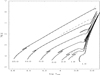 |
Fig. 1. HR diagram for some selected models. The masses are indicated in solar units. Continuous lines represent the present models while dashed ones denote the models by Claret (2004). Solar composition. |
Concerning the theoretical apsidal motion constants, in general, the new models are more concentrated in mass than the old ones (Fig. 2). However, the differences are not constant and progressively decrease from less massive to more massive models. Considering, for example, models of 1.00 M⊙, the difference is of the order of 0.20 dex (in the logarithmic scale) in the middle of the main sequence, which is of the order of the mean observational errors. For the more massive models (e.g. 2.50 and 5.00 M⊙), the differences between the new models and the old models are only of the order of 0.05 dex, though they are still important.
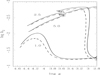 |
Fig. 2. Apsidal motion constant of order two for new and old models. The masses, in solar units, are indicated by numbers. Same captions as in Fig. 1. |
The differences between the two sets of models discussed above have diverse causes, such as the adopted values of αMLT (1.84 and 1.68). The equation of state also contributes. It is important to note that this is mainly the case for the less massive models. The rates of mass loss, which are different from those adopted in the 2004 models, also influence both the shape of the tracks in the HR diagram and their internal structure. Another reason for the differences in the 2004 models is that a constant value for the amount of core overshooting was adopted for all masses; conversely, as previously mentioned, we introduced a dependence on the stellar mass for the core overshooting as given by Claret & Torres (2018).
The effects of the metallicity on the internal structure is shown in Fig. 3 for models with 1.00 and 5.00 M⊙ for [Fe/H = 0.00] with continuous lines, and for [Fe/H = −1.00] with dashed lines. The differences between the [Fe/H = 0.00] and [Fe/H = −1.00] models are important. This mainly concerns less massive models during the main sequence and can achieve up to 0.80 dex for the 1.00 M⊙ models. These differences, in general, decrease with the stellar mass.
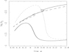 |
Fig. 3. Apsidal motion constant of order two for present models. Computed for [Fe/H] = 0.00 (continuous lines) and for [Fe/H] = −1.0 (dashed lines). Models with 1.00 and 5.00 M⊙. |
For homogeneous models, the radius of gyration shows a different behaviour for masses larger or smaller than ≈1.5 M⊙, that is there is a minimum of β around this value. Such behaviour is connected with the change in the dominant source of thermonuclear energy from the pp chain to the CNO cycle (Fig. 2 by Claret & Giménez 1989). In Fig. 4, we show the evolution of β for models of 1.00, 2.50, and 5.00 M⊙. When the star evolves, the behaviour of β becomes more complex, showing some loops for advanced evolutionary phases. Despite the complex behaviour of the apsidal motion constant of order two and the radius of gyration as a function of log g shown in Figs. 2 and 4, both have an approximately linear relationship that is independent of their evolution for a wide range of stellar masses. The resulting lobe shown in Fig. 5 is due to nuclear reactions and chemical inhomogeneities which lead to structural changes. The aspect of Fig. 5 is not surprising given that log k2 and log β give a measure of the mass concentration for each evolutionary stage of the models through the integration of the respective differential equations of second and first order, respectively.
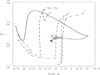 |
Fig. 4. The evolution of radius of gyration for some selected models. Continuous line represents the model with 1.00 M⊙, the dashed and dashed-point lines denote the models with 2.5 and 5.0 M⊙, respectively. Solar composition. |
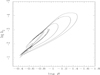 |
Fig. 5. Relationship between evolving log β and log k2 for models with 1.00, 2.50, 5.00, 10.00, 15.00, 20.00, and 25.00 M⊙. Solar composition. |
Finally, Table 1 summarises the data available at the CDS or directly from the author. Additional calculations for other chemical compositions and/or for specific masses can be performed upon request.
Acknowledgments
I am grateful to the anonymous referee for the careful reading of the paper and for her/his helpful suggestions. I am grateful to B. Rufino, G. Torres, and V. Costa for their useful comments. The Spanish MEC (AYA2015-71718-R and ESP2017-87676-C5-2-R) is gratefully acknowledged for its support during the development of this work. AC also acknowledges financial support from the State Agency for Research of the Spanish MCIU through the Center of Excellence Severo Ochoa award for the Instituto de Astrofísica de Andalucía (SEV-2017-0709). This research has made use of the SIMBAD database, operated at the CDS, Strasbourg, France, and of NASA’s Astrophysics Data System Abstract Service.
References
- Albrecht, S., Reffert, S., Snellen, I. A. G., & Winn, J. N. 2009, Nature, 461, 373 [NASA ADS] [CrossRef] [PubMed] [Google Scholar]
- Asplund, M., Grevesse, N., Sauval, A. J., & Scott, P. 2009, ARA&A, 47, 481 [NASA ADS] [CrossRef] [Google Scholar]
- Blocker, T. 1995, A&A, 297, 727 [Google Scholar]
- Claret, A. 1997, A&A, 327, 11 [NASA ADS] [Google Scholar]
- Claret, A. 1999, A&A, 350, 56 [NASA ADS] [Google Scholar]
- Claret, A. 2004, A&A, 424, 919 [NASA ADS] [CrossRef] [EDP Sciences] [Google Scholar]
- Claret, A. 2012, A&A, 543, A67 [NASA ADS] [CrossRef] [EDP Sciences] [Google Scholar]
- Claret, A. 2014, A&A, 562, A31 [NASA ADS] [CrossRef] [EDP Sciences] [Google Scholar]
- Claret, A., & Hempel, M. 2013, A&A, 552, A29 [NASA ADS] [CrossRef] [EDP Sciences] [Google Scholar]
- Claret, A., & Giménez, A. 1989, A&AS, 81, 37 [NASA ADS] [Google Scholar]
- Claret, A., & Giménez, A. 1991, A&A, 244, 319 [NASA ADS] [Google Scholar]
- Claret, A., & Giménez, A. 1993, A&A, 277, 487 [Google Scholar]
- Claret, A., & Giménez, A. 2010, A&A, 519, A57 [NASA ADS] [CrossRef] [EDP Sciences] [Google Scholar]
- Claret, A., & Torres, G. 2018, ApJ, 859, 100 [NASA ADS] [CrossRef] [Google Scholar]
- Claret, A., & Willems, B. 2002, A&A, 388, 518 [NASA ADS] [CrossRef] [EDP Sciences] [Google Scholar]
- Claret, A., Torres, G., & Wolf, M. 2010, A&A, 515, A4 [NASA ADS] [CrossRef] [EDP Sciences] [Google Scholar]
- Collins, II., G. W. 2003, The Virial Theorem in Stellar Astrophysics, Web Edition [Google Scholar]
- Freytag, B., Ludwig, H.-G., & Steffen, M. 1996, A&A, 313, 497 [Google Scholar]
- Grevesse, N., & Sauval, A. J. 1998, Space Sci. Rev., 85, 161 [NASA ADS] [CrossRef] [Google Scholar]
- Herwig, F., Bloecker, T., Schoenberner, D., & El Eid, M. 1997, A&A, 324, L81 [NASA ADS] [Google Scholar]
- Hut, P. 1981, A&A, 99, 126 [NASA ADS] [Google Scholar]
- Hut, P. 1982, A&A, 102, 37 [NASA ADS] [Google Scholar]
- Kopal, Z. 1959, Close Binary Systems (London: Chapman and Hall) [Google Scholar]
- Kopal, Z. 1978, Dynamics of Close Binary Systems (Dordrecht, Holland: Reidel) [CrossRef] [Google Scholar]
- Magic, Z., Weiss, A., & Asplund, M. 2015, A&A, 573, A89 [NASA ADS] [CrossRef] [EDP Sciences] [Google Scholar]
- Paxton, B., Bildsten, L., Dotter, A., et al. 2011, ApJS, 192, 3 [Google Scholar]
- Paxton, B., Cantiello, M., Arras, P., et al. 2013, ApJS, 208, 4 [NASA ADS] [CrossRef] [Google Scholar]
- Paxton, B., Marchant, P., Schwab, J., et al. 2015, ApJS, 220, 15 [Google Scholar]
- Reimers, D. 1977, A&A, 61, 217 [NASA ADS] [Google Scholar]
- Torres, G., Andersen, J., & Giménez, A. 2010, A&ARv, 18, 67 [Google Scholar]
- Vink, J. S., de Koter, A., & Lamers, H. J. G. L. M. 2001, A&A, 369, 574 [NASA ADS] [CrossRef] [EDP Sciences] [Google Scholar]
- Willems, B., & Claret, A. 2003, A&A, 410, 289 [NASA ADS] [CrossRef] [EDP Sciences] [Google Scholar]
- Zasche, P., & Wolf, M. 2019, AJ, 157, 87 [NASA ADS] [CrossRef] [Google Scholar]
All Tables
All Figures
|
Fig. 1. HR diagram for some selected models. The masses are indicated in solar units. Continuous lines represent the present models while dashed ones denote the models by Claret (2004). Solar composition. |
| In the text | |
|
Fig. 2. Apsidal motion constant of order two for new and old models. The masses, in solar units, are indicated by numbers. Same captions as in Fig. 1. |
| In the text | |
|
Fig. 3. Apsidal motion constant of order two for present models. Computed for [Fe/H] = 0.00 (continuous lines) and for [Fe/H] = −1.0 (dashed lines). Models with 1.00 and 5.00 M⊙. |
| In the text | |
|
Fig. 4. The evolution of radius of gyration for some selected models. Continuous line represents the model with 1.00 M⊙, the dashed and dashed-point lines denote the models with 2.5 and 5.0 M⊙, respectively. Solar composition. |
| In the text | |
|
Fig. 5. Relationship between evolving log β and log k2 for models with 1.00, 2.50, 5.00, 10.00, 15.00, 20.00, and 25.00 M⊙. Solar composition. |
| In the text | |
Current usage metrics show cumulative count of Article Views (full-text article views including HTML views, PDF and ePub downloads, according to the available data) and Abstracts Views on Vision4Press platform.
Data correspond to usage on the plateform after 2015. The current usage metrics is available 48-96 hours after online publication and is updated daily on week days.
Initial download of the metrics may take a while.