| Issue |
A&A
Volume 674, June 2023
|
|
|---|---|---|
| Article Number | A67 | |
| Number of page(s) | 7 | |
| Section | Catalogs and data | |
| DOI | https://doi.org/10.1051/0004-6361/202346250 | |
| Published online | 01 June 2023 | |
Theoretical tidal evolution constants for stellar models from the pre-main sequence to the white dwarf stage
Apsidal motion constants, moment of inertia, and gravitational potential energy★
1
Instituto de Astrofísica de Andalucía, CSIC,
Apartado 3004,
18080
Granada,
Spain
e-mail: This email address is being protected from spambots. You need JavaScript enabled to view it.
2
Dept. Física Teórica y del Cosmos, Universidad de Granada,
Campus de Fuentenueva s/n,
10871
Granada,
Spain
Received:
26
February
2023
Accepted:
2
April
2023
Abstract
Aims. One of the most reliable means of studying the stellar interior is through the apsidal motion in double line eclipsing binary systems since these systems present errors in masses, radii, and effective temperatures of only a few per cent. On the other hand, the theoretical values of the apsidal motion to be compared with the observed values depend on the stellar masses of the components and more strongly on their radii (fifth power). The main objective of this work is to make available grids of evolutionary stellar models that, in addition to the traditional parameters (e.g. age, mass, log g, Teff), also contain the necessary parameters for the theoretical study of apsidal motion and tidal evolution. This information is useful for the study of the apsidal motion in eclipsing binaries and their tidal evolution, and can also be used for the same purpose in exoplanetary systems.
Methods. All models were computed using the MESA package. We consider core overshooting for models with masses ≥1.2M⊙. For the amount of core overshooting we adopted a recent relationship for mass × core overshooting. We adopted for the mixing-length parameter αMLT the value 1.84 (the solar-calibrated value). Mass loss was taken into account in two evolutionary phases. The models were followed from the pre-main sequence phase to the white dwarf (WD) stage.
Results. The evolutionary models containing age, luminosity, log g, and Teff, as well as the first three harmonics of the internal stellar structure (k2, k3, and k4), the radius of gyration βy, and the dimensionless variable α, related to gravitational potential energy, are presented in 69 tables covering three chemical compositions: [Fe/H] = −0.50, 0.00, and 0.50. Additional models with different input physics are available.
Key words: binaries: close / binaries: eclipsing / stars: evolution / stars: interiors
Tables 1–69 are only available at the CDS via anonymous ftp to cdsarc.cds.unistra.fr (130.79.128.5) or via https://cdsarc.cds.unistra.fr/viz-bin/cat/J/A+A/674/A67
© The Authors 2023
 Open Access article, published by EDP Sciences, under the terms of the Creative Commons Attribution License (https://creativecommons.org/licenses/by/4.0), which permits unrestricted use, distribution, and reproduction in any medium, provided the original work is properly cited.
This article is published in open access under the Subscribe to Open model. This email address is being protected from spambots. You need JavaScript enabled to view it. to support open access publication.
1 Introduction
Double line eclipsing binary systems (DLEBS) are the best sources for obtaining absolute stellar parameters with great precision. In addition, because of their proximity, some effects may appear due to the interaction of the two components, such as mutual irradiation, tidal distortion, and mass exchange. DLEBS are very important in astrophysics because the perturbations due to the proximity of the two components act as probes and make it possible to investigate in detail the evolution and in some particular cases their internal structure. In this sense, such perturbations play a very similar role to that of the usual techniques of physics labs in which objects are perturbed applying for example a magnetic and/or electric field and studying its behaviour under the action of the applied perturbations.
In the case of DLEBS the presence of the companion changes the gravitational field of both, which affects the equilibrium configuration of both components (effect of tides). This alteration is responsible for the loss of spherical symmetry of the binary components and it depends on the internal structure of the components. The two stars can also be distorted by the effect of the rotation that tends to flatten them on the poles. From the theoretical point of view, it is possible to describe such distortions as a function of the internal structure of both stars. The orbit of this pair of stars will not be Keplerian because the orbital elements will be functions of time, in particular the argument of periastron ω. In general, there are three physical phenomena that can give rise to apsidal motion: the loss of the spherical symmetry by distortions; the presence of a third body; and a relativistic effect, the best known example being the advance of perihelion of the planet Mercury.
On the other hand, earlier comparisons between the internal structure constants derived from the observed apsidal motions were reported a long time ago; they indicate that stellar structure is more centrally concentrated in mass than those extracted from the stellar evolutionary models (see e.g. Introduction in Claret & Giménez 1993). Such discrepancies were partially resolved later by (Claret & Giménez 1993, 2010) considering new times of minima, new opacity tables, and core overshooting.
For several years the apsidal motion of DI Her was a serious problem since the comparison between the theoretical calculations and the observed value of  differed by almost 500%. Various mechanisms were invoked to explain such a discrepancy, including alternative theories of gravitation. For the confrontation of theory and observational data, Claret (1998) analysed some aspects of the apsidal motion of DI Her. The main conclusion of that paper was that an alternative theory of gravitation was not necessary to explain the observational value of the apsidal motion. Finally the case of DI Her was solved observationally through the Rossiter-McLaughlin effect by Albrecht et al. (2009). Later Claret et al. (2010) using the data obtained by Albrecht et al. (2009), mainly those related to the Rossiter-McLaughlin effect, found a good agreement between the theoretical value of k2 and its observational counterpart. More recently, Liang et al. (2022), using TESS data combined with previous observations, obtained a significant result since the three-dimensional spin directions of the two components of DI Her could be determined. With these data these authors have found good agreement between k2theo, provided by Claret et al. (2021), and its observational counterpart.
To the best of our knowledge, the last systematic comparison between theoretical and observed values of apsidal motion rates was carried out by Claret et al. (2021) who used an observational sample of 27 selected DLEBS to compare the theoretical values of k2 with their observational counterparts. These authors have used minimum times extracted from the light curves provided by the Transiting Exoplanet Survey Satellite (TESS). Very good agreement has been found between the theoretically predicted values and their observational counterparts, including the troublesome case of DI Her.
Another very important contribution to the study of apsidal motion came from a group from the Astronomical Institute at Charles University. Zasche & Wolf (2019) investigated 21 eccentric eclipsing binaries (early-type) located in the Small Magellanic Cloud and determined their apsidal motions and analysed their respective light curves. More recently Zasche et al. (2021) present an extensive sample of 162 early-type binary systems showing apsidal motion located in the Large Magellanic Cloud. This point is particularly important given that light curves and apsidal motion modelling were carried out for the first time for several systems simultaneously and in an environment with a chemical composition different from solar (for a more recent reference on apsidal motion measurements, see Zasche et al. 2023).
The comments in the previous paragraphs refer mainly to DLEBS that are still on the main sequence or close to it. Burdge et al. (2019) studied the orbital decay of compact stars in a hydrogen-poor low-mass white dwarf (WD), FJ053332.05+020911.6. One of the components of this system exhibits ellipsoidal variations due to tidal distortions. The estimated mass for this component (PTF J0533+0209B) is of the order of 0.20 M⊙. We note that the gravity-darkening effect must also be taken into account for compact stars distorted by tides and/or rotation (Claret 2021). Until then we computed our evolutionary stellar models containing internal structure constants only up to the giant phases. For the case of PTFJ053332.05+020911.6 and other similar systems, where at least one WD has been detected, we decided to extend our grids from the pre-main sequence (PMS) to the WD phase. This is the main objective of the present paper.
2 Stellar evolutionary models: Apsidal motion internal constants, momentum of inertia, and gravitational potential energy
The evolutionary tracks were computed using the Modules for Experiments in Stellar Astrophysics package (MESA; see Paxton et al. 2011, 2013, 2015; v7385). We introduced a subroutine to compute the apsidal motion constants (k2, k3, k4), the moment of inertia, and the gravitational potential energy. In this paper we do not consider directly the effects of rotation. The adopted mixing-length parameter αMLT was 1.84 (the solar-calibrated value; Torres et al. 2015). However, the αMLT parameter seems to depend on the evolutionary status and/or metallicity, as shown by Magic et al. (2015) using 3D simulations. As commented in Claret (2019), it is not easy to compare these results with those coming from MESA, due to the different input physics, for example the equation of state and opacities. For the opacities we adopted the element mixture given by Asplund et al. (2009). The helium content follows the enrichment law Y = Yp + 1.67Z, where Yp is the primordial helium content (Ade et al. 2016).
The mass range covers the interval from 0.2 to 8.0 M⊙ for three chemical compositions: [Fe/H] −0.5, 0.00, and +0.50. The grids for the two extra chemical compositions, [Fe/H ] = −0.50 and 0.50, were computed to take into account observational errors in [Fe/H] for systems located in the solar environment.
As commented in the Introduction, the evolutionary tracks were computed from the PMS up to the WD stage. We adopted the following scheme for mass loss: for the interval 0.2−1.8 M⊙ we followed the recipe by Reimers (1977) with ηR = 0.1 and for the AGB scheme we adopted the formalism by Blocker (1995) with ηB = 10.0. For models more massive than 1.8 M⊙ we assumed ηR = 0.1 and ηB = 30.0. The adopted wind switch RGB-AGB was 1.0×10⁻⁴.
Convective core overshooting was considered for models with stellar mass higher than or equal to 1.2 M⊙. In this paper we adopt the diffusive approximation, represented by the free parameter fov (Freytag et al. 1996; Herwig et al. 1997). The diffusion coefficient in the overshooting region is given by the expression  , where Do is the diffusion coefficient at the convective boundary, z is the geometric distance from the edge of the convective zone, Hv is the velocity scale-height at the convective boundary expressed as Hv = fov Hp, and the coefficient fov is a free parameter that governs the width of the overshooting layer. It is known that models computed adopting core overshooting are more centrally concentrated in mass than their standard counterparts following Claret & Giménez (1991). For the amount of core overshooting we adopted the relationship between the stellar mass and fov derived by Claret & Torres (2019), instead of adopting a single value of core overshooting for the entire range of masses, as was done in the past.
2.1 Apsidal motion constants: k2, k3, and k4
The theoretical apsidal motion constants k2, k3, and k4 were derived simultaneously by integrating the Radau equation using a fifth-order Runge-Kutta method, with a tolerance level of 10−7 :
 (1)
(1)
Here the auxiliary parameter ηj is given by
 (2)
(2)
In Eq. (1), a denotes the mean radius of the stellar configuration, ϵj; is a measure of the deviation from sphericity, ρ(a) is the mass density at the distance a from the centre of the configuration, and  is the mean mass density within a sphere of radius a.
The apsidal motion constant of order j is given by
 (3)
(3)
where ηj(R) indicates the values of ηj at the surface of the star. We note that these equations were derived in the framework of static tides. For the case of dynamic tides, we need to treat with more elaborated equations because the rate of static tides is derived assuming that the orbital period is larger than the periods of the free oscillation modes. However, dynamic tides can significantly change this scenario due to the effects of the compressibility of the stellar fluid. This is important in systems that are nearly synchronized. In this case, for higher rotational angular velocities, additional deviations due to resonances appear if the forcing frequencies of the dynamic tides come into the range of the free oscillation modes of the component stars. The role of dynamical tides was evaluated for some DLEBS by Claret & Willems (2002), Willems & Claret (2003), Claret & Giménez (2010), and more recently in Claret et al. (2021).
As mentioned in the Introduction, our stellar evolutionary tracks were computed without taking rotation into account. In order to evaluate the effects of rotation on the apsidal motion constants, a correction on the internal structure constants was proposed by Claret (1999). This correction is given by the equation
 (4)
(4)
Here λ = 2V2/(3gR), where g is the surface gravity and V is the equatorial rotational velocity.
Figure 1 shows the Hertzprung–Russell diagram (HR) for some selected models: 0.70, 1.00, 1.40, 3.00, and 8.00 M⊙. In Figs. 2 and 3 we show the evolution of log k2 as a function of log g for models with initial masses of 8.00 and 1.00 M⊙, respectively. The behaviour of the two models is similar when they reach the WD stage (log k2 is of the order of −1.00). This implies that, using simple models based on polytropes, the equivalent n would be of the order of 2.1, where n is the polytropic index. This data confirm the earlier calculations for WD using polytropes as input physics. We recall that for the case of non-relativistic electrons n ≈ 1.5 and for the case of relativistic electrons n = 3.0 this index would be ≈2.0 (see Kopal 1959, p. 35).
The parameter k2 is applied in the studies of apsidal motion of DLEBS and/or exoplanets, and is also useful for computing tidal evolution. For example, the differential equations that govern the tidal evolution depend not only on this parameter, but also on the radius of gyration (see Hut 1981, 1982). We can write the corresponding differential equations as
 (5)
(5)
 (6)
(6)
 (7)
(7)
 (8)
(8)
In the above equations e represents the orbital eccentricity, A is the semi-major axis, Mi; is the mass of component i, Ωi is the angular velocity of the component i, ω is the mean orbital angular velocity, Ri is the radius of the component i, q = M2/M1, q2=M1/M2, and tFi is an estimation of the timescale of tidal friction for each component.
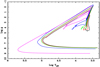 |
Fig. 1 Hertzprung-Russell diagram for some models from the PMS to cooling WD stage. The masses of the models are (from right to left) 0.7 (black), 1.0 (red), 1.4 (green), 3.0 (blue), and 8.0 (magenta) in solar units. αMLT = 1.84, [Fe/H] = 0.00. |
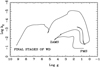 |
Fig. 2 Behaviour of logk2 as a function of log g. [Fe/H]=0.00, initial mass of 8.00 M⊙. |
2.2 Calculation of gravitational potential energy Ω and moment of inertia I
As indicated by Claret (2019) the effects of General Relativity on the calculation of the moment of inertia and gravitational potential energy can be neglected for stars during the PMS, main sequence, and even for WD. However, for consistency with our previous papers on compact stars, here we adopt the relativistic formalism throughout. Therefore, the moment of inertia can be computed using the equations
![Mathematical equation: $ \matrix{ {J = {{8\pi } \over 3}\int_0^R {{\rm{\Lambda }}\left( r \right){r^4}\left[ {\rho \prime \left( r \right) + P{{\left( r \right)} \mathord{\left/ {\vphantom {{\left( r \right)} {{c^2}}}} \right. \kern-\nulldelimiterspace} {{c^2}}}} \right]{\rm{d}}r,} } \hfill \cr {I \approx {J \over {\left( {1 + {{2GJ} \over {{R^3}{c^2}}}} \right)}} \equiv {{\left( {\beta R} \right)}^2}M,} \hfill \cr } $](/articles/aa/full_html/2023/06/aa46250-23/aa46250-23-eq12.png) (9)
(9)
where β is the radius of gyration.
The gravitational energy of a spherically symmetric star can be written as
![Mathematical equation: $ {\rm{\Omega = }} - 4\pi \,\int_0^R {{r^2}\rho \prime \left( r \right)\,\left[ {{{\rm{\Lambda }}^{{1 \mathord{\left/ {\vphantom {1 2}} \right. \kern-\nulldelimiterspace} 2}}}\left( r \right) - 1} \right]} \,{\rm{d}}r \equiv - \alpha {{G{M^2}} \over R}. $](/articles/aa/full_html/2023/06/aa46250-23/aa46250-23-eq13.png) (10)
(10)
In the above equation P(r) is the pressure, ρ′(r) the energy density, and the function Λ(r) is given by ![Mathematical equation: ${\left[ {1 - {{2Gm\left( r \right)} \over {r{c^2}}}} \right]^{ - 1}}$](/articles/aa/full_html/2023/06/aa46250-23/aa46250-23-eq14.png) . The parameter α is a dimensionless number that measures the relative mass concentration. In the case of less elaborated stellar models (e.g. polytropes), we have α = 3/(5 − n), where n is the polytropic index. Equations (9) and (10) were integrated simultaneously adopting the same numerical scheme and tolerance level as in Eq. (1).
. The parameter α is a dimensionless number that measures the relative mass concentration. In the case of less elaborated stellar models (e.g. polytropes), we have α = 3/(5 − n), where n is the polytropic index. Equations (9) and (10) were integrated simultaneously adopting the same numerical scheme and tolerance level as in Eq. (1).
2.3 Some interesting properties of the moment of inertia and the gravitational potential energy: The Γ function
The factors α or and β are connected through the function Γ introduced by Claret (2012) and improved by Claret & Hempel (2013), which is defined as
![Mathematical equation: $ {\rm{\Gamma }}\left( {{\rm{mass,}}\,{\rm{EOS}}} \right) \equiv {{\left[ {\alpha \beta } \right]} \over {{\rm{\Lambda }}{{\left( R \right)}^{0.8}}}}, $](/articles/aa/full_html/2023/06/aa46250-23/aa46250-23-eq15.png) (11)
(11)
where EOS is the equation of state.
One of the most striking properties of this function is that the final products of stellar evolution (white dwarfs, neutron-quark hybrids, and proto-neutron stars at the onset of formation of black holes) recover the value calculated for the PMS stage (i.e. Γ(mass, EOS)) ≈ 0.40. We note for the last four mentioned systems that the effects of General Relativity are strong. This invariance was also extended to models of gaseous planets with masses between 0.1 and 50.0 MJupiter, following from the gravitational contraction up to an age of ≈20 Myr. As a consequence of this invariance a macroscopic stability criterion for neutron, hybrid, and quark star models was established. More detailed information on this function, the ‘memory effect’, and the stability criterion can be found in Claret (2012, 2014), Claret & Hempel (2013).
As examples of the behaviour of Γ(mass, EOS), Figs. 4 and 5 show the invariance of such a function for the PMS-WD stages for two different models, 7.00 and 0.40 M⊙, respectively, adopting the solar composition. In both figures Γ(mass, EOS) increases by about three orders of magnitude with respect to its value at PMS (this increase is not shown fully in Figs. 4 and 5 due to the chosen scale).
On the other hand, it is clear from both figures that there is a connection between the values of Γ(mass, EOS) and the total thermal power from PP, CNO, and triple-α: the larger the thermonuclear contributions, the larger the value of Γ(mass, EOS). During the PMS phase, when the chemical composition is homogeneous, Γ(mass, EOS) ≈ 0.40 and ϵN ≈ 0.0. However, in the WD phase, although the initial chemical composition has been altered by thermonuclear reactions, the value 0.40 is recovered, given that these reactions cease. In summary, the property of Γ(mass, EOS) presents the same value (≈0.40) in the initial and final stages of stellar evolution. We confirmed this behaviour for all the models of our grids. This behaviour is also valid for gaseous planets, neutron-quark-hybrid stars, and proto-neutron stars at the onset of formation of black holes.
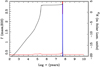 |
Fig. 4 Time evolution of the function Γ(mass, EOS) for a model with initial mass of 7.00 M⊙ evolving from the PMS to the WD stage, αMLT=1.84, fov = 0.016, [Fe/H]=0.00. The red line represents Γ(mass, EOS), while the black line indicates the total thermal power from PP and CNO (excluding neutrinos) and the blue line indicates the total thermal power from triple-α (also excluding neutrinos). The nuclear power ϵN is in logarithmic scale. |
3 Final remarks and table organization
We computed three evolutionary grids covering three metallicities: [Fe/H) = −0.50, 0.00, and +0.50 from PMS to the WD stage. The covered mass range was 0.20−8.00 M⊙. For such models, in addition to the characteristic parameters (age, luminosity, log g, effective temperatures), the internal structure constants (k2, k3, k4), the moment of inertia, and the gravitational potential energy have also been computed. The resulting tables have been prepared mainly for studies of DLEBS and/or exoplanetary systems. Tables I–III summarize the input physics for each series of models, while Tables 1–69 contain the necessary theoretical inputs for the comparison with the absolute dimensions of the DLEBS as well as the necessary parameters for the apsidal motion and tidal evolution studies.
Acknowledgements
I thank M. Broz for his pertinent comments and suggestions that have improved this paper. The Spanish MEC (AYA2015-71718-R and ESP2017-87676-C5-2-R) is gratefully acknowledged for its support during the development of this work. AC also acknowledges financial support from the grant CEX2021-001131-S funded by MCIN/AEI/10.13039/501100011033. This research has made use of the SIMBAD database, operated at the CDS, Strasbourg, France, and of NASA’s Astrophysics Data System Abstract Service.
Appendix A Brief description of Tables A1, A2, and A3
Tables A1, A2, and A3 summarize the type of data available (for more details, see the ReadMe file on the CDS).
Mass and initial chemical composition
Mass and initial chemical composition
Mass and initial chemical composition
References
- Ade, P. A. R., Aghanim, N., Arnaud, M., et al. 2016, A&A, 594, A13 [NASA ADS] [CrossRef] [EDP Sciences] [Google Scholar]
- Albrecht, S., Reffert, S., Snellen, I. A. G., & Winn, J. N. 2009, Nature, 461, 373 [Google Scholar]
- Asplund, M., Grevesse, N., Sauval, A. J., & Scott, P. 2009, ARA&A, 47, 481 [NASA ADS] [CrossRef] [Google Scholar]
- Blocker, T. 1995, A&A, 297, 727 [Google Scholar]
- Burdge, K. B., Fuller, J., Phinney, E. S. et al. 2019, ApJ, 886 L12 [NASA ADS] [CrossRef] [Google Scholar]
- Claret, A. 1998 A&A, 330, 533 [NASA ADS] [Google Scholar]
- Claret, A. 1999, A&A, 350, 56 [NASA ADS] [Google Scholar]
- Claret, A. 2004, A&A, 424, 919 [NASA ADS] [CrossRef] [EDP Sciences] [Google Scholar]
- Claret, A. 2012, A&A, 543, A67 [NASA ADS] [CrossRef] [EDP Sciences] [Google Scholar]
- Claret, A. 2014, A&A, 562A, 31 [Google Scholar]
- Claret, A. 2019, A&A, 628A, 29 [Google Scholar]
- Claret, A. 2021, A&A, 648A, 111 [Google Scholar]
- Claret, A., & Giménez, A. 1991, A&A, 244, 319 [NASA ADS] [Google Scholar]
- Claret, A., & Giménez, A. 1993, A&A, 277, 487 [Google Scholar]
- Claret, A., & Giménez, A. 2010, A&A, 519A, 57 [Google Scholar]
- Claret, A., & Hempel, M. 2013, A&A, 552A, 29 [Google Scholar]
- Claret, A., & Torres, G. 2019, ApJ, 876, 134 [Google Scholar]
- Claret, A., & Willems, B. 2002, A&A, 388, 518 [NASA ADS] [CrossRef] [EDP Sciences] [Google Scholar]
- Claret, A., Torres, G., & Wolf, M. 2010, A&A, 515, A4 [NASA ADS] [CrossRef] [EDP Sciences] [Google Scholar]
- Claret, A., Giménez, A., Baroch, D., et al. 2021, A&A, 654, A17 [NASA ADS] [CrossRef] [EDP Sciences] [Google Scholar]
- Freytag, B., Ludwig, H.-G., Steffen, M. 1996, A&A, 313, 497 [NASA ADS] [Google Scholar]
- Herwig, F., Bloecker, T., Schoenberner, D., & El Eid, M. 1997, A&A, 324, L81 [NASA ADS] [Google Scholar]
- Hut, P. 1981, A&A, 99, 126 [NASA ADS] [Google Scholar]
- Hut, P. 1982, A&A, 102, 37 [NASA ADS] [Google Scholar]
- Kopal, Z. 1959, Close Binary Systems (London: Chapman and Hall) [Google Scholar]
- Liang, Y., Winn, J. N., & Albrecht, S. H. 2022, ApJ, 927, 114 [NASA ADS] [CrossRef] [Google Scholar]
- Magic, Z., Weiss, A., & Asplund, M. 2015, A&A, 573, A89 [NASA ADS] [CrossRef] [EDP Sciences] [Google Scholar]
- Paxton, B., Bildsten, L., Dotter, A., et al. 2011, ApJS, 192, 3 [Google Scholar]
- Paxton, B., Cantiello, M., Arras, P., et al. 2013, ApJS, 208, 4 [Google Scholar]
- Paxton, B., Marchant, P., Schwab, J., et al. 2015, ApJS, 220, 15 [Google Scholar]
- Reimers, D. 1977, A&A, 61, 217 [NASA ADS] [Google Scholar]
- Torres, G., Claret, A., Pavlovski, K., & Dotter, A. 2015, ApJ, 807, 26 [NASA ADS] [CrossRef] [Google Scholar]
- Willems, B., & Claret, A. 2003, A&A, 410, 289 [NASA ADS] [CrossRef] [EDP Sciences] [Google Scholar]
- Zasche, P., & Wolf, M. 2019, AJ, 157, 87 [Google Scholar]
- Zasche, P., Wolf, M., Kučáková, H., et al. 2020, A&A, 640, A33 [NASA ADS] [CrossRef] [EDP Sciences] [Google Scholar]
- Zasche, P., Borkovits, P., Jayaraman, R., et al. 2023, MNRAS, 520, 3127 [NASA ADS] [CrossRef] [Google Scholar]
All Tables
All Figures
|
Fig. 1 Hertzprung-Russell diagram for some models from the PMS to cooling WD stage. The masses of the models are (from right to left) 0.7 (black), 1.0 (red), 1.4 (green), 3.0 (blue), and 8.0 (magenta) in solar units. αMLT = 1.84, [Fe/H] = 0.00. |
| In the text | |
|
Fig. 2 Behaviour of logk2 as a function of log g. [Fe/H]=0.00, initial mass of 8.00 M⊙. |
| In the text | |
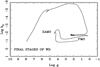 |
Fig. 3 Same as Fig. 2, but for an initial mass of 1.00 M⊙. |
| In the text | |
|
Fig. 4 Time evolution of the function Γ(mass, EOS) for a model with initial mass of 7.00 M⊙ evolving from the PMS to the WD stage, αMLT=1.84, fov = 0.016, [Fe/H]=0.00. The red line represents Γ(mass, EOS), while the black line indicates the total thermal power from PP and CNO (excluding neutrinos) and the blue line indicates the total thermal power from triple-α (also excluding neutrinos). The nuclear power ϵN is in logarithmic scale. |
| In the text | |
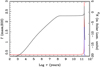 |
Fig. 5 Same as Fig. 4, but for a model with initial mass of 0.40 M⊙ and fov = 0.000. |
| In the text | |
Current usage metrics show cumulative count of Article Views (full-text article views including HTML views, PDF and ePub downloads, according to the available data) and Abstracts Views on Vision4Press platform.
Data correspond to usage on the plateform after 2015. The current usage metrics is available 48-96 hours after online publication and is updated daily on week days.
Initial download of the metrics may take a while.