| Issue |
A&A
Volume 675, July 2023
|
|
|---|---|---|
| Article Number | A135 | |
| Number of page(s) | 7 | |
| Section | Catalogs and data | |
| DOI | https://doi.org/10.1051/0004-6361/202245181 | |
| Published online | 11 July 2023 | |
Centaurus X-3 orbital ephemerides using Insight-HXMT, RXTE, Swift/BAT, and NuSTAR observations
1
Institut für Astronomie und Astrophysik,
Sand 1,
72076
Tübingen,
Germany
e-mail: This email address is being protected from spambots. You need JavaScript enabled to view it.
2
School of Physics and Astronomy, Sun Yat-Sen University,
Zhuhai
519082,
PR China
3
Key Laboratory for Particle Astrophysics, Institute of High Energy Physics, Chinese Academy of Sciences,
19B Yuquan Road,
Beijing
100049,
PR China
4
University of Chinese Academy of Sciences, Chinese Academy of Sciences,
Beijing
100049,
PR China
Received:
11
October
2022
Accepted:
4
April
2023
Abstract
Centaurus X-3 (Cen X-3) is the first X-ray pulsar discovered and has been studied for decades by multiple facilities, allowing for accurate measurements of the decay rate of the orbital period of the binary system. However, the most recent study of the orbital parameters of the system dates back to the RXTE era. For this study, we have complemented these measurements with the more recent high-quality Insight-HXMT and NuSTAR data obtained 20 yr later to improve constraints on the orbital period decay rate and eccentricity of the system through pulsar timing analysis. In addition, we also used long-term monitoring by Swift/BAT to independently measure orbital period evolution through eclipse timing. As a result, improved orbital ephemerides including accurate estimates of the orbital period, the period decay rate, and eccentricity of the system were obtained.
Key words: binaries: eclipsing / pulsars: individual: Cen X-3 / X-rays: binaries
© The Authors 2023
 Open Access article, published by EDP Sciences, under the terms of the Creative Commons Attribution License (https://creativecommons.org/licenses/by/4.0), which permits unrestricted use, distribution, and reproduction in any medium, provided the original work is properly cited.
This article is published in open access under the Subscribe to Open model. This email address is being protected from spambots. You need JavaScript enabled to view it. to support open access publication.
1 Introduction
Evolution of orbital separation and eccentricity in high mass X-ray binaries (HMXBs) is driven by several not yet fully understood mechanisms, which are particularly interesting in the context of the emerging gravitational wave astronomy (i.e. observations of merging black hole and neutron star systems). One of the most interesting objects in this regard is Centaurus X-3 (Cen X-3), the first X-ray pulsar ever discovered in 1967 during the testing of rocket-borne proportional counters (Chodil et al. 1967) and extensively studied ever since. Analysis of observations with UHURU (Giacconi et al. 1971) allowed for the detection of pulsations with a period of ~4.8 s, and a modulation of the pulsed frequency associated with motion in a binary system with an orbital period of Porb ~2.1 days (Schreier et al. 1972). The latter conclusion was confirmed by the discovery of regular X-ray eclipses lasting for approximately one-fourth of the orbital phase and observed each orbital cycle. The optical companion, named Krzeminski’s Star, was discovered in 1974 by Krzeminski (1974). Currently it is understood that the binary system consists of a neutron star with a mass of MN = 1.21(21) M⊙ and a type O(6–7) II–III companion with a mass of MC = 20.5(7) M⊙ (Ash et al. 1999), and it is therefore classified as a HMXB.
Already the first UHURU observations suggested a complex evolution of the orbital period. A decay of the orbital period of  (Schreier et al. 1973; Fabbiano & Schreier 1977), and even a short term increase in orbital period of
  (Fabbiano & Schreier 1977) were reported. Later measurements by Murakami et al. (1983) indicated a decay of
  over an 8-yr time span, which was about three times smaller than the values reported by Fabbiano & Schreier (1977), but this would be confirmed the same year by Kelley et al. (1983) reporting a steady decay of
  and was further improved by Nagase et al. (1992) to
  . The newest measurements come from Raichur & Paul (2010b), who suggested
  , and Falanga et al. (2015), who constrained
  via mid-eclipse timing, and they additionally confirm the orbital period and epoch reported by Raichur & Paul (2010b).
Initially the observed orbital period decay was interpreted as a result of a possible apsidal motion with a period of ~ 1700 days in an eccentric orbit with e = 0.03 (Thomas 1974). Apsidal motion describes the rate of change of the longitude of perias-tron caused by a tidal interaction between the two constituents of a binary system. This effect causes subsequent measurements of the times of periastron passage to occur in increasingly shorter (or longer) intervals and can cause the effect of an apparent decay of the orbital period. Since this effect can only be observed in systems that show a non-zero eccentricity, measurements of the apsidal motion period can therefore place limits on the eccentricity of the system and vice versa. Furthermore, measurements of the apsidal motion constant can be used to constrain the age of the binary system (see e.g. Lecar et al. 1976 or Raichur & Paul 2010a). This phenomenon of apsidal motion has been observed in a number of HMXBs such as 4U 0115+63 (Raichur & Paul 2010a), as well as 4U 1538–522 and Vela X-1 (Falanga et al. 2015). For Cen X-3, however, apsidal motion was ruled out by Sparks (1975) who searched for a possible eccentricity and was able to put an upper limit on its value of e = 0.002, which would reduce the required apsidal motion period to ~ 100 days. Such a short period should have been easily detectable with observations available at the time, and of course in currently available data; however, it was actually never observed. The upper limits on a possible eccentricity continued to steadily improve over the years to e = 0.0008(1), Fabbiano & Schreier 1977) followed by e = 0.0004(2), Kelley et al. 1983), with the latest value determined to be e < 0.0001 by Raichur & Paul (2010b). The latter work is, to the best of our knowledge, the latest study of the orbit of the source utilising pulse timing analysis and quite robustly shows that the orbit of the system is indeed circular, and thus ruling out apsidal motion.
In addition to apsidal motion, tidal interactions and mass transfer in the system have been suggested to account for orbital period decay in Cen X-3 (Sparks 1975; Kelley et al. 1983). In particular, mass exchange between the donor and accretor and non-conservative mass transfer were considered, although Kelley et al. (1983) concluded that the later option would require an implausibly high mass-loss rate. The true origin of the orbital period decay remains, however, unclear.
Similar to the steady improvement of the orbital period decay  and the eccentricity e of the system, the reference values for the long-term orbital period evolution of the system (reference epoch E0 and corresponding orbital period Роrb,0) have been determined with increasing accuracy over the years by multiple authors (see e.g. Fabbiano & Schreier 1977, Kelley et al. 1983, Raichur & Paul 2010b, Falanga et al. 2015 and references therein). We note that the most recent pulse timing analysis of the orbital period decay by Raichur & Paul (2010b) is still based on relatively old data from the Rossi X-ray Timing Explorer (RXTE). On June 15, 2017, almost 20 yr after the launch of RXTE, the Hard X-ray Modulation Telescope (HXMT) was launched (Zhang et al. 2020) and has observed Cen X-3 on multiple occasions. This instrument, similar to RXTE, has a large effective area and is particularly well suited for timing analysis of bright sources. Another modern instrument that started operations after RXTE, NuSTAR, has also observed Cen X-3. Here, we report on joint timing analysis of the data obtained by both of these missions complemented with the archival RXTE data and eclipse timing analysis based on the monitoring of the source by Swift/Burst Alert Telescope (Swift/BAT). This allows one to expand the baseline for studying the orbital period evolution by almost 4000 orbital cycles, which lie between the most recent RXTE observation and the launch of HXMT, and this is crucial for accurate measurements of the orbital period decay rate. Updated long-term ephemerides allow us to accurately estimate the instantaneous binary epoch for all observations, and thus to reduce uncertainty in modelling the pulse arrival times within multiple individual orbital cycles observed by RXTE, NuSTAR, and Insight-HXMT. We used this opportunity to revisit several long observations of the source carried out by RXTE in order to also improve the constraints on other orbital parameters, most notably, the eccentricity, which makes our work the most comprehensive analysis of the source’s orbit to date.
The paper is organised as follows: in Sect. 2, we describe the data used in the analysis. In Sect. 3, we describe the data analysis, starting with an arrival time analysis of the neutron star pulses in Sect. 3.1. This is followed by the analysis of the orbital period decay in Sect. 3.2, and we conclude with the description of the analysis steps aimed to improve the estimate of the eccentricity of the system in Sect. 3.3.
2 Observations
RXTE observed the source seven times between MJD 50146.619 and MJD 50994.224. The data were gathered using the proportional counter array (PCA), consisting of the five proportional counters with a total collecting area of 6500 cm2 covering an energy range of 2–60 keV with a time resolution of 1 µs (Swank 1999). Of special interest are the observations from 50507.155 to 50508.716 with a total exposure time of 105.180 ks and MJD 50509.059 to MJD 50510.833 with a total exposure time of 118.219 ks, as each of those covers a significant fraction of the orbital cycle of the source, which is important for estimating the orbital elements of the system.
The RXTE PCA was extremely flexible in terms of possible readout modes in order to enable extraction and telemetry to Earth with a maximal amount of information, even for bright sources. Therefore, Cen X-3 was observed in multiple readout modes with different time and energy resolutions, and energy bands. For consistency, we used the Standard1b mode of the PCA, which integrates source counts in the full energy range (i.e. contains photons within the full RXTE energy band) with a time resolution of 0.125 s. Since the spin period of the source (4.8 s) is much longer, this time resolution is sufficient for the analysis. The advantage is that this mode is available for all observations, which maximises the amount of data that can be used. We note that although the count rate above 20 keV is dominated by background photons, most of the photons are detected below this energy where the total count rate is dominated by the source, so Standard1b light curves are actually dominated by source counts in most observations. To reprocess the data and extract Standard1b source light curves, HEASOFT v6.29c was used. The light curves were corrected to the Solar System barycenter using barycen tasks and used for pulsar timing as described below.
Insight-HXMT observed the source nine times between MJD 57959.582 and MJD 58480.014. For this study, we used data gathered in the energy range of 2–25 keV obtained using the Medium Energy (ME) X-ray Telescope on board of HXMT where the signal-to-noise ratio is optimal. The ME detector consists of 1728 Si-Pin detector pixels, achieving a combined detecting area of 952 cm2 covering an energy range of 2-30 keV with a time resolution of 280 µs and a sensitivity of 0.5 mCrab. (Li 2007; Zhang et al. 2020). The High Energy X-ray Telescope on board HXMT would provide a larger collecting area with 5000 cm2 and a significantly larger energy range of 20–250 keV. However, with the collimated field of view of up to 5 × 5 deg, it has both a high instrument and cosmic background levels, especially at lower fluxes, which is the reason why we opted to use the smaller ME telescope instead at the cost of lower count rates. The data were reduced using HXMTDAS v6.28 using the standard cuts to clean the data as recommended in the manual. The cleaned source events were then corrected to the Solar System barycenter and binned to obtain light curves with a time resolution of 0.125 s which were then also used for pulsar timing analysis.
In addition to RXTE and HXMT data, one NuSTAR observation from MJD 57356.7582 to MJD 57357.2066 was included. The four CdZnTe-detectors of NuSTAR cover an energy range from 3 to 79 keV with an energy resolution of 0.4keV. Data from the two detector units were extracted in the energy range from 3 to 25 keV (where most of source counts are collected) with a time resolution of 0.125 s. Again, this data were used for pulsar timing analysis. RXTE, HXMT, and NuSTAR observations used in this work are summarised in Table 1.
Finally, we also included data taken with Swift/BAT from MJD 53416.001 to MJD 59093.763. The BAT covers an energy range of 15–150 keV and has an energy resolution of ~5 ke V at 60 ke V with a total detection area of 5240 cm2. BAT data are not really suitable for pulsar timing analysis of Cen X-3 due to comparatively low time resolution and source count rates; however, it can be used to measure times when the source undergoes an eclipse. Although the accuracy of estimated mid-eclipse times is lower than what can be obtained from pulsar timing, the advantage is that BAT continuously monitors the source, and thus covers multiple binary epochs, allowing for accurate orbital period measurements over a long time baseline. In practice, we performed a joint fit of BAT measurements and those coming from pulsar timing to get the most out of available observations.
RXTE, HXMT, and NuSTAR observations.
3 Data analysis
3.1 Pulsar timing analysis
The pulsation frequency of a pulsar moving in a binary orbit is modulated by the Doppler effect associated with orbital motion. This modifies the observed arrival times for individual pulses which thus depend on orbital parameters and the orbital phase of the pulsar at the time of emission. To determine the orbital parameters, we followed Raichur & Paul (2010b) as a first step. That is, we assumed the orbit to be circular (eccentricity e = 0, argument of periapsis ω = 0) to determine the initial timing solution for the pulsar and to obtain a high-quality average pulse profile template for each of the analysed observations. This was done by folding the binary-corrected light curves (using ephemerides by Raichur & Paul 2010b) with the constant spin period determined using epoch folding for each observation. This template was then correlated with the observed light curve (i.e. not corrected for effects of binary motion) to determine the arrival times for individual pulses, and ultimately orbital parameters of the system.
To estimate pulse arrival times, we started by splitting the uncorrected light curves into segments containing a certain number of pulses, and folding each segment using the local period value estimated based on the constant period value derived for the entire observation and Raichur & Paul (2010b) ephemerides (i.e. we applied reverse binary correction to estimate a local spin period value for a given segment). In particular, segments consisting of 130 pulses were averaged to generate pulse profiles. Due to the lower count rates of HXMT data, we needed to find the optimal balance between profile quality and quantity for each cycle, and we averaged as many pulses as possible. The reference epoch for each pulse profile was chosen to be the starting time of the corresponding segment. Arrival times of the pulses were then obtained by transforming templates and profiles to phase space and using χ2 fitting to determine the offset in the spin phase between the pulse profiles and the template. The final arrival times of the pulses were determined by subtracting the time delay from the reference epochs of the pulses.
Considering already available stringent limits on eccentricity, and the fact that historic binary epoch estimates are reported under the assumption of a circular orbit in the literature, as well as the fact that the largest expected benefit from including HXMT data is the accuracy of the orbital period decay rate estimate, we continued the analysis under the circular orbit assumption. This assumption is well justified for individual orbital cycles, as no evidence for eccentricity was found for any single observation, and it allows for an easier and faster determination of the other parameters, most notably, the binary epoch (i.e. mid-eclipse or periastron passage time). The goal of this analysis step was to determine binary epoch for a significant number of orbital cycles and to use those to constrain the long-term evolution of the orbital period. This information was subsequently used to revisit the orbital cycles observed more or less completely with the aim to search for a possible eccentricity under the assumption of an eccentric orbit using the constraints on the binary epoch obtained based on the analysis of the long-term orbital period evolution.
For a circular orbit, the relation between emission times ( ) and arrival times (tn) of the pulses and the neutron star orbit (
 ) is given by Eqs. (1) and (2) from Raichur & Paul (2010b):
 (1)
(1)
 (2)
(2)
Here, n is the spin cycle of the neutron star with respect to the reference time t0, and p0 is the spin period of the neutron star. Higher-order derivatives are not necessary to describe the spin period evolution as it is already well described by using only p0 and  . Furthermore, ax sin i is the projected semi-major axis, ln is the mean orbital longitude at time
  , and E is the orbital epoch (T90) of the binary system. The main parameters related to the orbit here are the projected semi-major axis, binary epoch, and orbital period. The arrival times tn were obtained via the correlation of the high-quality template with the individual pulses visible in the light curve.
The arrival time delay and advance of the pulses were then used to determine the epochs of individual orbital cycles using Eqs. (1) and (2). In practice, the epochs were determined via χ2 fitting of Eqs. (1) and (2) with E, with t0 and p0 as free parameters to the measured pulse arrival times for each individual orbital cycle. As t0 and p0 were only determined by the spin evolution, the only free parameter related to the orbit was the binary epoch E. The projected semi-major axis ax sin i was fixed to the corresponding value reported by Raichur & Paul (2010b), while the orbital period Porb was calculated based on the ephemerides by Raichur & Paul (2010b) and then also fixed to the locally expected value for a given cycle. A representative fit for an individual orbital cycle as observed by RXTE can be seen in Fig. 1. The binary epoch values measured, as described above, together with the historic values reported in the literature are listed in Table 2. These epochs were used to derive an updated estimate of the orbital period and its decay rate.
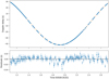 |
Fig. 1 Sample delay-advance curve of RXTE observations. The solid line represents the best fit. |
3.2 Orbital period decay
Similar to the modelling of the arrival times of the neutron star pulses, Eq. (1) can also be applied to model the binary epoch evolution and estimate the orbital period decay rate. In this case, the epoch En is given by
 (3)
(3)
Here E0 is the reference epoch for the orbital epoch history, and n is the orbit number. The first two terms of Eq. (3) describe the expected trend in the case of a constant orbital period. The last term describes the correction due to the orbital decay of the system.
In order to achieve better results for Porb and  , we opted to also include independently estimated binary epochs obtained from eclipse timing using the data from Swift/BAT alongside the epochs obtained in the last section, as well as the historical epochs from other authors (Table 2). The Swift/BAT light curves have a time resolution of 4888 s and are thus not suited for pulsar timing analysis. Instead, we analysed the light curves as a whole to calculate mid-eclipse times. The mid-eclipse times in general do not coincide perfectly with epochs determined from timing analysis since the epochs from the timing analysis correspond to T90, the time where the mean orbital longitude is 90°. For orbits with a non-zero eccentricity, the difference between T90 and the time of mid-eclipse is given by Eq. (2) in Falanga et al. (2015) as
 (4)
(4)
Based on the upper limit of the eccentricity from Raichur & Paul (2010b), we find, however, that the difference is at most ~5.7 s for Cen X-3, that is to say below the accuracy with which we can hope to determine individual mid-eclipse times. We assume, therefore, that those two types of epochs are to be the same going forward.
The mid-eclipse times for SwiftlBAT data were determined as follows. We first generated a template-folded orbital light curve by using all SwifiſBAT observations and assuming that the orbital period and period derivative are known (i.e. based on Raichur & Paul 2010b ephemerides). The mission-long light curve was then split into segments containing at least 50 orbital cycles, and data in each segment were folded with a constant period corresponding to expected value assuming ephemerides by Raichur & Paul (2010b). The folded profiles were then matched with a template using χ2 fitting in the same way as described above for pulsar timing analysis. The reference time tref,n for each profile was then calculated by using E0, Porb, and  from Raichur & Paul (2010b) and Eq. (3). Using the difference in spin phase between the template and profile, dϕn, and tref,n, the mid-eclipse time could then be calculated with
 (5)
(5)
An example of a fit can be seen in Fig. 2.
The obtained mid-eclipse times from Swift/BAT were combined with our results from the previous section as well as the historical epochs (Table 2). The observed-minus-calculated eclipse times as function of the orbit number can be seen in Fig. 3. The calculated eclipse times were calculated based on the ephemerides reported by Raichur & Paul (2010b) assuming no orbital decay. This curve was used to determine updated values of Рorb,  , and E0. To account for possible systematics, we utilised the Bayesian-nested Monte-Carlo sampling code BXA (Buchner 2016, 2019; Buchner et al. 2014) to obtain the final results for Porb,
  , and E0. Flat priors within a reasonable range (exceeding the estimated uncertainty of respective parameter values by a factor of ten) were used for each of the parameters. The results are summarised in Table 3, together with the values obtained by Raichur & Paul (2010b).
Cen X-3 orbital epoch history.
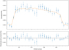 |
Fig. 2 Example of а Swift/BАТ light curve. The solid line represents the best fit with the template. |
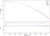 |
Fig. 3 Observed-minus-calculated eclipse times including Swift/BАТ data. The solid line represents our best fit to a constant orbital decay. |
Results of the nested Monte-Carlo sampling and corresponding values from Raichur & Paul (2010b).
3.3 Updated eccentricity limits
In order further push down the upper limit on the orbital eccentricity, we also performed a joint fit using the full binary epoch history, the Swift/BAT mid-eclipse times, and pulse arrival times obtained from observations of three orbital cycles most densely covered by observations. In particular, it is important that the observations of the selected cycles cover most of the orbital phases with a large number of uniformly distributed measured pulse arrival times. Following these criteria, we chose orbital cycles 4575, 4576, and 8146 for our analysis. Common parameters (axsin i, e, ω) between the cycles were linked to the corresponding parameter of the observation with the highest coverage of orbital phase, which in our case corresponds to cycle 4576. The T90 and orbital periods of the cycles were linked to the global orbital epoch history so that their estimated value for each individual orbital cycle uses all the available data. Free parameters for each individual orbital cycle were only the reference time for the spin parameters, that is t0 and the spin period p0 (we emphasise that all orbital parameters were also free to vary, and just linked between all cycles). A χ2 fit of this joint model was first carried out to obtain 3σ confidence bounds for model parameters, which were then used to define flat priors for the nested sampling. This procedure effectively allows one to exploit prior information on T90 for a particular orbital cycle given by the joint fit to long-term T90 evolution, and thus potentially decrease uncertainties for other orbital elements (including eccentricity).
We note that the Δχ2of some of the first 18 data points determined by Fabbiano & Schreier (1977) show a large deviation from the expected trend, which is consistent with results from other papers on the source (see e.g. Fig. 2 in Kelley et al. 1983). Since we cannot repeat the analysis for those orbital cycles as the data for those observations are no longer readily accessible, we attempted the following two approaches to assess the impact of these outlier points on the accuracy of our estimate. For the first approach we omitted the problematic data points, re-normalised the epoch history, and repeated the fit. For the next approach we increased the systematic of the epoch fit until we obtained a reduced χ2 of  . The results obtained by those three approaches to a joined fit are summarised in Table 4.
The results obtained from the epoch fit (Table 3) and from the initial joined fit of epoch history and individual cycles (Table 4) are consistent with each other considering uncertainties. However, results obtained by re-normalising the epoch history and increasing the systematic error (Table 4) do not completely agree with each other, and also show some deviation from the values reported in the literature. Indeed, with a difference of |Δporb| ~ 1.5 × 10⁻⁷, the determined orbital periods in Table 4 obtained by re-normalising the epoch history and including additional systematic uncertainty appear to differ from each other stronger what can be explained by the corresponding uncertainties. The period derivatives determined through both of these approaches are consistent with one another within the determined uncertainties, but inconsistent with the period derivatives determined through the other fits presented earlier.
Furthermore, the magnitudes of the orbital period, period derivative, and the eccentricity that were obtained by including an additional systematic uncertainty are larger than in the case of re-normalising the epoch history. It may be that the faster period decay and larger eccentricity are compensated for by a lower initial orbital period, which would then also explain the discrepancy between the orbital periods determined by the two approaches. Considering that the results for the eccentricity of the system obtained with the two approaches outlined above are also different, we cannot consider our results as a robust detection, but rather as an improved upper limit on the value of eccentricity. Based on our analysis, we therefore conclude that the eccentricity of the binary system is formally constrained between e = 0.00006 and e = 0.000266, and conservatively adopt the latter value as a conservative upper limit on its value.
Result of the three attempts at a joined analysis.
4 Discussion and conclusions
Cen X-3 is one of the few X-ray binaries where orbital decay is measured robustly. Measurements of the orbital period decay can be used to place limits on the mass transfer or mass-loss rate of the system (Deeter et al. 1981), and they are increasingly relevant in the context of the emerging field of gravitational-wave astronomy. The origin of the observed orbital decay rate in Cen X-3 can only be unambiguously identified if both the orbital period decay rate and eccentricity of the system are sufficiently well constrained. In this paper, we revisit this well-studied system, combining for the first time an extensive data set accumulated over the years with RXTE, HXMT, NuSTAR, and Swift/BAT observatories with the aim to accurately determine the values for the orbital period Porb and the period decay  . We estimate Porb = 2.087139842(18) d and a corresponding decay of
  days day−1, which is the most accurate estimate of those parameters to date. Furthermore, using a joint model consisting of the full binary epoch history and the pulse arrival times of several orbital cycles with significant coverage of the orbital phase, we were able to constrain the eccentricity of the system to 0.00006 ≤ e ≤ 0.000266. This estimate can be treated either as a tentative detection or, more conservatively, as an upper limit of the eccentricity in the system. With these newly obtained eccentricity limits, the period of a possible apsidal motion of the system can be determined. Using Eq. (10) in Thomas (1974) with an eccentricity of e = 0.00006, the apsidal motion period results in Paps ≃ 3.5 days. Using the upper limit of e = 0.000266 instead, one obtains an apsidal motion period of Paps ≃ 15 days. We therefore conclude that apsidal motion cannot be the cause for the observed apparent period decay of the system and the observed period decay has to be explained through other means. Assuming the change in orbital period is caused by conservative mass transfer with the neutron star accreting all matter lost by the companion, the rate of change of the orbital period is given by the following (van den Heuvel & de Loore 1973):

With an orbital period of Porb = 2.087139842 days, a rate of change of  days day−1, a neutron star mass of MN = 1.21 M⊙, and a companion mass of MC = 20.5 M⊙ (Ash et al. 1999), one therefore obtains roughly Ṁc = −7.784 × 10⁻⁷ M⊙ yr−1, which is slightly above the theoretical mass loss of Ṁc = −5.3 × 10⁻⁷ M⊙ yr−1 derived by Falanga et al. (2015) and considerably below the theoretical limit of Ṁc = −3 × 10⁻⁶ M⊙ yr−1 obtained by Wojdowski et al. (2001). If one instead considers non-conservative mass transfer, where the neutron star only accretes a fraction of the ejected matter, then following van den Heuvel & de Loore (1973),

where f is the fraction of accreted matter. Therefore, assuming the maximum theoretical mass loss of Ṁc = −3 × 10⁻⁶ M⊙ yr−1 derived by Wojdowski et al. (2001), we can estimate the fraction of mass accreted by the neutron star as f = 0.3, meaning 70% of the mass lost by the companion leaves the system.
This is in fact in line with the hypothesis that the mass loss and transfer in the system occur predominantly via strong stellar wind. The true cause of the observed decay is most likely a combination of multiple mechanisms and would require more accurate estimates of the mass-loss rate by the optical companion, and the accurate values of the orbital period, orbital period decay, and eccentricity reported in this paper should enable future investigations of the source to gain a deeper understanding of the mechanisms at play.
Acknowledgements
This work made use of the data from the HXMT mission, a project funded by China National Space Administration (CNSA) and the Chinese Academy of Sciences (CAS). This work has also made use of data and/or software provided by the High Energy Astrophysics Science Archive Research Center (HEASARC), which is a service of the Astrophysics Science Division at NASA/GSFC. We acknowledge the use of public data from the Swift data archive.
References
- Ash, T. D. C., Reynolds, A. P., Roche, P., et al. 1999, MNRAS, 307, 357 [NASA ADS] [CrossRef] [Google Scholar]
- Buchner, J. 2016, Stat. Comput., 26, 383 [Google Scholar]
- Buchner, J. 2019, PASP, 131, 108005 [Google Scholar]
- Buchner, J., Georgakakis, A., Nandra, K., et al. 2014, A&A, 564, A125 [NASA ADS] [CrossRef] [EDP Sciences] [Google Scholar]
- Chodil, G., Mark, H., Rodrigues, R., et al. 1967, Phys. Rev. Lett., 19, 681 [CrossRef] [Google Scholar]
- Deeter, J. E., Boynton, P. E., & Pravdo, S. H. 1981, ApJ, 247, 1003 [NASA ADS] [CrossRef] [Google Scholar]
- Fabbiano, G., & Schreier, E. J. 1977, ApJ, 214, 235 [NASA ADS] [CrossRef] [Google Scholar]
- Falanga, M., Bozzo, E., Lutovinov, A., et al. 2015, A&A, 577, A130 [NASA ADS] [CrossRef] [EDP Sciences] [Google Scholar]
- Giacconi, R., Gursky, H., Kellogg, E., Schreier, E., & Tananbaum, H. 1971, ApJ, 167, L67 [NASA ADS] [CrossRef] [Google Scholar]
- Howe, S. K., Primini, F. A., Bautz, M. W., et al. 1983, ApJ, 272, 678 [NASA ADS] [CrossRef] [Google Scholar]
- Kelley, R. L., Rappaport, S., Clark, G. W., & Petro, L. D. 1983, ApJ, 268, 790 [NASA ADS] [CrossRef] [Google Scholar]
- Krzeminski, W. 1974, ApJ, 192, L135 [NASA ADS] [CrossRef] [Google Scholar]
- Lecar, M., Wheeler, J. C., & McKee, C. F. 1976, ApJ, 205, 556 [NASA ADS] [CrossRef] [Google Scholar]
- Li, T.-P. 2007, Nucl Phys. B Proc. Suppl., 166, 131 [NASA ADS] [CrossRef] [Google Scholar]
- Murakami, T., Inoue, H., Kawai, N., et al. 1983, ApJ, 264, 563 [NASA ADS] [CrossRef] [Google Scholar]
- Nagase, F., Hayakawa, S., Kii, T., et al. 1984, PASJ, 36, 667 [NASA ADS] [Google Scholar]
- Nagase, F., Corbet, R. H. D., Day, C. S. R., et al. 1992, ApJ, 396, 147 [NASA ADS] [CrossRef] [Google Scholar]
- Raichur, H., & Paul, B. 2010a, MNRAS, 406, 2663 [NASA ADS] [CrossRef] [Google Scholar]
- Raichur, H., & Paul, B. 2010b, MNRAS, 401, 1532 [NASA ADS] [CrossRef] [Google Scholar]
- Schreier, E., Levinson, R., Gursky, H., et al. 1972, ApJ, 172, L79 [NASA ADS] [CrossRef] [Google Scholar]
- Schreier, E., Giacconi, R., Gursky, H., et al. 1973, IAU Circ., 2524, 1 [NASA ADS] [Google Scholar]
- Sparks, W. M. 1975, ApJ, 199, 462 [NASA ADS] [CrossRef] [Google Scholar]
- Swank, J. H. 1999, Nucl. Phys. B Proc. Suppl., 69, 12 [NASA ADS] [CrossRef] [Google Scholar]
- Thomas, H. C. 1974, ApJ, 191, L25 [NASA ADS] [CrossRef] [Google Scholar]
- Tuohy, I. R. 1976, MNRAS, 174, 45P [NASA ADS] [CrossRef] [Google Scholar]
- van den Heuvel, E. P. J., & de Loore, C. 1973, Nat. Phys. Sci., 245, 117 [NASA ADS] [CrossRef] [Google Scholar]
- van der Klis, M., Bonnet-Bidaud, J. M., & Robba, N. R. 1980, A&A, 88, 8 [NASA ADS] [Google Scholar]
- Wojdowski, P. S., Liedahl, D. A., & Sako, M. 2001, ApJ, 547, 973 [NASA ADS] [CrossRef] [Google Scholar]
- Zhang, S.-N., Li, T., Lu, F., et al. 2020, Sci. China Phys. Mech. Astron., 63, 249502 [NASA ADS] [CrossRef] [Google Scholar]
All Tables
Results of the nested Monte-Carlo sampling and corresponding values from Raichur & Paul (2010b).
All Figures
|
Fig. 1 Sample delay-advance curve of RXTE observations. The solid line represents the best fit. |
| In the text | |
|
Fig. 2 Example of а Swift/BАТ light curve. The solid line represents the best fit with the template. |
| In the text | |
|
Fig. 3 Observed-minus-calculated eclipse times including Swift/BАТ data. The solid line represents our best fit to a constant orbital decay. |
| In the text | |
Current usage metrics show cumulative count of Article Views (full-text article views including HTML views, PDF and ePub downloads, according to the available data) and Abstracts Views on Vision4Press platform.
Data correspond to usage on the plateform after 2015. The current usage metrics is available 48-96 hours after online publication and is updated daily on week days.
Initial download of the metrics may take a while.