| Issue |
A&A
Volume 628, August 2019
|
|
|---|---|---|
| Article Number | A108 | |
| Number of page(s) | 17 | |
| Section | Planets and planetary systems | |
| DOI | https://doi.org/10.1051/0004-6361/201935879 | |
| Published online | 14 August 2019 | |
Kepler Object of Interest Network
III. Kepler-82f: a new non-transiting 21 M⊕ planet from photodynamical modelling★
1
Institut für Astrophysik, Georg-August-Universität Göttingen,
Friedrich-Hund-Platz 1,
37077
Göttingen, Germany
e-mail: jfreude@astro.physik.uni-goettingen.de
2
Stellar Astrophysics Centre, Aarhus University,
Ny Munkegade 120,
8000
Aarhus, Denmark
3
Department of Earth and Planetary Sciences, Weizmann Institute of Science,
Rehovot
76100, Israel
4
Astronomy Department, University of Washington,
Seattle,
WA
98195, USA
5
Virtual Planetary Laboratory, University of Washington,
Seattle,
WA
98195, USA
6
Rosseland Centre for Solar Physics, University of Oslo,
PO Box 1029
Blindern,
0315 Oslo, Norway
7
Institute of Theoretical Astrophysics, University of Oslo,
PO Box 1029
Blindern,
0315 Oslo, Norway
8
Amazon Web Services,
Seattle,
WA
98121, USA
9
Aix-Marseille University, CNRS, CNES, LAM,
Marseille,
France
10
Universidad de La Laguna, Departamento de Astrofísica,
38206
La Laguna, Tenerife, Spain
11
Leibniz-Institut für Astrophysik Potsdam, An der Sternwarte 16,
14482
Potsdam, Germany
12
Astrophysics Research Centre, Queen’s University Belfast,
Belfast
BT7 1NN, UK
13
Institut de Ciències de l’Espai (IEEC-CSIC), C/Can Magrans, s/n, Campus UAB,
08193
Bellaterra, Spain
14
Institut d’Estudis Espacials de Catalunya (IEEC), Gran Capità,
2-4, Edif. Nexus,
08034
Barcelona, Spain
15
Institute for Astronomy, Astrophysics, Space Applications and Remote Sensing, National Observatory of Athens, Metaxa & Vas. Pavlou St., Penteli,
Athens, Greece
Received:
13
May
2019
Accepted:
20
June
2019
Context. The Kepler Object of Interest Network (KOINet) is a multi-site network of telescopes around the globe organised for follow-up observations of transiting planet candidate Kepler objects of interest with large transit timing variations (TTVs). The main goal of KOINet is the completion of their TTV curves as the Kepler telescope stopped observing the original Kepler field in 2013.
Aims. We ensure a comprehensive characterisation of the investigated systems by analysing Kepler data combined with new ground-based transit data using a photodynamical model. This method is applied to the Kepler-82 system leading to its first dynamic analysis.
Methods. In order to provide a coherent description of all observations simultaneously, we combine the numerical integration of the gravitational dynamics of a system over the time span of observations with a transit light curve model. To explore the model parameter space, this photodynamical model is coupled with a Markov chain Monte Carlo algorithm.
Results. The Kepler-82b/c system shows sinusoidal TTVs due to their near 2:1 resonance dynamical interaction. An additional chopping effect in the TTVs of Kepler-82c hints to a further planet near the 3:2 or 3:1 resonance. We photodynamically analysed Kepler long- and short-cadence data and three new transit observations obtained by KOINet between 2014 and 2018. Our result reveals a non-transiting outer planet with a mass of mf = 20.9 ± 1.0 M⊕ near the 3:2 resonance to the outermost known planet, Kepler-82c. Furthermore, we determined the densities of planets b and c to the significantly more precise values ρb = 0.98−0.14+0.10 g cm−3 and ρc = 0.494−0.077+0.066 g cm−3.
Key words: planets and satellites: dynamical evolution and stability / planets and satellites: detection / methods: data analysis / techniques: photometric / stars: individual: Kepler-82 / stars: fundamental parameters
Ground-based photometry is only available at the CDS via anonymous ftp to cdsarc.u-strasbg.fr (130.79.128.5) or via http://cdsarc.u-strasbg.fr/viz-bin/qcat?J/A+A/628/A108
© ESO 2019
1 Introduction
There is no doubt about the impact that the Kepler Space Telescope has had on the exoplanetary field. Among many other outstanding and benchmark contributions, such as the first possibly habitable planet with known radius (Borucki et al. 2012), and the first exoplanet ever found with two suns in its sky (Doyle et al. 2011), Kepler data have allowed us to characterise planetary masses via transit timing variations (TTVs, see e.g. Fabrycky et al. 2012; Mazeh et al. 2013; Steffen et al. 2013). Nonetheless, after four years of continuous monitoring of the same field of view, the nominal observations of Kepler came to an end. This left several Kepler objects of interest (KOIs) without a proper characterisation, even though they presented large amplitude TTVs in the Kepler data alone. To continue with the successful characterisation of planetary masses of KOIs via TTVs, we have organised the Kepler Object of Interest Network1 (KOINet). To date, results of our network comprise KOINet’s first light (von Essen et al. 2018), and the in-depth photodynamical characterisation of Kepler-9b/c (Freudenthal et al. 2018). While in the former we demonstrated KOINet’s strategy and functionality, along with initial results on four KOIs, in the latter we were able to determine values for the planetary densities that are the most precise measurements in the regime of Neptune-like exoplanets. Furthermore, we predicted that the transits of Kepler-9c would disappear in about 30 yr. These results arose from the combinationof the Kepler long- and short-cadence data with KOINet follow-up transit observations, along with a comprehensive and coherent analysis carried out with our photodynamical modelling. Similar analyses have likewise revealed precise planetary densities for other systems, like Kepler-117 by Almenara et al. (2015), K2-19 by Barros et al. (2015), WASP-47 by Almenara et al. (2016), Kepler-138 by Almenara et al. (2018a), and Kepler-419 by Almenara et al. (2018b). In many of these cases the authors also demonstrated consistent planetary mass determinations from TTV and radial velocity (RV) measurements.
From amongst our KOINet targets we pinpointed Kepler-82 (KOI 0880) as an interesting system that deserves a detailed photodynamical analysis. The Kepler-82 system contains a total of four confirmed transiting planets. The two inner planets have periods of Pd = 2.38 d and Pe = 5.90 d, which were confirmed by Rowe et al. (2014). The two outer planets have a period ratio close to 2:1 with Pb = 26.44 d and Pc = 51.54 d. This commensurability of the periods results in strong TTVs (see Fig. 1), which led to the confirmation of the two outer planets a year before the inner planets (Xie 2013). The inner two planets are not much affected by this dynamical interaction and also show no measurable dynamical interaction with one another. Yet Kepler-82e shows TTVs with an amplitude of about 15 min, where the uncertainties of the transit times are of the same order, and the variations are without significant periodicity (Holczer et al. 2016). Ofir et al. (2018) found TTVs in Kepler-82d with an amplitude of  min and a frequency peak that just surpassed their significance criteria. The peak does not correspond to any expected dynamical frequency.
The first characterisation of the Kepler-82b/c TTVs was carried out by Xie (2013). The author found the TTVs to be sinusoidal as expected for near 2:1 mean-motion resonance (MMR) systems. In contrast with many other similar systems, the sinusoidal-shaped TTVs of both planets are not anti-correlated; instead the phase difference is close to zero. The author calculated the nominal masses assuming a two-planet system and found a relatively large mass ratio of mb ∕mc ~ 100.6 ~ 4, which means a very large density ratio of  . Another nominal mass computation by Hadden & Lithwick (2014) indicates a smaller mass (~ 3) and density ratio (~7).
A further characterisation was done by Ofir et al. (2018) by analysing periodograms of the TTVs of Kepler-82b/c. They found the most significant peak in the periodogram of Kepler-82b fits the 2:1 MMR super frequency. However, the highest amplitude peak of Kepler-82c is notably offset from the highest peak of Kepler-82b and the 2:1 MMR super frequency. Additionally, they found one other significant peak for Kepler-82b and three in Kepler-82c.
The following work includes the first dynamical analysis of the Kepler-82b/c system. We applied a photodynamical model to Kepler data and ground-based follow-up observations from KOINet. With this we were able to constrain the planetary masses more precisely, and by including another non-transiting planet, most of the frequency peaks, can be explained. Furthermore, we were able to determine the stellar mass, radius and age from our results by combining the modelled stellar densities with spectroscopic values and comparing these values with stellar evolution models.
The paper is structured as follows. The data acquisition and treatment within the KOINet is described in Sect. 2. We present our own implementation of a photodynamical model in Sect. 3. The detection of a third dynamically important non-transiting planet in the TTVs of Kepler-82c is described in detail in Sect. 4. The results from the analysis are discussed in Sect. 5. We end the paper with a conclusion in Sect. 6.
2 KOINet data
In order to organise the KOINet observations we calculated transit time predictions from the Kepler observations as described in Sect. 2.5 of von Essen et al. (2018). In the case of Kepler-82b, a linear plus sine function was fitted to predict future times of transit. For Kepler-82c we provided two different predictions. One coming from a sine plus linear fit, and one from fitting a parabolic function as a turnover to the sine curve was not measured by the Kepler observations. The low precision in the transit time predictions of Kepler-82c in particular led to only a small fraction of KOINet Kepler-82 light curves with transits included. Between 2014 and 2018 eleven light curves of Kepler-82 were obtained, while only three of them show transit signals of Kepler-82b/c.
Table 1 lists the main characteristics of the data presented in this paper, such as the observing telescope and the observation dates the precision of the data, the total duration of the observation, and the transit coverage. To increase the photometric precision of the collected data, we have, when possible, slightly defocused the telescopes (Kjeldsen & Frandsen 1992; Southworth et al. 2009). Below is a brief description of the main characteristics of each of the telescopes involved in this work.
The Apache Point Observatory hosts the Astrophysical Research Consortium 3.5 m telescope (henceforth “ARC 3.5 m”), and is located inNew Mexico, United States of America. The photodynamical analysis of Kepler-82 presented here includes one light curve taken with the ARC 3.5 m during our first observing campaign in 2014.
The 2.5 m Nordic Optical Telescope (NOT 2.5 m) is located atthe Observatorio Roque de los Muchachos in La Palma, Spain. Currently, telescope time for KOINet is assigned via a large (three-years) program. Here, we present two light curves taken between the fourth and fifth observing seasons.
The 80 cm telescope of the Instituto de Astrofísica de Canarias (IAC 0.8 m) is located at the Observatorio del Teide, in the Canary Islands, Spain. The one transit light curve obtained in the first season of KOINet suffered from technical difficulties during the night. For this reason the resulting science frames were corrupted and, thus, it was impossible for us to properly reduce them.
The Oskar Lühning Telescope (OLT 1.2 m) has a 1.2 m aperture diameter and is located at the Hamburger Observatory in Hamburg, Germany. Kepler-82 was observed for one night in the first season of KOINet with OLT 1.2m. Unfortunately, the observation taken in 2014 suffered from technical difficulties.
The Telescopi Joan Oró is a fully robotic 80 cm telescope (TJO 0.8 m) located at the Observatori Astronomic del Montsec, in the north-east of Spain. The parabolic prediction of Kepler-82c was chosen as transit time for an observation. The obtained observation contains only off-transit data.
The fully robotic 2 m Liverpool telescope (LIV 2 m; Steele et al. 2004) is located at the Observatorio Roque de los Muchachos and is owned and operated by Liverpool John Moores University. During the second season of KOINet a transit time predicted from parabolic TTVs was chosen for an observation. The resulting light curve does not contain a transit.
The Centro Astronómico Hispano-Alemán hosts, among others, a 2.2 m and a 3.5 m telescope (“CAHA 2.2 m” and “CAHA 3.5 m”). An observation was taken with each telescope. No transit is present in the light curves.
The MMT observatory, a joint venture of the Smithsonian Institution and the University of Arizona, is located on the summit of Mt. Hopkins in south-eastern Arizona, USA. The telescope has a collecting area of 6.5 m (SAO 6.5 m). The data collected with this telescope were of sub-millimagnitude precision, but taken outside transit due to bad scheduling decisions.
The National Observatory of Athens hosts the 1.2 m Cassegrain telescope of the Astronomical Station Kryoneri (KRYO 1.2 m). For the last 40 yr the telescope has been operational, with an extensive upgrade taking place in 2016. Data collected with this telescope were of good quality, however taken outside transit.
All collected observations underwent the KOINet reduction pipeline, and a preliminary analysis for deriving reliable errorbars and the detrending components. This process is described in von Essen et al. (2018) and Freudenthal et al. (2018).
Characteristics of collected ground-based transit light curves of Kepler-82b/c, collected through KOINet.
3 The photodynamical model
For the KOINet data analysis we developed a simultaneous transit light curve model for all observations of each system that takes the system dynamics into account. This allows us to determine the planetary masses in addition to the transit parameters. A full description of our photodynamical model can be found in Freudenthal et al. (2018). Briefly, we combine a numerical integration of the whole system over the time span of observations, and from the output sky positions (projected distance of each planet to the star) we calculate the transit light curve. We use a second-order mixed-variable symplectic (MVS) algorithm to perform the numerical integration as implemented in our python-wrapper for mercury6 (Chambers 1999). The integrator is complemented by first-order post-Newtonian correction (Kidder 1995), and we correct the individual times for the light-travel-time effect for each planet. From the numerical integration of the system we extract the planet-to-star centre distances to calculate the light curve through the transit model of Mandel & Agol (2002). Here we use the occultquad routine with the quadratic limb-darkening law implemented.
As in Freudenthal et al. (2018), the numerical integration is done on a coarse grid, and only in the vicinity of transits is the integration refined with a time step of 0.01 d. The coarse grid is optimised to give the shortest possible computation time with sufficient accuracy. For this system a time step of a hundred-twentieth of the period of the innermost included planet was used. For long-cadence data we take the finite integration time into account (Kipping 2010). Hence, we compute the transit light curve with a time step of ~ 1 min and rebin it to the cadence of the data points.
Our photodynamical model is coupled to the Markov chain Monte Carlo (MCMC) emcee3 algorithm (Foreman-Mackey et al. 2013). All fitting parameters have uniform priors with broad boundaries chosen to avoid non-physical results. A detailed description of the model parameters can be found in Freudenthal et al. (2018). To summarise, the model requires the mass, m, and the radius R of the central star, as well as the two quadratic limb darkening coefficients, c1 and c2, that reflect the wavelength response of the optical setup of each telescope per instrument, and per planet, p (p ∈ {b, c, f} from Sect. 4 and for example in the Tables 2 and A.2) the parameters are described below.
A mass ratio is needed. For the innermost planet the ratio to the central star, m1 ∕mS, is taken and for all other planets the ratio to the next inner one,  . Secondly, a parameter to calculate the semi-major axis, a, is needed. In the case of transiting planets it is calculated from the mean period, Pp and as a free parameter a correction factor, ap,corr:
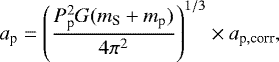
with the gravitational constant, G. We fitted a linear ephemeris T = ΔTp,0 + Pp × n to the transit times, T, giving us the mean period Pp and an offset ΔTp,0. For non-transiting planets the semi-major axis is calculated from the period given by a period ratio to the next inner planet. Furthermore, the eccentricity, ep, is needed. The orbital angles, inclination, ip, argument of the periastron, ωp, and the longitude of the ascending node, Ωp, are needed. Whereas the latter is fixed to zero for the innermost planet, the other values are given relative to the innermost planet. The instantaneous position of the planets at a given reference time needs to be defined. We take the mean anomaly, Mp, as measurement for the position of each planet. This angle is calculated from the mean period, Pp, as well as the offset, ΔTp,0. As a free parameter, we have an addition to this derived mean anomaly, Mp,corr:
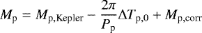
with the mean anomaly at transit time calculated for a Kepler orbit from the argument of periastron and eccentricity, Mp,Kepler, and the second term is giving the difference between the mean anomaly at transit time and the mean anomaly at the starting time of the integration. That means the free parameter Mp,corr is giving thecorrection from a pure Keplerian orbit due to the interaction with the other planets. Lastly, The planet-to-star radius ratio, Rp ∕RS, only for transiting planets needs to be given.
We treated Kepler data and ground based observations of KOINet as the description in Freudenthal et al. (2018). From Kepler photometry we extracted the transit duration symmetrically around each transit mid point four times. To account for intrinsic stellar photometric variability we normalised each transit light curve dividing it by a time dependent second-order polynomial optimised on the off-transit data points. The coefficients of this parabola are derived through a simple least-squares minimisation routine. As previously mentioned, for long-cadence data, the photodynamical light curve model is oversampled by a factor of 30 and rebinned to the actual data points. This procedure is not necessary for short-cadence data. The high signal-to-noise ratio (S/N) of Kepler data allows us to include the quadratic limb darkening coefficients into our free parameters set. This allows for a more realistic inclination and star and planetary radii determination due to the good constrained transit shape.
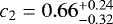
Due to the lower S/N of the ground-based data, we fixed the quadratic limb darkening coefficients to values which are derived as described in von Essen et al. (2013) from stellar parameters for the Johnson–Cousins R-band filter, which we used for all of our observations. For stellar parameters closely matching the ones of Kepler-82 (Petigura et al. 2017), the derived limb darkening coefficients are c1 = 0.52 and c2 = 0.14. The best-matching coefficients of the detrending components, derived during the first data analysis (in Sect. 2), for each ground-based observation are calculated as a linear combination at each call of the photodynamical model.
4 Dynamical analysis of Kepler-82
In the following sections we outline the detection of a fifth, non-transiting planet in the Kepler-82 system, which is required to explain the available data. We call the planet Kepler-82f hereafter.
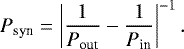
In this work we analyse the transit light curves of the outer two planets of Kepler-82, b and c. These planets have a period ratio close to the 2:1 resonance. The inner two, d and e, show no strong TTV amplitudes and especially no frequencies due to interaction with the outer two (Ofir et al. 2018). In a first step we determined the transit times from long-cadence Kepler data with the procedure described in Sect. 4.1 of von Essen et al. (2018). In addition to the near resonant interaction with Kepler-82b, the transit times of Kepler-82c show a strong “chopping” component, which is visible by a sudden jump in the transit time following every three consecutive transits which show drifting transit times. The period of chopping is controlled by the times between conjunctions of planet c and the fifth planet, given by the synodic period
Since the jump in chopping is seen every three transits of planet c, this indicates that the synodic period is either 3 × Pc or 3∕2 × Pc, which would give a dependency of the acceleration and the deceleration during the orbits of the inner planet from three times its period. These synodic periods can be created by an outer planet near the 3:2 or 3:1 resonance with planet c. Based on the synodic period of planet c, an inner planet near the 3:4 or 3:5 resonance would also be possible; however, such a planet would be near a 3:2 or 6:5 resonance with Kepler-82b, and would then induce a strong signal in its TTVs. Such a TTV signal is not measured; hence the fifth planet must orbit exterior to planet c.
For this reason we optimised the parameters of the two outer unknown planet configurations (from now on the 3:2:1 and 6:2:1 resonance models, for convenience we skip the more accurate notation of the planets being near resonant) in a photodynamical model applied to the Kepler long-cadence (quarters 1–6) and short-cadence (quarters 7–17) data. From the Kepler data alone, both of the resonance models show the same probability. The prediction for the transit times, however, start to diverge rapidly after the Kepler mission terminates, as visualised in Fig. 1. The figure shows the transit times with a linear ephemeris subtracted (observed minus calculated, thus henceforth, O–C diagram) of Kepler-82b at the top and of Kepler-82c at the bottom. For Kepler-82b the models start to differ within 3σ by the end of 2015 and for Kepler-82c by mid 2014. The three KOINet transit light curves (plotted in Fig. 2; in the O–C diagram the transit times are indicated in red) show a clear preference for the 3:2:1 resonance model. In addition, the latest KOINet observation where no transit is measured clearly contradicts the 6:2:1 resonance model prediction.
On this account we re-optimised the 3:2:1 resonance model parameters to the Kepler data complemented by the three KOINet transit light curves. The resulting planetary and stellar parameters from this fit can be found in Table 2. Table A.2 lists the planetary and stellar parameters from all model optimisation done in this work. The tables shows from top to bottom the modelled and derived values of Kepler-82b, Kepler-82c, the new planet, Kepler-82f, and the central star. The osculating orbital elements are given at the reference time BJD = 2 454 933.0, 100 days later than the standard Kepler reference time (BKJD).
For comparison we also optimised the transiting 2-planet system (2:1 resonance model) on the Kepler long- and short-cadence data. The results are listed as well and presented in the O–C diagram (Fig. 1) as grey areas.
4.1 Details of optimisation
We initially optimised the different planetary system models (described later in this section) on the transit times, fixing all transit shape determining parameters to narrow the parameter space for the photodynamical analysis. We used the median values and the 3σ interval of this analysis for a Gaussian random choice of starting parameter sets. The parameters describing the transit shape – the inclination, limb darkening coefficients and planet and star radii – are taken from the individual transit fits.
We fixedthe stellar mass to its literature value of mS = 0.91 M⊙ (Johnson et al. 2017) during the TTV and the photodynamical analysis. The uncertainty on the stellar mass,  , is applied to the derived parameters that depend on it via error propagation. In particular this affects the planetary masses, semi-major axes, and periods.
Optimising a linear ephemeris to the Kepler transit times of Kepler-82b/c, we obtained the offsets ΔTb,0 = 41.23683 d and ΔTc,0 = 22.52550 d as intercepts, and the mean periods Pb = 26.44404770 d and Pc = 51.53912652 d as slopes. The offsets and mean periods are used for the determination of the semi-major axes and the mean anomalies, as described previously in Sect. 3.
The properties of all of the photodynamical model optimisation procedures on the transit light curves are given in Table 3. Listed are the parameters as follows. In the first row the number of walkers used for extracting the final results are given. We initialised with more walkers; however, a variable number of walkers ended in higher χ2 minima. Next, the number of iterations we obtained per walker are given, followed by the number of iterations we used as initial burn-in. From the MCMC posterior distribution we calculated the autocorrelation length according to Goodman & Weare (2010), but averaging over the autocorrelation function per walker instead of averaging directly over the walker values, as discussed in the blog by Daniel Foreman–Mackey2. The given autocorrelation length allows us to derive the effective number of individual samples. The last two rows contain the degree of freedom (d.o.f.) of the optimisation and the best reduced χ2 value. We note a significant deviation from one in the reduced χ2 values which is unexpected considering the high dof numbers. For this reason, we quadratically add a systematic error of  to the model parameter uncertainties in Tables 2 and A.2.
While optimising the 3:2:1 resonance model we realised that we could actually derive the entire orbit of the non-transiting planet. By this we mean that we could constrain the inclination – which avoids transit – and the other orbital angles: the longitude of periastron, the longitude of ascending node, and the mean anomaly. We found two different configurations with ib constrained to below 90°. The first has ic < 90° and if >90° (henceforth configuration I), the second isthe opposite with ic > 90° and if < 90° (configuration II). The configurations are visualised in Fig. 3, where the impact parameter of the planets is plotted against the distance to the star. The values and uncertainties are derived from 1000 randomly chosen results from modelling the Kepler and KOINet data in configuration I in red and in configuration II in blue. Both configurations have the same probability and are equivalent in all other parameters. This means that the transit time predictions and shape are the same for both configurations. The other two configurations, with either both planets having inclinations below 90° or both above 90°, are not chosen by the MCMC optimisation, although allowed and included in the starting positions of the walkers. We modelled both configurations individually with the same number of iterations and combined all resulting walkers to extract the results. Given that the KOINet transit times are located at the 3:2:1 resonance model predictions, we optimised this model on these light curves together with the Kepler data again in both of the configurations.
Following this detection we also set the inclination of the non-transiting planet in the 6:2:1 resonance model as a free parameter. In this case the inclination did not avoid the transit region, though it spans a large area where the majority of solutions is in the non-transiting region (about 88% in a conservative calculation of the impact parameter b). Nonetheless, we inspected the Kepler data for these transits. Based on the mass ratio to Kepler-82c of  we can expect transits of larger depths compared with the other system’s planets. Such transits are not detected.
 |
Fig. 1 O–C diagrams of Kepler-82b at the top and Kepler-82c at the bottom with transit times from modelling the transits individually. The black points refer to the transit data from the Kepler telescope. The red points are the individual transit times from the new KOINet observations (plotted in Fig. 2). The violet lines show observed epochs but with non-detections of transit. The green area indicates the 99.7% (light) and the 68.3% (dark) confidence interval of the 6:2:1 resonance model optimised on Kepler long- and short-cadence data only, derived from 1000 randomly chosen models out of the MCMC posterior distribution; the green line is the median. The blue areas indicate the 3:2:1 resonance model solution. The grey areas present the 2:1 resonance model. |
 |
Fig. 2 KOINet transit light curves of Kepler-82. The three transit light curves (black) are overplotted with 1000 random models of the 3:2:1 resonance optimised using Kepler long- and short-cadence data (red) and including these KOINet observations(blue). |
4.2 Results
Along with the optimised parameters listed in Tables 2 and A.2 we display the KOINet transit light curves in Fig. 2 in black. These are overplotted with 1000 model solutions randomly chosen from the MCMC posterior distribution from analysing only Kepler data in red, and including these KOINet transit light curves in blue with the 3:2:1 resonance model. Similar to the O–C plot in Fig. 1 we show the TTV behaviour for the 3:2:1 resonance model optimised on all available transit light curves in comparison to the optimisation on Kepler data only in Fig. A.1. Including the KOINet transit observations led to a narrowing of the transit time predictions of Kepler-82c (visible in the Figs. 2 and A.1) and the shrinkage of the mass uncertainties of Kepler-82b (see Table A.2). The transit time predictions for the next fifteen years are listed in Table A.1. Finally, the parameter correlations are visualised in a corner plot in Fig. A.3.
5 Discussion
The most prominent signal in the TTVs of the Kepler-82b/c system is the dynamical interaction with each other due to its near 2:1 resonance configuration. Xie (2013) calculated nominal masses from the amplitudes of these TTVs and a derived stellar mass from logg and RS under the assumption of a 2-interacting-planet system. Their derived masses for Kepler-82b/c are  and
and 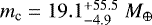 , respectively.Additionally, they derive the planetary radii from single transit fitting to Rb = 4.00 ± 1.82 R⊕ and Rc = 5.35 ± 2.44 R⊕. With these values they propose a density ratio of ~10 for the planets. In an initial model we tested this 2-planet system with our photodynamical analysis. We found planetary masses and radii with much smaller uncertainties (see Table A.2) that agree within their errorbars with the values calculated by Xie (2013). The density ratio of our result is even higher with ρb ∕ ρc ~ 14.
The stellar parameters of this analysis show significant deviations from literature values that are derived by spectroscopic observations. The stellar radius with 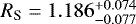 is more than 1σ higher than the measurement by Johnson et al. (2017) (
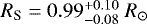 ) and the quadratic limb darkening coefficients calculated by Claret & Bloemen (2011; ATLAS model) to c1 = 0.4695 and c2 = 0.2240 do not fall within the modelled values (
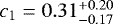 ,
,  ).
).
These stellar parameters as well as the planetary masses, and with these the densities, become more plausible in their values when including a third planet in the dynamical analysis. The signal of such a planet is clearly visible in the TTVs of Kepler-82c as a jump every three consecutive transits (see Fig. 1). As explained in Sect. 3, two different configurations of a three-planet system can explain this chopping effect in the Kepler data. Both of these include another outer non-transiting planet, near the 3:1 or 3:2 period resonance to Kepler-82c. Including either of these planets dramatically reduces the mass of Kepler-82b, and thus also reduces the ratio of the density Kepler-82b to c. Both system models are very similar in probability for Kepler data, the 6:2:1 resonance model has a slightly higher  than the 3:2:1 resonance system. With KOINet data we were able to distinguish between these two models. The detected transits fall at the 3:2:1 model prediction, and one of the observations where no transit is observed precludes the 6:2:1 model predicted transit time. In the following we refer to the 3:2:1 resonance model solution on Kepler and KOINet data when not differently specified.
The density ratio of the resulting Kepler-82b/c planets reduces to a factor of ~ 2. Such a ratio is no longer very unusual; the values are discussed in the context of the literature below by visualising them in a mass-radius diagram. The density of the new planet can not be determined as, due to the lack of transits, the radius is not measurable. In addition, the stellar radius and the limb darkening values fit in with the literature values within 1σ-uncertainty.
At the same time the predicted RV signal reduces from an amplitude of ~ 50 m s−1 for the 2-planets system to about ~7.5 m s−1 for the 3-planets system near 3:2:1 resonance. With Kepler-82 being a relatively faint star (Kp = 15.158), such a signal is not measurable with current instruments.
Planetary and Stellar parameters from photodynamical analysis of the 3:2:1 resonance model on Kepler data and the three KOINet transit light curves.
5.1 Previously proposed planets
Bovaird et al. (2015) predicted two additional planets in the Kepler-82 system with periods of 11.8 ± 2.0 days and 120 ± 20 days based on the Titius–Bode relation. Neither the new planet proposed here near the 3:2 resonance to Kepler-82c, nor the less viable option with a planet near the 3:1 resonance, matches the position of one of the predicted planets. The predicted outer planet is in between the two possibilities within 3σ distance to each of them.
5.2 Dynamical stability
Subsequent to the photodynamical analysis we tested the dynamical stability of the modelled systems. With the same integrator, the second-order mixed-variable symplectic algorithm implemented in the mercury6 package by Chambers (1999), we extend the numerical simulation of the best found solution for each system configuration to 10 Gyr. For this application the post-Newtonian correction (Kidder 1995) was implemented as well. The integration is done with a time step size of 1 day which is roughly a twentieth of the innermost planet considered in our analysis (Kepler-82b). This gives a good compromise between a sufficient sampling for small integration errors and a reasonable computation time. We tested the stability of the 2:1 resonance 2 planets solution, the 6:2:1 resonance system as well as the 3:2:1 resonance 3 planets model that is preferred by the KOINet data. All of these system configurations survived the 10 Gyr integration; only the 2-planet system showed chaotic parameter evolution. A closer inspection of the 6:2:1 resonance system long-term behaviour showed that given this model we are observing the transiting planets b and c at a minimum in periodically changing eccentricities. The values are ranging in roughly eb = 0.002−0.08 and ec = 0.004−0.06. The probability for the planets to be in this minimum at observation time is below 10%, making this scenario even less likely.
Another indication for stability is the planets to be near resonant, but not in resonance. We checked that the modelled planets are not in resonance through calculating the resonant angles (Morbidelli 2002), as well as the Laplace resonant angle. All angles are circulating and do not librate, which would be the sign for the planets to be in resonance.
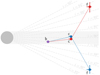 |
Fig. 3 Configurations of the Kepler-82 system. With the star in grey on the left side and the observer on the right side this shows the two different configurations: b in violet has the same position in both, c and f in red shows configuration I and in blue configuration II. The grey area indicates the region of impact parameters below one. The distances are not true to scale with the stellar radius, therefore a few inclination values are indicated as dashed grey lines. A similar plot with true scales can be found in Fig. A.2. |
Properties of the optimisation of different models paired with different data sets.
Comparison between TTV inducing frequencies calculated from periods of the system solution to measured TTV frequencies by Ofir et al. (2018).
5.3 TTV frequencies
The frequencies in the TTVs of the Kepler-82 system were analysed by Ofir et al. (2018). In the TTVs of Kepler-82b they found, besides the main peak at  , another significant frequency peak at (101.5 ± 2.8) × 10−4 d−1. The main frequency peak of Kepler-82c is at (8.15 ± 0.12) × 10−4 d−1. In addition to that they found three more peaks in the TTVs at ((17.9, 58.9, 68.9) ± 3.2) × 10−4 d−1. Except for the main peak of Kepler-82b belonging to the super frequency of the near 2:1 resonance with Kepler-82c, they could not explain the detected frequencies with super frequencies of all of the mean motion resonances, orbital frequencies, chopping frequencies, or stroboscopic frequencies of the confirmed planets in the system.
In the same manner we computed the super frequencies of all mean motion resonances, orbital frequencies, and chopping frequencies of our resulting system from photodynamical analysis. The calculated frequencies are listed in Table 4. With the exception of two measured frequencies, we can explain them with interactions of the planets in the modelled system. Significantly, the super frequencies from mean motion resonances, expected to induce TTV signals, match the significant peaks found by Ofir et al. (2018). The super frequency of Kepler-82b/c corresponds to the main peak in the TTVs of Kepler-82b. Kepler-82c/f have a super frequency that explains the main peak of the TTVs in Kepler-82c. And finally, the super frequency of Kepler-82b/f matches a significant peak in the TTVs of Kepler-82c. Additionally the chopping frequency of Kepler-82c/f explains another peak of Kepler-82c TTVs. Two of the Ofir et al. (2018) frequencies with smaller confidence remain unexplained, these are the (101.5 ± 2.8) × 10−4 d−1 frequency in planet b and the (68.9 ± 3.2) × 10−4 d−1 frequency inplanet c.
For comparison, we computed the same frequencies from the 6:2:1 resonance results. In this case the super frequency of Kepler-82b/c matches, as expected, with the main peak of the Kepler-82b frequencies, and the orbital frequency of the third non-transiting planet matches the (58.9 ± 3.2) × 10−4 d−1 peak. Besides these, no other matching frequencies were found, especially the main peak in the TTVs of Kepler-82c is not explained.
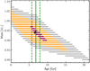 |
Fig. 4 Mass-age diagram of Kepler-82 from MESA stellar evolution models (MIST). The black star and the red, orange, and grey dots correspond to the best matching value and the 1σ, 2σ, and 3σ areas derived from results on the density of the whole set photodynamical modelling and from the literature values of the effective temperature, the surface gravity, and the metallicity by Petigura et al. (2017). The gyrochronologic age is indicated in green by a solid line and its 1σ range as dashed lines. |
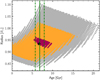 |
Fig. 5 Radius-age diagram of Kepler-82 from MESA stellar evolution models (MIST). The black star and the red, orange, and grey dots correspond to the best matching value and the 1σ, 2σ, and 3σ areas derived from results on the density of the whole data set photodynamical modelling and from the literature values of the effective temperature, the surface gravity, and the metallicity by Petigura et al. (2017). The gyrochronologic age is indicated in green by a solid line and its 1σ range as dashed lines. |
5.4 Stellar parameters
Transit measurements provide the information about the stellar density (Agol & Fabrycky 2018). In our photodynamical analysis we decided to model the stellar radius while fixing the stellar mass. With this parameterisation, the density is modelled as well. We derived the stellar radius to be 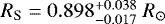 . The high asymmetry in the uncertainties is attributed to the symmetry of the inclination of Kepler-82c around 90°. Together with the stellar mass from Johnson et al. (2017) of mS = 0.91, this results in a stellar density of
 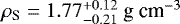 .
.
With this photodynamical-determined density and the measured stellar parameters (Petigura et al. 2017,from HIRES observations within the California–Kepler Survey) of the effective temperature Teff = 5400.5 ± 60 K, the surface gravity logg = 4.372 ± 0.100, and metallicity Fe/H = 0.201 ± 0.040 we modelled the stellar radius, mass, and age with stellar evolution models. We extracted the corresponding values from MESA (Paxton et al. 2011, 2013, 2015) evolutionary tracks interpolated by MIST (Dotter 2016; Choi et al. 2016), rejecting values of the very early evolution below 0.1 Gyr. The results are visualised in Fig. 4 as a mass-age diagram and in Fig. 5 as a radius-age diagram with the best-matching value and the 1σ, 2σ, and 3σ areas as a black star and red, orange and grey dots respectively. For comparison, the gyrochronological stellar age derived below is plotted in green; it fits within the 1σ errorbars. The stellar parameters are derived to be 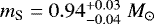 for the mass,
 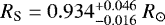 for the radius, and a stellar age of
 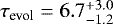 Gyr.
Gyr.
We corrected the photodynamically-determined parameters that depend on stellar mass and radius, namely planetary masses, semi-major axes, and radii, with these newly determined values. The corrected values are listed in column six of Table A.2. The planetary masses and radii of Kepler-82b/c are compared in Fig. 6 with literature values of planets with masses up to 20 M⊕ from The Extrasolar Planets Encyclopaedia3.
For testing the results of the stellar evolution model analysis we applied the gyrochronologic age determination method to the Kepler-82 system. Therefore we determined its rotation period from the Kepler long-cadence photometry excluding the transits of Kepler-82b/c (Lomb 1976; Scargle 1982; Zechmeister & Kürster 2009). There are three small amplitude peaks in the periodogram; from these the highest-power peak corresponds to 34.7± 0.8 days. Here, the period and error are determined as the mean and standard deviation from fitting a Gaussian to the peak. We made use ofBarnes (2007, 2009) gyrochronologic estimation for determining the age of Kepler-82 based on its rotational period:
![\begin{equation*} \log(\tau_{\text{Gyro}}) = \frac{1}{n}[\log P - \log a - b \times \log ({B{-}V} - c)], \end{equation*}](/articles/aa/full_html/2019/08/aa35879-19/aa35879-19-eq25.png) (1)
(1)
with a = 0.770 ± 0.014, b = 0.553 ± 0.052, c = 0.472 ± 0.027, and n =0.519 ± 0.007. Assuming the spectral type G7 for Kepler-82 leads to B–V = 0.721 (Everett et al. 2012). Following the Barnes (2009) error estimation, we derive the gyrochronological age of Kepler-82 to be 6.8 ± 1.1 Gyr. This value fits the age determined by stellar evolution models very well within the 1σ range. It is indicated with green in the mass-age and radius-age diagram (Figs. 4 and 5) with the mean as a solid line and the standard deviation in dashed lines.
From the recently published second Gaia data release (Gaia Collaboration 2016, 2018) the effective temperature and the stellar radius were calculated to be Teff = 5401 ± 180 K and 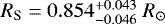 by Berger et al. (2018). While the effective temperature perfectly fits the HIRES value, the stellar radius is significantly smaller. It fits within the 1σ range of the value derived by the photodynamical analysis, and within the 2σ range the value derived with the stellar evolution models. The distance of Kepler-82 is determined to
  by Berger et al. (2018).
The discrepancy between stellar parameters derived by Gaia and by the combination of the photodynamical analysis and spectroscopic parameters could be a hint of another star that contaminates the light of Kepler-82. Inspecting a small region around Kepler-82 revealed a star about two magnitudes fainter at 10 arcsec distance. This distance is large enough so that the Kepler lightcurve should not be contaminated by this star. In the unlikely case of contamination, the radii of the planets would be underestimated by ten percent in maximum. That would make Kepler-82c to be an even more puffed-up exoplanet in the Neptune-like regime. The stellar radius and hence the density should not be affected by the light of a second star, as it is dependent upon the transit duration which is not changed. This agrees well with the fact that the photodynamical determined stellar radius matches the Gaia radius within its errorbars. Itshould be noted that the largest discrepancy is between the Gaia and the spectroscopic measurement, whereas the photodynamical one is in between. A further research of this deviance is beyond the scope of this paper.
 |
Fig. 6 Mass-radius diagram for known planets with masses up to 20 M⊕. In yellow are the planets with mass measurements obtained by RVs and in green the planets with mass measurements obtained from TTVs. The data are given by The Extrasolar Planets Encyclopaedia. Our results are shown in red (Kepler-82b) and in blue (Kepler-82c). For comparison also the values of Uranus and Neptune are shown, the Neptune-like planet pair of our solar system. |
6 Conclusions
In this workthe first dynamical analysis of the Kepler-82 system was carried out, resulting in the discovery of a fifth planet. The signal of this planet is found in the TTVs of Kepler-82c. In addition to the sinusoidal behaviour due to the interaction with Kepler-82b being near the 2:1 resonance, the TTVs show the so called chopping signal manifesting in a jump every three consecutive transits. After optimising a 2-planet photodynamical model near the 2:1 resonance to the Kepler long- and short-cadence data, we analysed the data with two different 3-planet system models. The systems differ in the ratio of the distance of the outermost fifth planet to Kepler-82c, either a 6:2:1 or a 3:2:1 near-resonant system were possible. The first evidence that the 3:2:1 resonance system model was the correct assumption was provided by the  , which is a little better than the one from analysing with the 6:2:1 resonance model. The 3:2:1 resonance model is also more favourable considering the mass of planet f is of the same order as planets b and c. This system model better fits into the “peas in a pod” architecture of most systems found by Kepler (Weiss et al. 2018). This is emphasised by the light curves collected in the framework of KOINet. The three new transit observations prefer the 3:2:1 resonance model and in addition a light curve including no transit measurement was taken during the time where a transit was predicted by the 6:2:1 resonance model. Additionally, the avoidance of inclinations that lead to transits by the third planet in near 3:2 resonance fits very well with the observations. Finally, with the periods of the planets in the 3:2:1 resonance system, except for two of them the frequencies in the TTVs of Kepler-82b/c detected by Ofir et al. (2018) can be explained by the super and the chopping frequencies. The most important point here is that Ofir et al. (2018) noticed a significant offset in the highest amplitude frequency of the TTVs of Kepler-82c from the near 2:1 mean motion resonance frequency. This peak is explained by the super frequency of the near 3:2 resonance of Kepler-82f and Kepler-82c. We conclude with announcing the detection of a fifth planet positioned in near 3:2 resonance to Kepler-82c. After the recent discovery of Kepler-411e(Sun et al. 2019), Kepler-82f is the second non-transiting planet detected via the TTVs of two other planets.
Determining the correct system architecture is important for modelling the right planet compositions. These highly depend on the assumed system architecture. The 2-planet model with significantly higher  supposes a density ratio between planet b and c of about ~14, whereas in the 3:2:1 resonance model especially the mass of Kepler-82b drops by about an order of magnitude resulting in a much more common (and reasonable) density ratio of ~ 2.
Acknowledgements
We acknowledge funding from the German Research Foundation (DFG) through grant DR 281/30-1. This work made use of PyAstronomy. This research has made use of the NASA Exoplanet Archive, which is operated by the California Institute of Technology, under contract with the National Aeronautics and Space Administration under the Exoplanet Exploration Program. C.v.E. acknowledges funding for the Stellar Astrophysics Centre, provided by The Danish National Research Foundation (Grant DNRF106), and support from the European Social Fund via the Lithuanian Science Council grant No. 09.3.3-LMT-K-712-01-0103. E.H. and I.R. acknowledge support from the Spanish Ministry of Economy and Competitiveness (MINECO) and the Fondo Europeo de Desarrollo Regional (FEDER) through grant ESP2016-80435-C2-1-R, as well as the support of the Generalitat de Catalunya/CERCA program. EA is supported by the United States National Science Foundation grant 1615315. Based on observations obtained with the Apache Point Observatory 3.5-m telescope, which is owned and operated by the Astrophysical Research Consortium. We acknowledge support from the Research Council of Norway (grant 188910) to finance service observing at the NOT. SW acknowledges support for International Team 265 (“Magnetic Activity of M-type Dwarf Stars and the Influence on Habitable Extra-solar Planets”) funded by the International Space Science Institute (ISSI) in Bern, Switzerland, and by the Research Council of Norway through its Centres of Excellence scheme, project number 262622.
Appendix A Additional plots and tables
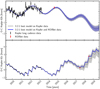 |
Fig. A.1 O–C diagram of Kepler-82b at the top and Kepler-82c at the bottom with transit times from modelling the transits individually. The black points refer to the transit data from the Kepler telescope. The red points are the individual transit times from the new KOINet observations. The grey area indicates the 68.3% confidence interval of the 3:2:1 resonance model fitted to the Kepler long- and short-cadence data only, the grey line is the best χ2 solution. The blue area indicates the same model solution applied to Kepler and KOINet data respectively. |
 |
Fig. A.2 Configurations of the Kepler-82 system. With the star in grey on the left side and the observer on the right side this shows the two different configurations: b in violet has the same position in both, c and f in red shows configuration I and in blueconfiguration II. The grey area indicates the region of impact parameters below one. The distances are true to scale with the stellar radius. Additionally, the two inner planets are plotted in green, the data are taken from the NASA Exoplanet Archive. They are plotted on both sides because we did not include them in the photodynamical analysis andhence we do not know how they behave in the two configurations. |
 |
Fig. A.3 Correlation plot of all fit parameters from modelling the 3:2:1 resonance model to Kepler long- and short-cadence and KOINet data. |
Ephemerides E and transit time predictions in BJD-2 400 000.0 from modelling Kepler and KOINet data for the next 15 yr.
Stellar and planetary parameters from the photodynamical modelling of the 2:1 resonance solution on Kepler long- and short-cadence data, the 6:2:1 resonance solution on Kepler data, the 3:2:1 resonance solution on Kepler data, the 3:2:1 resonance solution on Kepler data and the three KOINet transit light curves, and some corrections from investigating stellar evolution models in Sect. 5.4.
References
- Agol, E., & Fabrycky, D. C. 2018, Transit-Timing and Duration Variations for the Discovery and Characterization of Exoplanets (Berlin: Springer), 7 [Google Scholar]
- Almenara, J. M., Díaz, R. F., Mardling, R., et al. 2015, MNRAS, 453, 2644 [NASA ADS] [CrossRef] [Google Scholar]
- Almenara, J. M., Díaz, R. F., Bonfils, X., & Udry, S. 2016, A&A, 595, L5 [NASA ADS] [CrossRef] [EDP Sciences] [Google Scholar]
- Almenara, J. M., Díaz, R. F., Dorn, C., Bonfils, X., & Udry, S. 2018a, MNRAS, 478, 460 [NASA ADS] [CrossRef] [Google Scholar]
- Almenara, J. M., Díaz, R. F., Hébrard, G., et al. 2018b, A&A, 615, A90 [NASA ADS] [CrossRef] [EDP Sciences] [Google Scholar]
- Barnes, S. A. 2007, ApJ, 669, 1167 [NASA ADS] [CrossRef] [Google Scholar]
- Barnes, S. A. 2009, in The Ages of Stars, eds. E. E. Mamajek, D. R. Soderblom, & R. F. G. Wyse, IAU Symp., 258, 345 [NASA ADS] [Google Scholar]
- Barros, S. C. C., Almenara, J. M., Demangeon, O., et al. 2015, MNRAS, 454, 4267 [NASA ADS] [CrossRef] [Google Scholar]
- Berger, T. A., Huber, D., Gaidos, E., & van Saders, J. L. 2018, ApJ, 866, 99 [NASA ADS] [CrossRef] [Google Scholar]
- Borucki, W. J., Koch, D. G., Batalha, N., et al. 2012, ApJ, 745, 120 [NASA ADS] [CrossRef] [Google Scholar]
- Bovaird, T., Lineweaver, C. H., & Jacobsen, S. K. 2015, MNRAS, 448, 3608 [NASA ADS] [CrossRef] [Google Scholar]
- Chambers, J. E. 1999, MNRAS, 304, 793 [NASA ADS] [CrossRef] [MathSciNet] [Google Scholar]
- Choi, J., Dotter, A., Conroy, C., et al. 2016, ApJ, 823, 102 [NASA ADS] [CrossRef] [Google Scholar]
- Claret, A., & Bloemen, S. 2011, A&A, 529, A75 [NASA ADS] [CrossRef] [EDP Sciences] [Google Scholar]
- Dotter, A. 2016, ApJS, 222, 8 [NASA ADS] [CrossRef] [Google Scholar]
- Doyle, L. R., Carter, J. A., Fabrycky, D. C., et al. 2011, Science, 333, 1602 [NASA ADS] [CrossRef] [MathSciNet] [PubMed] [Google Scholar]
- Everett, M. E., Howell, S. B., & Kinemuchi, K. 2012, PASP, 124, 316 [NASA ADS] [CrossRef] [Google Scholar]
- Fabrycky, D. C., Ford, E. B., Steffen, J. H., et al. 2012, ApJ, 750, 114 [NASA ADS] [CrossRef] [Google Scholar]
- Foreman-Mackey, D., Hogg, D. W., Lang, D., & Goodman, J. 2013, PASP, 125, 306 [CrossRef] [Google Scholar]
- Freudenthal, J., von Essen, C., Dreizler, S., et al. 2018, A&A, 618, A41 [NASA ADS] [CrossRef] [EDP Sciences] [Google Scholar]
- Gaia Collaboration (Prusti, T., et al.) 2016, A&A, 595, A1 [NASA ADS] [CrossRef] [EDP Sciences] [Google Scholar]
- Gaia Collaboration (Brown, A. G. A., et al.) 2018, A&A, 616, A1 [NASA ADS] [CrossRef] [EDP Sciences] [Google Scholar]
- Goodman, J., & Weare, J. 2010, Comm. App. Math. Comp. Sci., 5, 65 [Google Scholar]
- Hadden, S., & Lithwick, Y. 2014, ApJ, 787, 80 [Google Scholar]
- Holczer, T., Mazeh, T., Nachmani, G., et al. 2016, ApJS, 225, 9 [NASA ADS] [CrossRef] [Google Scholar]
- Johnson, J. A., Petigura, E. A., Fulton, B. J., et al. 2017, VizieR Online Data Catalog: J/AJ/154/108 [Google Scholar]
- Kidder, L. E. 1995, Phys. Rev. D, 52, 821 [NASA ADS] [CrossRef] [Google Scholar]
- Kipping, D. M. 2010, MNRAS, 408, 1758 [NASA ADS] [CrossRef] [Google Scholar]
- Kjeldsen, H., & Frandsen, S. 1992, PASP, 104, 413 [NASA ADS] [CrossRef] [Google Scholar]
- Lomb, N. R. 1976, Ap&SS, 39, 447 [NASA ADS] [CrossRef] [Google Scholar]
- Mandel, K., & Agol, E. 2002, ApJ, 580, L171 [NASA ADS] [CrossRef] [Google Scholar]
- Mazeh, T., Nachmani, G., Holczer, T., et al. 2013, ApJS, 208, 16 [NASA ADS] [CrossRef] [Google Scholar]
- Morbidelli, A. 2002, Modern Celestial Mechanics: Aspects of Solar System dynamics (London: Taylor & Francis) [Google Scholar]
- Ofir, A., Xie, J.-W., Jiang, C.-F., Sari, R., & Aharonson, O. 2018, ApJS, 234, 9 [NASA ADS] [CrossRef] [Google Scholar]
- Paxton, B., Bildsten, L., Dotter, A., et al. 2011, ApJS, 192, 3 [Google Scholar]
- Paxton, B., Cantiello, M., Arras, P., et al. 2013, ApJS, 208, 4 [NASA ADS] [CrossRef] [Google Scholar]
- Paxton, B., Marchant, P., Schwab, J., et al. 2015, ApJS, 220, 15 [Google Scholar]
- Petigura, E. A., Howard, A. W., Marcy, G. W., et al. 2017, AJ, 154, 107 [NASA ADS] [CrossRef] [Google Scholar]
- Rowe, J. F., Bryson, S. T., Marcy, G. W., et al. 2014, ApJ, 784, 45 [NASA ADS] [CrossRef] [Google Scholar]
- Scargle, J. D. 1982, ApJ, 263, 835 [NASA ADS] [CrossRef] [Google Scholar]
- Southworth, J., Hinse, T. C., Jørgensen, U. G., et al. 2009, MNRAS, 396, 1023 [NASA ADS] [CrossRef] [Google Scholar]
- Steele, I. A., Smith, R. J., Rees, P. C., et al. 2004, in Ground-based Telescopes, ed. J. M. Oschmann, Jr., Proc. SPIE, 5489, 679 [CrossRef] [Google Scholar]
- Steffen, J. H., Fabrycky, D. C., Agol, E., et al. 2013, MNRAS, 428, 1077 [NASA ADS] [CrossRef] [Google Scholar]
- Sun, L., Ioannidis, P., Gu, S., et al. 2019, A&A, 624, A15 [NASA ADS] [CrossRef] [EDP Sciences] [Google Scholar]
- von Essen, C., Schröter, S., Agol, E., & Schmitt, J. H. M. M. 2013, A&A, 555, A92 [NASA ADS] [CrossRef] [EDP Sciences] [Google Scholar]
- von Essen, C., Ofir, A., Dreizler, S., et al. 2018, A&A, 615, A79 [NASA ADS] [CrossRef] [EDP Sciences] [Google Scholar]
- Weiss, L. M., Marcy, G. W., Petigura, E. A., et al. 2018, AJ, 155, 48 [NASA ADS] [CrossRef] [Google Scholar]
- Xie, J.-W. 2013, ApJS, 208, 22 [NASA ADS] [CrossRef] [Google Scholar]
- Zechmeister, M., & Kürster, M. 2009, A&A, 496, 577 [NASA ADS] [CrossRef] [EDP Sciences] [Google Scholar]
All Tables
Characteristics of collected ground-based transit light curves of Kepler-82b/c, collected through KOINet.
Planetary and Stellar parameters from photodynamical analysis of the 3:2:1 resonance model on Kepler data and the three KOINet transit light curves.
Properties of the optimisation of different models paired with different data sets.
Comparison between TTV inducing frequencies calculated from periods of the system solution to measured TTV frequencies by Ofir et al. (2018).
Ephemerides E and transit time predictions in BJD-2 400 000.0 from modelling Kepler and KOINet data for the next 15 yr.
Stellar and planetary parameters from the photodynamical modelling of the 2:1 resonance solution on Kepler long- and short-cadence data, the 6:2:1 resonance solution on Kepler data, the 3:2:1 resonance solution on Kepler data, the 3:2:1 resonance solution on Kepler data and the three KOINet transit light curves, and some corrections from investigating stellar evolution models in Sect. 5.4.
All Figures
|
Fig. 1 O–C diagrams of Kepler-82b at the top and Kepler-82c at the bottom with transit times from modelling the transits individually. The black points refer to the transit data from the Kepler telescope. The red points are the individual transit times from the new KOINet observations (plotted in Fig. 2). The violet lines show observed epochs but with non-detections of transit. The green area indicates the 99.7% (light) and the 68.3% (dark) confidence interval of the 6:2:1 resonance model optimised on Kepler long- and short-cadence data only, derived from 1000 randomly chosen models out of the MCMC posterior distribution; the green line is the median. The blue areas indicate the 3:2:1 resonance model solution. The grey areas present the 2:1 resonance model. |
| In the text | |
|
Fig. 2 KOINet transit light curves of Kepler-82. The three transit light curves (black) are overplotted with 1000 random models of the 3:2:1 resonance optimised using Kepler long- and short-cadence data (red) and including these KOINet observations(blue). |
| In the text | |
|
Fig. 3 Configurations of the Kepler-82 system. With the star in grey on the left side and the observer on the right side this shows the two different configurations: b in violet has the same position in both, c and f in red shows configuration I and in blue configuration II. The grey area indicates the region of impact parameters below one. The distances are not true to scale with the stellar radius, therefore a few inclination values are indicated as dashed grey lines. A similar plot with true scales can be found in Fig. A.2. |
| In the text | |
|
Fig. 4 Mass-age diagram of Kepler-82 from MESA stellar evolution models (MIST). The black star and the red, orange, and grey dots correspond to the best matching value and the 1σ, 2σ, and 3σ areas derived from results on the density of the whole set photodynamical modelling and from the literature values of the effective temperature, the surface gravity, and the metallicity by Petigura et al. (2017). The gyrochronologic age is indicated in green by a solid line and its 1σ range as dashed lines. |
| In the text | |
|
Fig. 5 Radius-age diagram of Kepler-82 from MESA stellar evolution models (MIST). The black star and the red, orange, and grey dots correspond to the best matching value and the 1σ, 2σ, and 3σ areas derived from results on the density of the whole data set photodynamical modelling and from the literature values of the effective temperature, the surface gravity, and the metallicity by Petigura et al. (2017). The gyrochronologic age is indicated in green by a solid line and its 1σ range as dashed lines. |
| In the text | |
|
Fig. 6 Mass-radius diagram for known planets with masses up to 20 M⊕. In yellow are the planets with mass measurements obtained by RVs and in green the planets with mass measurements obtained from TTVs. The data are given by The Extrasolar Planets Encyclopaedia. Our results are shown in red (Kepler-82b) and in blue (Kepler-82c). For comparison also the values of Uranus and Neptune are shown, the Neptune-like planet pair of our solar system. |
| In the text | |
|
Fig. A.1 O–C diagram of Kepler-82b at the top and Kepler-82c at the bottom with transit times from modelling the transits individually. The black points refer to the transit data from the Kepler telescope. The red points are the individual transit times from the new KOINet observations. The grey area indicates the 68.3% confidence interval of the 3:2:1 resonance model fitted to the Kepler long- and short-cadence data only, the grey line is the best χ2 solution. The blue area indicates the same model solution applied to Kepler and KOINet data respectively. |
| In the text | |
|
Fig. A.2 Configurations of the Kepler-82 system. With the star in grey on the left side and the observer on the right side this shows the two different configurations: b in violet has the same position in both, c and f in red shows configuration I and in blueconfiguration II. The grey area indicates the region of impact parameters below one. The distances are true to scale with the stellar radius. Additionally, the two inner planets are plotted in green, the data are taken from the NASA Exoplanet Archive. They are plotted on both sides because we did not include them in the photodynamical analysis andhence we do not know how they behave in the two configurations. |
| In the text | |
|
Fig. A.3 Correlation plot of all fit parameters from modelling the 3:2:1 resonance model to Kepler long- and short-cadence and KOINet data. |
| In the text | |
Current usage metrics show cumulative count of Article Views (full-text article views including HTML views, PDF and ePub downloads, according to the available data) and Abstracts Views on Vision4Press platform.
Data correspond to usage on the plateform after 2015. The current usage metrics is available 48-96 hours after online publication and is updated daily on week days.
Initial download of the metrics may take a while.