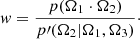
| Issue |
A&A
Volume 628, August 2019
|
|
|---|---|---|
| Article Number | A105 | |
| Number of page(s) | 8 | |
| Section | Numerical methods and codes | |
| DOI | https://doi.org/10.1051/0004-6361/201935751 | |
| Published online | 13 August 2019 | |
A guided Monte Carlo radiative transfer method using mixture importance sampling
School of Mathematical and Physical Sciences, Dalian University of Technology, Panjin, PR China
e-mail: This email address is being protected from spambots. You need JavaScript enabled to view it.
Received:
22
April
2019
Accepted:
15
July
2019
Abstract
In order to investigate the source of uncertainties for the Monte Carlo radiative transfer method, a path space formulation is proposed which expresses the integral form of the radiative transfer equation. It has been determined that some of the uncertainties depend on the sampling of photon propagation directions. To reduce this kind of uncertainty, we propose a guided Monte Carlo (GMC) method based on a direction mixture importance sampling strategy for simulating radiative transfer in a scattering medium. We validated the GMC method by implementing it in a backward Monte Carlo radiative transfer (BMCRT) code for the plane-parallel medium. Similar to the usual BMCRT method, the solution is determined by tracing photons from the detector towards the radiation source in the backward GMC method. Through test examples, we demonstrate the validity of the direction mixture importance sampling strategy and the GMC method.
Key words: radiative transfer
© ESO 2019
1. Introduction
Scattering and absorption greatly impact radiation transport in the planetary atmosphere (Liou 2002) and interstellar medium (Draine 2011), which is the key for understanding the physical properties of the medium and radiation source. Spectroscopic inference in astrophysics relies on knowledge of the transport properties of the medium. It is important to note that the radiative transfer equation (RTE) does not have analytic solutions, so numerical methods have to be applied to solve equations. Among these numerical methods, the Monte Carlo method (MCM) is an exceptional one, which is widely used in nearly all quantitative fields, such as mathematical and physical sciences, computer science, engineering, and quantitative economics et. al. In the context of astrophysics, the Monte Carlo radiative transfer (MCRT) method (Whitney 2011; Steinacker et al. 2013) can find solutions for RTEs in a mathematically rigorous way and also provide an intuitive interpretation about the stochastic nature of the radiation transport process. Since MCMs solve the integration problem by generating realisations of random variables from specific distributions, the convergence rate does not depend on the number of dimensions. This, in particular, makes it an attractive method for evaluating integrals in high dimensions. Decades after its birth, MCRT has proven to be a successful tool for studying radiative transfer in inhomogeneous or heterogeneous mediums with complex geometries (Pharr & Humphreys 2010).
The main disadvantage of MCMs is their slow convergence rate. For the Monte Carlo radiative transfer method, it is often the case that millions of “photons” must be traced to compute the radiance, which is quite expensive in time (here, we refer to photon as a phenomenological object and not as the particle in quantum physics). Hence, several variance reduction and acceleration techniques have been proposed. Most of these methods can be classified, to some extent, as importance sampling techniques (biasing) that trace photons. An example of this type of method is forced collision (Mattila 1970), which improves the efficiency of MCRT in an optically thin medium. Juvela (2005) proposed an importance sampling strategy for propagation directions and for weights of photons split into equal parts. In the context of biomedical applications, Lima et al. (2011) developed a biased scattering direction importance sampling method to speed up Monte Carlo simulations of photon transport in tissue. Recently, Baes et al. (2016) and Camps & Baes (2018) proposed the use of a composite biasing technique, which is mixture with importance sampling (Hesterberg 1995), and applied it to various sampling processes in MCRT.
In this paper, we present a guided Monte Carlo radiative transfer method. In Sect. 2, we show how the integral form of RTE can be related to path space formulation. This formulation will be used in analysing the source of uncertainty and inspire new sampling methods for reducing the variance in MCRT. In Sect. 3, we propose the idea of bidirectional conditional scattering phase function and its sampling methods. Mixture importance sampling and its use in MCRT are introduced thereafter. In Sect. 4, we demonstrate the validity of mixture importance sampling and compare the guided Monte Carlo method with classical Monte Carlo method. In Sect. 5, we make a summary of the main conclusions.
2. Model
It is interesting to note that is is difficult to solve the radiative transfer in a plane-parallel atmosphere illuminated by solar radiation at a specific wavelength. The radiance in a specific volume changes due to light scattering and absorption processes. Therefore, our goal is to solve a time independent radiative transfer equation without emission sources in the volume or on the boundary,
 (1)
(1)
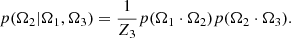
where L represents the radiance, r is a position vector, Ω and Ω′ are unit direction vectors, βe and βs are the extinction and the scattering coefficients respectively, and p(Ω, Ω′, r) is the scattering phase function.
When we solved RTE with the Monte Carlo method, the radiance recorded by the detector was expressed as the sum of the successive order of scattering series:
 (2)
(2)
where Lj are contributions from photons scattered by exactly j times after entering the volume. Each component of the scattering series can be expressed as an integral,
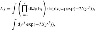 (3)
(3)
where γj is the photon path with the probability measure dγj, τi is optical depth, and ℋ is a function of the photon path γj,
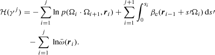 (4)
(4)
Here,  is the single scattering albedo. This is actually a negative log-likelihood function, which is quite similar to the energy function in polymer statistical physics and has been used for solving radiative transfer problems (Frederickx & Dutré 2017). It is noted that similar path space integral techniques (Pauly et al. 2000; Premože et al. 2003; Jakob 2016) have been widely used in computer graphics for physically based rendering.
3. Method
3.1. Importance sampling
Depending on the starting position of tracing for the source or detector, the MCRT methods are usually divided into forward and backward (FMCRT and BMCRT; García Munoz & Mills 2015) categories. We note that FMCRT traces photons from sources and is efficient if the limited source area or the range of emission directions are considered. Conversely, the BMCRT method traces photons in the opposite way and is efficient if the limited detection area or the range of detection directions are taken into account. Both FMCRT and BMCRT estimate radiance using the importance sampling strategy, which is expressed as an integral as follows:
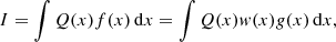 (5)
(5)
where Q(x) is a function, f(x) and g(x) are probability density functions, and w(x)=f(x)/g(x) is the likelihood ratio. Hence, the importance sampling estimate of I (Robert & Casella 2010) is
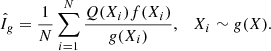 (6)
(6)
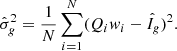
This estimate is unbiased with the variance 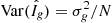 . And
. And  can be estimated as
 (7)
(7)
The performance of an importance sampling rule depends on the choice of g(x). In the classical BMCRT method, the photon path is traced from the detector with a local estimation scheme (Liou 2002) when each scattering event occurs. In the local estimation scheme, photons are scattered in the incident direction. This scheme is extremely efficient in mediums with small-sized particles (in comparison to photon wavelength) in which Rayleigh scattering or isotropic scattering are the most common. But for mediums with large-sized particles, whose scattering phase functions have strong forward peaks, this scheme may lead to fairly large variance in the computed radiance. More analyses will be given in the following.
We considered a simple toy model first in which the medium was assumed to be infinite, isotropic, homogeneous, and non-absorbing. We considered the angular distribution of photons after exact n scattering. In essence, our intention was to compute the integration of a joint scattering phase function given incoming and outgoing propagation directions Ω1 and Ωn:
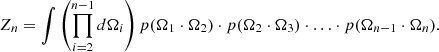 (8)
(8)
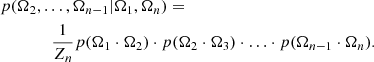
The most common approach is to generate samples from the conditional distribution f(x)=p(Ω2, …, Ωn − 1|Ω1) and then random (direction) scattering directions Ω2, …, Ωn − 1 are generated sequentially. This approach selects the initial fixed direction and successively samples scattering directions with the last scattering phase function term as Q(x)=p(Ωn − 1 ⋅ Ωn). That is, we sampled Ω2 from p(Ω2|Ω1)=p(Ω1 ⋅ Ω2) and then we conditionally sampled each successive propagation direction on the following previous directions:
 (9)
(9)
This sequential generation method is summarised in Algorithm 1.
1: for i in 2 : n − 1
2: Sample Ωi ∼ p(Ωi|Ωi−1,…, Ω1) = p(Ωi−1 ⋅ Ωi)
3: return Ωn−1
This method works well in nearly isotropic scattering cases. However, as we have stated above, values of a scattering phase function with a strongly forward peak vary over several orders, which leads to a fairly large variance. If the random samples are drawn from a distribution that is similar to the integrand, the variance will decrease as follows:
 (10)
(10)
Since Zn is a constant, each estimate is exactly the same and the variance will actually be zero. Of course, this is an extreme case and it is not necessary to use the Monte Carlo method. However, this indicates to us that both incoming and outgoing directions are important in sampling photon propagation directions.
3.2. Guided Monte Carlo (GMC) method and mixture importance sampling
The scattering phase function plays a fundamental role in determining behaviours of radiative transfer in a scattering medium. In this section, two types of what we refer to as bidirectional conditional scattering phase functions are proposed for simulating radiative transfer with a GMC method. A mixture importance sampling strategy with conditional scattering phase functions is also presented, which can reduce the variance of simulated spectroscopic quantities.
3.2.1. Conditional scattering phase function and Gibbs sampling
The first candidate for the bidirectional conditional scattering phase function is
 (11)
(11)
Consider the phase function proposed by Henyey & Greenstein (1941):
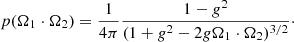 (12)
(12)
It is easy to obtain the normalisation constant, that is
 (13)
(13)
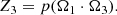
The method that best generates samples from conditional distributions is the Gibbs sampler. By introducing one auxiliary variable, the full conditional densities can all be sampled. See Robert & Casella (2010) for more discussions on auxiliary variables and the Gibbs sampler. The key objective of the Gibbs sampler is to choose a joint probability density from which one can easily sample the conditional densities. Here, the joint density function for the HG phase function can be written as
 (14)
(14)
where 𝕀(⋅) is the indicator function 1, if u < p(Ω1 ⋅ Ω2) and 0 elsewhere.
We started the Gibbs sampler by first sampling Ω2 from a few suitable density functions. We then sampled the full conditionals, in the usual way, that is done by updating the last direction in the conditional density with a new direction. Detailed steps are described in Algorithm 2.
1: Sample 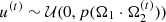
2: do
3: Ω2 ∼ p(Ω2 ⋅ Ω3)
4: while (p(Ω1 ⋅ Ω2 < u(t)
5: return 
To achieve the stationary distribution, the length of the “burn-in” period must be large enough. The random sequence generated by the Gibbs sampler is a dependent sequence with positive auto-correlation. Due to the dependance, the size of the samples that are simulated with a Markov chain need to be large enough. Therefore, we thinned the chain and retained every nth iteration. In the trace plot (as in Fig. 1) of the x-component of the scattering direction, direction samples that were generated from Markov chains were thinned so that every 5th (middle panel) and 10th (bottom panel) iteration were retained. Thinning can make computational time faster by reducing the sample size. It can also improve the randomness of samples. After running the chain, auto-correlation functions corresponding to above sample sequences are plotted in Fig. 2. Figure 3 shows trace plots of all three components of the scattering direction thinned by every 10th iteration. Furthermore, their auto-correlation functions are plotted in Fig. 4. Gibbs sampling of bidirectional conditional scattering phase functions is shown in Fig. 5.
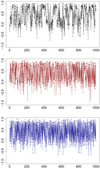 |
Fig. 1. Trace plots of x component of random directions corresponding to Markov chains before thinning (top panel) and after thinning with every 5th (middle panel) and 10th (bottom panel) iteration. The burn-in period is considered to be 100. |
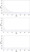 |
Fig. 2. Auto-correlation functions corresponding to Markov chains before thinning (top panel) and after thinning with every 5th (middle panel) and 10th (bottom panel) iteration. |
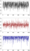 |
Fig. 3. Trace plots of three components of random directions corresponding to Markov chains after thinning with every 10th iteration. These panels (from top to bottom) represent the x-component, y-component, and z-component, respectively. The burn-in period is considered to be 100. |
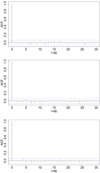 |
Fig. 4. Auto-correlation functions for three components corresponding to Markov chains after thinning with every10th iteration. These panels (from top to bottom) represent the x-component, y-component, and z-component, respectively. |
 |
Fig. 5. Spread of direction samples over unit sphere sampled from (left panel) joint HG scattering phase function and (right panel) mixture HG scattering phase function (q is set to 0.5). |
3.2.2. Mixture importance sampling
Sampling using Markov chains have substantial drawbacks since samples are dependent, which leads to slow convergence to the desired density function. In practice, thousands of samples might be discarded to obtain independent “random” samples. A long burn-in period is sometimes needed to make sure that the Markov Chain is stationary. Here, we propose to do the simulation by introducing a bidirectional conditional scattering phase function, which is defined as a mixture distribution,
 (15)
(15)
The above strategy is a specific form of the mixture importance sampling. In the mixture sampling strategy, we generated samples that were not from the original density p(x), but from a mixture density p′(x). After a sample is generated, the weight is updated by multiplying a factor of p(x)/p′(x). When mixture importance sampling is applied to direction sampling in MCRT, this leads to what we call the guided Monte Carlo method, (see Algorithm 3),
 (16)
(16)
Scattering direction samples from the HG mixture scattering phase function (q = 0.5) is shown in Fig. 5 (right panel). In the context of biomedical applications, Lima et al. (2011) proposed an important sampling strategy for scattering directions. In their work, a bias scattering phase function (equivalent to q = 0 in Eq. (15)) is used for a few specific regions, or layers, of the medium.
1: Sample w ← 1
2: for i in 1:n−1
3: Sample Ωi ∼ p′(Ωi|Ωi−1,Ωg) ▹ e.g. Ωg = Ωn
4: 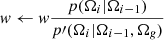
5: w ← wp(Ωn−1 ⋅ Ωn)
3.3. Sampling direction and free path length
It is important to note that MCRT are based on the sampling of random variables such as propagation direction, free path length, etc. Furthermore, the scattering direction follows the scattering phase function,
 (17)
(17)
where Ω and Ω′ are the incident and scattered directions, respectively. Obviously, Ω′ is the random variable. Also, the scattering phase function p(Ω ⋅ Ω′) describes the angular distribution of scattered photons, which can also be viewed as a conditional probability density function p(Ω′|Ω). Given the incident direction Ω. μ is the cosine of the angle θ between Ω and Ω′, ϕ is the azimuthal angle uniformly distributed over [0, 2π) with pϕ(ϕ)=1/2π.
There are many ways (Robert & Casella 2010) to generate random varieties of μ like the inverse cumulative distribution function (CDF) method. For example, the random variable X (μ or ϕ) can be generated by taking an inverse transform of a uniform random variable ξ on (0, 1) if its inverse CDF FX(x) exists as
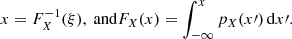 (18)
(18)
The example we consider here is radiative transfer in the planetary atmosphere. Therefore, if the photon travels downwards in the atmosphere, it may hit the ground and the unbiased distribution will be used. In this case, the photon can collide with either particles in the medium or the ground:
 (19)
(19)
If the photon travels upwards, the truncated exponential distribution is needed for sampling. Sampling from the truncated distribution means a collision process must occur before the photon escapes from the upper boundary. This sampling process introduces a bias which can be removed by rescaling the weight by the factor  . This factor is indeed the escaping probability that indicates that no collision or absorption has occurred within the follwing medium:
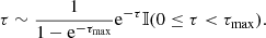 (20)
(20)
4. Results and discussions
To validate the GMC method, we compared its performance with the common sequential sampling method. In the first case, we used a simple integral that is the product of two HG phase functions with parameters g = 0.9 and g′=0.8, where
 (21)
(21)
The exact value of I is known. Table 1 gives simulation results for four sampling methods. In Table 1, the sample size, n = 104, is fixed and estimates of I and its standard deviation are given. In the GMC method, a mixture of HG phase function is used,
 (22)
(22)
Also, in the case using Gibbs sampling, the following joint scattering phase function is used:
 (23)
(23)
The angle between Ω1 and Ω3 is set to 60°, hence Ω1 ⋅ Ω3 = 0.5. This illustrates that the Gibbs sampler performs best in terms of sample variance, GMC with q = 0.5 has the second best performance, while the brute force method with a uniform sampling strategy is the least effective. Although the Gibbs sampler results in the lowest error, it takes more computational time since longer random sequences are needed to obtain the same size of independent samples.
In the GMC method, we applied a mixture importance sampling technique to sampling propagation directions in MCRT. Furthermore, this sampling method was implemented in a BMCRT code with plane-parallel geometry (Fig. 6). Figures 7a, 8a, and 9a compare the bootstrapped standard deviation of simulated radiance for a plane-parallel medium with optical depth τ = 1, 5, 10, respectively, using these two methods. The result shows that the values of estimated standard deviation for the GMC method are much smaller than those for the usual MC method over all viewing angles. Lengths of 95% bootstrapped confidence intervals of the estimated standard deviation are plotted in Figs. 7b, 8b, and 9b. As can be seen, the GMC radiative transfer method outperforms the usual backward Monte Carlo radiative transfer method over all viewing angles.
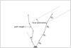 |
Fig. 6. Schematic representation of sample photon path generated by backward MC method. |
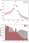 |
Fig. 7. q is set to 0.5, optical depth is 1.0. Top panel: estimated standard deviation of transmitted radiance calculated with the backward GMC method and classical backward MC method. Bottom panel: length of 95% bootstrapped confident intervals (CIs) for the estimated standard deviation. |
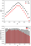 |
Fig. 8. q is set to 0.95, optical depth is 5.0. Top panel: estimated standard deviation of transmitted radiance calculated with the backward GMC method and classical backward MC method. Bottom panel: length of 95% bootstrapped confident intervals (CIs) for the estimated standard deviation. |
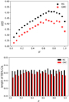 |
Fig. 9. q is set to 0.95, optical depth is 10.0. Top panel: estimated standard deviation of transmitted radiance calculated with the backward GMC method and classical backward MC method. Bottom panel: length of 95% bootstrapped confident intervals (CIs) for the estimated standard deviation. |
Figure 10a shows the estimated standard deviation for viewing angle (0) as a function of total optical depth. Also, we see that the GMC method can reduce the variance of simulated radiance for all of the optical depth over the range [1, 10]. The CPU time of these simulations is plotted in Fig. 10b. Both of them increase linearly as a function of optical depth, and simulations with the GMC method take about 50% more time than the usual backward MC method. And the result simulated with the MC method converges to the correct solution at a rate of 𝒪(N−1/2) (N is the number of samples). In other words, to reduce the error (estimated standard deviation) by half, four times as many samples can be used in the simulation. Therefore, the mixture importance sampling technique has more positive than negative aspects in regards to computational time.
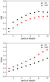 |
Fig. 10. Top panel: estimated standard deviation of transmitted radiance calculated with backward GMC method and classical backward MC method for single viewing angle μ = 1 with optical depths from 1 to 10. Bottom panel: simulation time as a function of optical depth using these two methods. |
Extension to more complex geometries or vector radiative transfer cases (García Munoz & Mills 2015) is easy and will be discussed in our further works. Also, our results support the applicability of GMCRT, especially for the optically thick medium. It should also be noted that GMC smoothes the underlying integrand in the integral formulation of the radiative transfer equation. Additionally, other sampling and variance reduction methods (Lux 1991) including path length stretching and Russian roulette can be used simultaneously with the GMCRT method. Path length stretching is an important sampling strategy that is widely used in Monte Carlo simulations of neutron transport problems. The idea of path length stretching is to replace exponential path length distribution with another modified distribution to generate samples using
 (24)
(24)
where α > 0 is the stretching parameter. Furthermore, Russian roulette is a variance reduction technique that can improve the estimate of Monte Carlo methods by increasing the likelihood of each sample. Russian roulette eliminates samples that make minor contributions to the estimate in a probabilistic manner. To apply the Russian roulette method, we needed to choose a threshold probability pr. With probability pr, the photon survives with its weight multiplied by 1/pr. With probability 1 − pr, the photon will be terminated with its weight reduced to zero.
In the classic MCRT method, random walk photons are traced from the beginning to the end. In the GMCRT method, the additional component of the mixture scattering phase function acts like a “force” dragging photons to the target direction. Generally speaking, the force is larger when q is smaller. In the above simulations, the GMC method was tested in a backward MCRT code for the homogeneous medium. Also, choices of the mixture ratio q were determined in an approximately optimal way. For the medium with higher optical depth, the average travelling distances of photons is larger. So a milder force (larger q) is needed for guiding the photons. But it should be noted that a bad choice of q will lead to bad simulation performance. Figure 11 compares estimated standard deviations of GMC simulated radiance for a plane-parallel medium with optical depth τ = 1 using q = 1.0, 0.5 and 0.0, where q = 1.0 corresponds to the original scattering phase function used in the classic MCRT method and q = 0.0 corresponds to the biased one proposed by Lima et al. (2011). Figure 11 clearly shows that the case of q = 0.0 performs rather badly, which means that the “force” is so large that simulated photon paths deviate too much from the important ones in this case. Since the GMC method is essentially a local method, it is quite flexible and can to be modified for applications. For example, it can be used for specific regions of the inhomogeneous medium by substituting the scattering phase function with a mixture biased one. An adaptive version of the GMC method is also possible by changing the mixture ratio q successively, according to the scattering order.
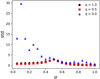 |
Fig. 11. Estimated standard deviation of transmitted radiance simulated with backward GMC method for q = 1.0, 0.5 and 0.0. |
5. Conclusions
In this paper, we proposed the idea that bidirectional conditional scattering phase functions show that they can be used for sampling directions in the MCRT method. We also provided a Gibbs sampler to simulate with a conditional scattering phase function. Based on this idea, we proposed a guided Monte Carlo method for simulating radiative transfer in a scattering medium. In our GMC method, mixture importance sampling was used to sample propagation directions with the mixture scattering phase function. Results show that the mixture importance sampling strategy gives much more efficient sampling and results in smaller variance of simulated quantities than the usual IS strategy. We find that variance can be reduced for all viewing angles in our simulation using a backward GMCRT method. This GMCRT method works well for mediums with large optical depth and is straightforward to implement in existing benchmark MCRT codes with little extra effort.
Acknowledgments
Part of this work was supported by the National Natural Science Foundation of China (NSFC) (Grant No. 41705010) and “The Fundamental Research Funds for the Central Universities” (DUT19RC(4)039).
References
- Baes, M., Gordon, K. D., Lunttila, T., et al. 2016, A&A, 590, A55 [NASA ADS] [CrossRef] [EDP Sciences] [Google Scholar]
- Camps, P., & Baes, M. 2018, ApJ, 861, 80 [NASA ADS] [CrossRef] [Google Scholar]
- Draine, B. T. 2011, Physics of the Interstellar and Intergalactic Medium (Princeton: Princeton University Press) [Google Scholar]
- Frederickx, R., & Dutré, P. 2017, ACM Trans. Graph., 36, 109 [CrossRef] [Google Scholar]
- García Munoz, A., & Mills, F. P. 2015, A&A, 573, A72 [NASA ADS] [CrossRef] [EDP Sciences] [Google Scholar]
- Henyey, L. C., & Greenstein, J. L. 1941, ApJ, 93, 70 [NASA ADS] [CrossRef] [Google Scholar]
- Hesterberg, T. 1995, Technometrics, 37, 185 [CrossRef] [Google Scholar]
- Jakob, W. 2016, in Monte Carlo and Quasi-Monte Carlo Methods, eds. R. Cools, & D. Nuyens (Cham: Springer International Publishing), 107 [CrossRef] [Google Scholar]
- Juvela, M. 2005, A&A, 440, 531 [NASA ADS] [CrossRef] [EDP Sciences] [Google Scholar]
- Lima, I. T., Kalra, A., & Sherif, S. S. 2011, Opt. Express, 2, 1069 [CrossRef] [Google Scholar]
- Liou, K.-N. 2002, An Introduction to Atmospheric Radiation, 2nd edn. (New York: Academic Press) [Google Scholar]
- Lux, I. 1991, Monte Carlo Particle Transport Methods: Neutron and Photon Calculations (New York: CRC Press) [Google Scholar]
- Mattila, K. 1970, A&A, 8, 273 [NASA ADS] [Google Scholar]
- Pauly, M., Kollig, T., & Keller, A. 2000, Proceedings of the Eurographics Workshop on Rendering Techniques 2000 (London (UK: Springer-Verlag)), 11 [CrossRef] [Google Scholar]
- Pharr, M., & Humphreys, G. 2010, Physically Based Rendering: From Theory to Implementation (Elsevier) [Google Scholar]
- Premože, S., Ashikhmin, M., & Shirley, P. 2003, Proceedings of the 14th Eurographics Workshop on Rendering, EGRW ’03 (Switzerland: Eurographics Association), 52 [Google Scholar]
- Robert, C. P., & Casella, G. 2010, Monte Carlo Statistical Methods (Berlin, Heidelberg: Springer) [Google Scholar]
- Steinacker, J., Baes, M., & Gordon, K. D. 2013, ARA&A, 51, 63 [NASA ADS] [CrossRef] [Google Scholar]
- Whitney, B. A. 2011, Bull. Astron. Soc. India, 39, 101 [NASA ADS] [Google Scholar]
All Tables
All Figures
|
Fig. 1. Trace plots of x component of random directions corresponding to Markov chains before thinning (top panel) and after thinning with every 5th (middle panel) and 10th (bottom panel) iteration. The burn-in period is considered to be 100. |
| In the text | |
|
Fig. 2. Auto-correlation functions corresponding to Markov chains before thinning (top panel) and after thinning with every 5th (middle panel) and 10th (bottom panel) iteration. |
| In the text | |
|
Fig. 3. Trace plots of three components of random directions corresponding to Markov chains after thinning with every 10th iteration. These panels (from top to bottom) represent the x-component, y-component, and z-component, respectively. The burn-in period is considered to be 100. |
| In the text | |
|
Fig. 4. Auto-correlation functions for three components corresponding to Markov chains after thinning with every10th iteration. These panels (from top to bottom) represent the x-component, y-component, and z-component, respectively. |
| In the text | |
|
Fig. 5. Spread of direction samples over unit sphere sampled from (left panel) joint HG scattering phase function and (right panel) mixture HG scattering phase function (q is set to 0.5). |
| In the text | |
|
Fig. 6. Schematic representation of sample photon path generated by backward MC method. |
| In the text | |
|
Fig. 7. q is set to 0.5, optical depth is 1.0. Top panel: estimated standard deviation of transmitted radiance calculated with the backward GMC method and classical backward MC method. Bottom panel: length of 95% bootstrapped confident intervals (CIs) for the estimated standard deviation. |
| In the text | |
|
Fig. 8. q is set to 0.95, optical depth is 5.0. Top panel: estimated standard deviation of transmitted radiance calculated with the backward GMC method and classical backward MC method. Bottom panel: length of 95% bootstrapped confident intervals (CIs) for the estimated standard deviation. |
| In the text | |
|
Fig. 9. q is set to 0.95, optical depth is 10.0. Top panel: estimated standard deviation of transmitted radiance calculated with the backward GMC method and classical backward MC method. Bottom panel: length of 95% bootstrapped confident intervals (CIs) for the estimated standard deviation. |
| In the text | |
|
Fig. 10. Top panel: estimated standard deviation of transmitted radiance calculated with backward GMC method and classical backward MC method for single viewing angle μ = 1 with optical depths from 1 to 10. Bottom panel: simulation time as a function of optical depth using these two methods. |
| In the text | |
|
Fig. 11. Estimated standard deviation of transmitted radiance simulated with backward GMC method for q = 1.0, 0.5 and 0.0. |
| In the text | |
Current usage metrics show cumulative count of Article Views (full-text article views including HTML views, PDF and ePub downloads, according to the available data) and Abstracts Views on Vision4Press platform.
Data correspond to usage on the plateform after 2015. The current usage metrics is available 48-96 hours after online publication and is updated daily on week days.
Initial download of the metrics may take a while.