| Issue |
A&A
Volume 627, July 2019
|
|
|---|---|---|
| Article Number | A153 | |
| Number of page(s) | 14 | |
| Section | Stellar structure and evolution | |
| DOI | https://doi.org/10.1051/0004-6361/201935516 | |
| Published online | 16 July 2019 | |
Absolute dimensions of the low-mass eclipsing binary system NSVS 10653195⋆
1
Astrophysics Department, Universidad de La Laguna, 38205 La Laguna, Tenerife, Spain
2
Centro de Estudios de Física del Cosmos de Aragón, Plaza San Juan 1, 44001 Teruel, Spain
e-mail: This email address is being protected from spambots. You need JavaScript enabled to view it.
3
Instituto de Astrofísica de Canarias, 38200 La Laguna, Tenerife, Spain
4
Harvard-Smithsonian Center for Astrophysics, 60 Garden Street, Cambridge, MA 02138, USA
5
NASA AMES Research Center, Moffet Field, CA, USA
Received:
20
March
2019
Accepted:
5
June
2019
Abstract
Context. Low-mass stars in eclipsing binary systems show radii larger and effective temperatures lower than theoretical stellar models predict for isolated stars with the same masses. Eclipsing binaries with low-mass components are hard to find due to their low luminosity. As a consequence, the analysis of the known low-mass eclipsing systems is key to understand this behavior.
Aims. We aim to investigate the mass–radius relation for low-mass stars and the cause of the deviation of the observed radii in low-mass detached eclipsing binary stars (LMDEB) from theoretical stellar models.
Methods. We developed a physical model of the LMDEB system NSVS 10653195 to accurately measure the masses and radii of the components. We obtained several high-resolution spectra in order to fit a spectroscopic orbit. Standardized absolute photometry was obtained to measure reliable color indices and to measure the mean Teff of the system in out-of-eclipse phases. We observed and analyzed optical VRI and infrared JK band differential light-curves which were fitted using PHOEBE. A Markov chain Monte-Carlo (MCMC) simulation near the solution found provides robust uncertainties for the fitted parameters.
Results. NSVS 10653195 is a detached eclipsing binary composed of two similar stars with masses of M1 = 0.6402 ± 0.0052 M⊙ and M2 = 0.6511 ± 0.0052 M⊙ and radii of R1 = 0.687+0.017−0.024 R⊙ and R2 = 0.672+0.018−0.022 R⊙. Spectral types were estimated to be K6V and K7V. These stars rotate in a circular orbit with an orbital inclination of i = 86.22 ± 0.61 degrees and a period of P = 0.5607222(2) d. The distance to the system is estimated to be d = 135.2+7.6−7.9 pc, in excellent agreement with the value from Gaia. If solar metallicity were assumed, the age of the system would be older than log (age) ∼ 8 based on the Mbol–log Teff diagram.
Conclusions. NSVS 10653195 is composed of two oversized and active K stars. While their radii is above model predictions their Teff are in better agreement with models.
Key words: stars: fundamental parameters / stars: low-mass / binaries: eclipsing / binaries: spectroscopic / stars: individual: NSVS 10653195
Full Tables 1–3 and 7 are only available at the CDS via anonymous ftp to cdsarc.u-strasbg.fr (130.79.128.5) or via http://cdsarc.u-strasbg.fr/viz-bin/qcat?J/A+A/627/A153
© ESO 2019
1. Introduction
Eclipsing binary stars are currently the most powerful tool to simultaneously measure the radii and masses of stars. By observing a photometric light curve (LC) and the radial velocity (RV) curves of the two components of the binary system it is possible to measure their masses and radii with precisions of a few percent, depending on the quality of the observational data. In recent years these techniques have also lead to the characterization of more than 3900 exoplanets around stars other than the Sun (see online databases12 for updated lists).
Stars in the upper main sequence are intrinsically luminous and can be observed at great distance in our Galaxy and even in other nearby galaxies (see, e.g. Ribas et al. 2005; Pietrzyński et al. 2013; Lee et al. 2014). As a result, applying these techniques to the upper main sequence stars provided a great number of stellar parameters and distances in that range of masses (see Torres et al. 2010, for a list of well measured systems). But the lower main sequence is a different issue, in particular the so-called low-mass stars, those with masses below 1 M⊙ and spectral types K and M. These stars are intrinsically faint and until a decade ago only half a dozen low-mass detached eclipsing binary systems (hereafter LMDEB) in the solar neighborhood were known, all of them with short periods (≲1 d or less). To make things worse, the low-mass stars are also affected by chromospheric and coronal activity caused by strong magnetic fields, dark and bright spots, flares, and plages. This activity can be observed as flares and modulation of the LCs at the out-of-eclipse orbital phases, X-ray emission, and emission spectral lines – usually CaII H and K or hydrogen lines (e.g., Hα). These features are difficult to model and add additional uncertainties to the physical parameters.
The data provided by the last generation of photometric surveys have improved this situation. Millions of LCs have thus far been provided by variable star and transient photometric databases like the North Sky Variability Survey (NSVS, Woźniak et al. 2004), or the All-Sky Automated Survey (ASAS, Pojmanski 1997), to name only two, databases devoted to searching for exoplanet transits from Earth, for example Wide Angle Search for Planets (WASP, Pollacco et al. 2006), Hungarian Automated Telescope (HAT, Bakos et al. 2004) and others, as well as databases devoted to searching for exoplanet transits from space, such as COnvection, ROtation and planetary Transits (COROT, Fridlund et al. 2006), or Kepler (Borucki et al. 2010). These databases are available to be screened for LMDEBs (see, e.g., Shaw & López-Morales 2007; Coughlin et al. 2011; Irwin et al. 2011; Hartman et al. 2018) and other variable stars.
The analysis of those first LMDEB systems resulted in two striking features: in the mass–radius (M–R) relation the radii measured for most stars are greater than the model predictions by 10−15%, well above the uncertainties of the parameters. Also, the effective temperatures (Teff) of the stars, plotted in a Teff-M diagram, are 5−7% lower than the models predict (López-Morales & Ribas 2005; Morales et al. 2010). At present, the main suspect is the activity generated by the strong magnetic fields, enhanced by the short rotational periods of these stars, although other alternative explanations were proposed elsewhere (López-Morales 2007). Current models do not account for this stellar activity, which is common in these types of stars. Therefore, it is desirable to analyze more LMDEB systems in order to see whether or not this is a common feature to all these systems, and to check possible dependences on parameters of the sample such as the orbital period.
NSVS 10653195 = 2MASS J16072787+1213590 = SDSS J160727.85+121358.9 (α = 16:07:27.86, δ = +12:13:59.1, J2000.0) is an eclipsing binary star first published as a LMDEB candidate in a list by Shaw & López-Morales (2007) after a search for LMDEBs among the variable stars of the North Sky Variability Survey (NSVS, Woźniak et al. 2004). The first light curve analysis of this system was done by Coughlin & Shaw (2007) who measured high-precision Johnson VRI light curves and provided the first light-curve analysis using Eclipsing Light Curve (ELC, Orosz & Hauschildt 2000). Their analysis results3 in Teff1 = 3920 K, M1 = 0.61 M⊙, R1 = 0.67 R⊙; Teff2 = 4120 K, M2 = 0.67 M⊙, R2 = 0.79 R⊙.
Wolf et al. (2010) analyzed new BVR light curves using PHOEBE (PHysics Of Eclipsing BinariEs, Prša & Zwitter 2005) obtaining Teff1 = 3920 K (adopted), M1 = 0.61 M⊙ (adopted), R1 = 0.71 R⊙; Teff2 = 3825 K, M2 = 0.67 M⊙ (adopted), R2 = 0.67 R⊙. These latter authors adopted Teff1, M1, and M2 from the Coughlin & Shaw (2007) solution. More recently, Zhang et al. (2014) analyzed their own VRI light curves but they did not provide absolute masses and radii values in their paper. One year later, Zhang et al. (2015) also observed this system and claimed the detection of a variation in the orbital period. All these previous studies analyzed only LCs and they did not publish RV orbital solutions.
In this paper we present the first complete physical measurement of the NSVS 10653195 system parameters. We used optical VRI band and infrared (IR) JK band LCs jointly with RVs and photometric measurements to obtain out-of-eclipse reliable photometric color indices of the system. This paper is organized as follows: in Sect. 2 the LC data acquisition is described. Section 3 is devoted to RV data acquisition. Section 4 is devoted to the analysis of the stellar observables and the RV and LC fits, while Sect. 5 describes the main results and the physical parameters obtained. Throughout this paper, we use the subscript 1 for the primary star, that is, the one eclipsed in the photometric primary (deepest) minimum, and the subscript 2 for the secondary star.
2. Light-curve observations
2.1. Optical differential photometry
NSVS 10653195 was observed by Coughlin & Shaw (2007) using the Southeastern Association for Research in Astronomy (SARA) 0.9 m telescope at Kitt Peak National Observatory (USA) in Johnson V, R, and I filters. Given the high quality of those observations they are suitable to properly model this system. This VRI differential photometry (given in Table 1) includes two primary and four secondary minima.
SARA VRI bands differential photometry for NSVS 10653195.
2.2. Infrared differential photometry
Infrared photometry was carried out using the CAIN (CAmara INfrarroja) near-IR (NIR) camera placed at the Cassegrain focus of the 1.5 m Carlos Sánchez Telescope (TCS) at Teide Observatory, Canary Islands (Cabrera-Lavers et al. 2006). This instrument is built around a 256 × 256 element NICMOS 3 HgCdTe array, with 40 μm square pixels. The instrument is cooled to the temperature of liquid nitrogen (LN2) and can operate in two optical configurations: wide and narrow. We chose to operate the wide optics, which provides a field of 4.25 × 4.25 arcmin, in order to obtain a field with enough comparison stars. With this optical configuration, the plate scale is 1.0 arcsec pix−1. The filter wheel is equipped with JHK filters, among other NIR filters. These filter passbands are close to those defined by the Johnson photometric system (Johnson 1966; Glass 1985). The readout electronics can operate in several modes but we chose to operate in the standard Fowler (8,2) mode. In order to subtract the sky background, we used a dithering pattern of four pointings using the guiding system of the telescope.
At the beginning of each night bright and dark dome flat fields were acquired to correct for variations in the pixel sensitivity. Bright flat fields were taken in the standard way against the inner part of the dome with the lights switched on. Dark flat fields were taken immediately with the same configuration but with the lights switched off. This is done to avoid changes in ambient temperature, and is equivalent to observing dark frames in the optical spectrum.
The images were processed using standard IR reduction techniques which include bright and dark flat-field processing, bad pixel masking, science image registration, background subtraction, and aperture photometry. Because of the plate scale of the instrument and the great number of bad pixels present in the array, bad-pixel correction is particularly important. For this task we created a custom bad-pixel map by using the ratio of long and short dome flat fields. We automated all these steps within a custom IRAF reduction pipeline devoted to the reduction and aperture photometry of large sets of CAIN images.
For each reduced image we performed aperture photometry for a set of aperture radii centered at each object and selected the one providing the best signal-to-noise ratio (S/N), taking into account the full width at half maximum (FWHM) of each image and the electronic parameters of the camera. This approach has the advantage of extracting the best photometry with varying seeing and atmospheric conditions but is more computationally intensive. The S/N of the differential photometry is limited in this case by the absence of suitable comparison stars of similar brightness to the target in the small field of the CAIN camera at the J and K band wavelengths. The results of this photometry are given in Table 2.
TCS JK bands differential photometry for NSVS 10653195.
3. Radial-velocity observations
NSVS 10653195 was placed on the observing program at the Harvard-Smithsonian Center for Astrophysics in June of 2009 and was monitored spectroscopically until May of 2013 with the Tillinghast Reflector Echelle Spectrograph (TRES; Fűrész 2008), a bench-mounted fiber-fed echelle spectrograph attached to the 1.5 m Tillinghast reflector at the Fred L. Whipple Observatory on Mount Hopkins (Arizona, USA). This instrument delivers a wavelength coverage of ∼3800–9100 Å in 51 orders, at a resolving power of R ≈ 44 000. A total of 38 spectra were obtained with S/Ns ranging from about 11 to 45 per resolution element of 6.8 km s−1. The observations were reduced with a custom pipeline (see Buchhave et al. 2010), and the wavelength calibration was carried out based on exposures of a thorium-argon lamp before and after each science frame.
Radial velocities for the two components of NSVS 10653195 were computed with the 2D cross-correlation algorithm TODCOR (Zucker & Mazeh 1994), using templates selected from a large library of synthetic spectra based on models by R. L. Kurucz (see Nordström et al. 1994; Latham et al. 2002). For these determinations we used only the echelle order centered at ∼5187 Å (containing the Mg1 b triplet), given that previous experience shows it contains most of the information on velocity, and because our template library is restricted to this wavelength range. The optimal template for each star was found by running grids of cross-correlations over a wide range of effective temperatures (Teff) and rotational broadening (v sin i) following Torres et al. (2002), and selecting the combination giving the highest cross-correlation value averaged over all observations and weighted by the strength of each exposure. In this way we estimated temperatures of 4600 ± 150 K for both stars, and projected rotational velocities of 67 ± 3 km s−1 and 66 ± 3 km s−1 for the primary (star eclipsed at the deeper minimum) and secondary. We adopted log g values of 4.5 for both stars, and solar metallicity. The resulting RVs in the heliocentric frame and corresponding uncertainties are listed in Table 3.
Heliocentric RV measurements of NSVS 10653195.
4. Analysis of the system
4.1. Distance and reddening
The Gaia parallax for NSVS 10653195 is π = 7.571 ± 0.043 milli-arcseconds (mas) which translates to a distance of d = 131.6 ± 0.8 pc (Bailer-Jones et al. 2018). We used recent Galactic reddening maps (Schlafly & Finkbeiner 2011; Schlegel et al. 1998; Green et al. 2018) to compute a mean reddening of E(B − V) = 0.0231 ± 0.0025 (see Table 4), scaled for the Gaia distance using the equation (Bilir et al. 2008; Bahcall & Soneira 1980):
![Mathematical equation: $$ \begin{aligned} E_{\rm d}(B-V)=E_{\infty }(B-V)\left[1-\exp \left(-\frac{|d\sin b|}{h}\right)\right]\cdot \end{aligned} $$](/articles/aa/full_html/2019/07/aa35516-19/aa35516-19-eq4.gif) (1)
(1)
Computed reddening values for NSVS 10653195.
In this equation, Ed(B − V) is the reddening at the distance d, E∞(B − V) is the total reddening along the line of sight obtained from the reddening map, d is the Gaia distance to NSVS 10653195, b is the Galactic latitude, and h is the Galactic scale height, taken as h = 125 pc. Equation (1) is obtained from a model composed from a disk with decreasing density with the distance to the Galactic plane, that is, it assumes a smooth distribution of the interstellar absorption along the line of sight between the observer and the eclipsing binary, which may not be the case. For this reason, the actual uncertainty in Ed(B − V), taken as the mean of the three values, may be larger than the simple mean adopted here.
4.2. Effective temperature
As in the case of other faint LMDEBs (see, e.g., Iglesias-Marzoa et al. 2017) we gathered photometry from several catalogs for NSVS 10653195 and found discrepancies which prevent us from using the optical data from those catalogs to obtain reliable color indices, and subsequent Teff estimates. Specifically, there are inconsistencies among optical BVR magnitudes from different catalogs and most of them do not provide the time of the measurements to check if the system was undergoing eclipses at those times. To deal with these problems, we performed standardized photometric measurements to obtain consistent color indices in the optical BVRCIC bands for a set of LMDEBs. The observations were done using the full frame mode of the Trömso CCD Photometer (TCP, Östensen 2000; Östensen & Solheim 2000) at the IAC80 telescope (Teide Observatory, Canary Islands, Spain) during two photometric nights. Full details of these measurements, including the transformation equations and coefficients, were published in Iglesias-Marzoa et al. (2017, Sect. 4.1). NSVS 10653195 was observed the night of June 26, 2012 at photometric phases in the range 0.881−0.895, well in out-of-eclipse phase. The resulting BVRCIC magnitudes are shown in Table 5. In the same table we also list the observed color indices, including the NIR JHKS bands from Two Micron All Sky Survey (2MASS, Skrutskie et al. 2006). The 2MASS photometry was obtained at JD 2450868.0374, which corresponds to an orbital phase of 0.868, using the ephemeris of Zhang et al. (2015) (see Sect. 4.3).
Calibrated observed magnitudes and color indices for NSVS 10653195 obtained from our absolute photometry measurements.
Using the adopted mean value of E(B − V), we computed the interstellar extinction in all bands using Table 6 of Schlafly & Finkbeiner (2011), and dereddened all the color indices to obtain the values shown in Table 6. We used the empirical calibrations of Casagrande et al. (2010) and Huang et al. (2015) to obtain the Teff values for each color index, adopting [Fe/H] = 0.0 for both calibrations. A constant offset of 130 K was subtracted from the Teff values obtained from Casagrande et al. (2010), as noted by Huang et al. (2015; see their Sect. 4.1). The computations for the Huang et al. (2015) calibration were done using the FGKM dwarfs coefficients.
Mean effective temperature estimations resulting from our BVRCIC photometry, and 2MASS photometry for NSVS 10653195.
The resulting mean Teff value of 4240 ± 100 K in Table 6 is in line with the Gaia value of 4316 K but is significantly cooler than the spectroscopic value (4600 ± 150 K). There are several possible explanations for this discrepancy: a third light caused by a cool object contaminating the photometry, a significantly low metallicity, or a RV template mismatch. The first possibility was discarded by the third light tests shown in Sect. 4.5. In the analysis of the RV we assumed solar metallicity but a lower value of [Fe/H] = −0.5 dex would yield a spectroscopic Teff about 300 K cooler than that obtained. Unfortunately, there is not spectroscopic [Fe/H] estimations for this system, and they would be difficult to measure for this object because of the rotationally broadened lines. The space motion of the system (see Sect. 5) places it in the Galactic thin disk but this position does not rule out a low-metallicity system. Indeed, the photometric metallicity computed using the J − K and V − K indices and the relation of Mann et al. (2013) points towards a low metallicity of [Fe/H] = −0.31 ± 0.21 dex, though it must be pointed out that the computation is near the validity limit of that calibration. Finally, the synthetic spectra templates used to perform the cross-correlation start to differ from real stars below Teff ≲ 4300 − 4500 K due to the presence of an increasing number of spectral lines. A combination of these two effects (low metallicity, and template mismatch) may be the reason for the reported Teff difference, which in any case does not affect the velocities significantly.
4.3. Period and ephemeris
We selected the linear ephemeris of Zhang et al. (2015) to phase our light curves:
 (2)
(2)
This ephemeris equation was computed using the available minima published in the literature, including the observed eclipses from Coughlin & Shaw (2007) used in the LC analysis in Sect. 4, and the IR photometry.
In their analysis, Zhang et al. (2015) found a small decrement of the period at a rate of dP/dt = −2.79 × 10⁻⁷ d yr−1, which was not included in our model because of the small time span of the LC observations used. In order to confirm this behavior, we searched for new minima in a number of photometric surveys. We found observations of this system in the Palomar Transient Factory (PTF, Law et al. 2009), the Catalina Real Time Transient Survey (CRTS, Drake et al. 2009), and the All-Sky Automated Survey for Supernovae (ASAS-SN, Kochanek et al. 2017). Unfortunately, these surveys have low time resolution, and the measurements are too sparse to get accurate mid-eclipse times. Luckily, we found new CCD minima published by Honkova et al. (2015), Juryšek et al. (2017), and Šmelcer (2019) in the BRNO database4.
In Fig. 1 we show the O-C diagram computed from the ephemeris in Eq. (2) for all of the minima in the literature, both primary (P) and secondary (S) eclipses, and our IR light curves. In our case, the times were obtained using the Kwee & van Woerden method (Kwee & van Woerden 1956). All the observed eclipse times are also listed in Table 7. The points published in the BRNO database confirm the parabolic trend and therefore also the period change. A quadratic fit to all the points is also shown in Fig. 1 and updates the quadratic ephemeris published by Zhang et al. (2015), resulting in primary minimum times given by the equation:
 (3)
(3)
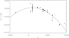 |
Fig. 1. O-C diagram with all the points collected from literature (see Table 7) and the resulting quadratic fit (continuous line). |
NSVS 10653195 eclipse times from the literature and from our IR photometry.
The new period change, obtained from the quadratic coefficient, is dP/dt = −(2.23 ± 0.24)×10−7 d yr−1, which is a typical value seen in other LMDEBs (see for example Lee et al. 2013). Since this is a well-detached binary system (see Sect. 4) this period change cannot be due to mass exchange between components.
NSVS 10653195 is composed of two active stars, and therefore a possible explanation for its period change could be angular momentum loss (AML) due to magnetic braking (Bradstreet & Guinan 1994). We computed the rate of period change produced by AML using Eq. (2) of Bradstreet & Guinan (1994) taking k2 = 0.1 and the results in Table 12. This resulted in (dP/dt)AML = −1.1 × 10⁻¹⁰ d yr−1, a value too low to account for the observed variation. Another possible explanation is the presence of a third body in the system in a long-period orbit. This would have to be a low-luminosity object, since no measurable third light is detected in this system (see Sect. 4.5). The third body scenario is also supported by the observation of regular period changes in other LMDEB attributed to substellar companions (Wolf et al. 2016). However, to confirm this possibility a periodic behavior in the O-C diagram is required, and this is not seen in this eclipsing binary.
4.4. Rotation and synchronicity parameter
We assumed that the two components of this system are tidally synchronized (Hut 1981). This is a reasonable assumption, as the synchronicity process is usually faster than the circularization process for convective envelope stars, and the secondary eclipse timings for the system of NSVS 10653195 suggest that the orbit is already circularized. As a result, the synchronicity parameters for this system were set to F1 = F2 = 1. This assumption is verified in Sect. 5.
4.5. Third light
Given the discrepancy between the optical and spectroscopic effective temperatures and the reported detection of a period variation, we searched extensively for a third light in this system. The existence of a third light could bias the mean color of the binary system to lower temperatures and is correlated with the inclination, since the eclipse depths of a system with third light can be reproduced with a similar system model but at lower inclination. All our tests, fitting for different Teff in the components, were also repeated fitting for third light with the other parameters, always with negative results. We also fitted the VRCIC LCs from Zhang et al. (2014) with and without third light, but the solutions were in all cases compatible with no third light.
4.6. Radial-velocity fit
The RV observations were fitted using the rvfit code, which can simultaneously fit the seven parameters of a double-line spectroscopic binary using an adaptive simulated annealing algorithm (see Iglesias-Marzoa et al. 2015, for details). For the case of NSVS 10653195 we adopted a circular orbit model, given that the secondary eclipse lies on phase 0.5. Thus, we fixed the eccentricity to zero and the argument of the periastron, which is undefined for a circular orbit, to ω = 90° to match the times of the eclipses.
Given that the orbital period is known from photometry, we fitted the remaining three parameters (γ, K1, K2) to the observations. Once the solution was found, we computed robust uncertainties in these three parameters using a Markov chain Monte-Carlo (MCMC) procedure. The fitted RV orbital solution is shown in Fig. 2 and the obtained parameters and derived physical quantities in Table 8. The value obtained for the mass ratio q = M2/M1 shows that the secondary component, that is, the one eclipsed at the photometric secondary minimum, is slightly more massive than the primary, despite having less surface luminosity.
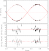 |
Fig. 2. Spectroscopic orbit (top panel) and residuals (bottom panel) resulting from the fit to the RVs observed by TRES. The eccentricity was fixed to zero according to a circular orbit. The resulting parameters are those of Table 8. The observations are plotted with their uncertainties, though in the top panel they have nearly the same size as the symbols. |
Radial-velocity fitting results.
The two deviating RV observations in the primary star RV curve near phase 0.36 caught our attention. We checked these spectra looking for abnormal features or for contamination from the Moon but nothing appeared to be out of the ordinary so we decided to keep them for the fit. The contamination from moonlight can bias the RVs because the extra lines from the reflected light from the Sun can be blended with the lines of the binary components to different degrees, thus distorting the line profiles and therefore affecting the determination of the centroids in the cross-correlation analysis. As a check, we repeated the fit without these two points and obtained values of γ = −16.52 ± 0.31 km s−1, K1 = 141.78 ± 0.49 km s−1, and K2 = 139.01 ± 0.49 km s−1, consistent within 1σ with the adopted solution. The resulting mass ratio from this solution is q = 1.0199 ± 0.0050, confirming that the secondary is more massive than the primary as before, and that the two points are not the cause of the q > 1 value.
Previous estimates of the q parameter reported in the literature give very different values, as they were done fitting only LCs. For detached eclipsing binaries the value of q is not constrained by the LCs, and it could happen that the value that numerically minimizes the merit function for the LCs does not correspond to the actual q value of the system. For example Zhang et al. (2015) did a search of the q value in the range 0.2−1.0, which resulted in q = 0.280 ± 0.004. The closest value of q found in the literature was obtained by Coughlin & Shaw (2007) who reported q = 0.91.
4.7. Light-curve fit
The VRIJK light curves described in Sects. 2.1 and 2.2 were fitted simultaneously using the 1.0 SVN version of PHysics Of Eclipsing BinariEs (PHOEBE, Prša & Zwitter 2005; Prša 2011). PHOEBE is a front-end of the well-known Wilson-Devinney code (WD, Wilson & Devinney 1971) which adds improvements to the treatment of multiwavelengh light curves. The WD employs a physical model of the gravitational distortions, radiative properties, and spot parameters of an eclipsing binary star. From preliminary fits we obtained fractional radii of r1 = r2 ≃ 0.22, and using q = 1.0170 from RV curves, we estimated the Roche lobe radii for each component as rL1 ≃ 0.35 and rL2 ≃ 0.36 using the Eggleton (1983) formula. These values are well above the relative radii r1 and r2 and therefore we selected a “detached eclipsing binary” model. To properly weight the fitting of each LC we measured the actual dispersion of each LC at quadratures (σV = 0.0047, σR = 0.0047, σI = 0.0058, σJ = 0.055, σK = 0.063) and weighted each LC with its σ value (curve-dependent weights). This gives more weight in the model fit to the more precise VRI LCs.
Given the large number of parameters, we fixed some of them using external data and constraints. The period and the epoch of the primary eclipse was fixed to the values of Eq. (2). The mass ratio q = M2/M1 and the system RV γ were fixed to those of the RV fit in Table 8. The eccentricity was fixed to e = 0.0 corresponding to a circular orbit. The synchronicity parameters for the two components were set to F1, 2 = 1.0 corresponding to tidally synchronized stars (Hut 1981).
The Teff1 was set to the adopted value of the mean temperature of the system as computed from the absolute photometry (4240 ± 100 K, see Table 6). The albedos were set to A1 = A2 = 0.5 following the prescription for stars with convective envelopes (Ruciński 1969). The gravity-brightening β1 and β2 exponents were both fixed to 0.32 as suggested by Lucy (1967). As a sanity check we computed the β values following the Claret (2000) study and obtained very similar values (β1 = 0.35 for Teff1 = 4240 K and β2 = 0.31 for Teff1 = 4120 K from preliminary fits).
We selected a square-root limb-darkening (LD) law since this is the one that better fits light curves at longer wavelengths and in the IR (Diaz-Cordoves & Gimenez 1992; van Hamme 1993). The LD coefficients were automatically computed after each iteration using the tables of van Hamme (1993). The third light was initially allowed to vary (l3 ≠ 0), but all our tests resulted in negative values or values compatible with no third light, and so in the final fits it was fixed to zero (see below). We also allowed for mutual heating effects between the components but they do not significantly affect the fit.
4.8. Spot modeling
The need to include spots in the LC model is evident in view of the modulation of the out-of-eclipse light curves. We made some preliminary tests placing spots in the two components at latitudes of ∼45°, given that there are hints that this is the range of latitudes most affected by spots in low-mass stars (Hatzes 1995; Granzer et al. 2000). The parameters of the spots, namely, latitude, longitude, radius, and temperature ratio (Tspot/Tsurf) were allowed to vary in order to fit the observed variations of the light curves. In these initial tests we tried several spot scenarios, including the use of bright spots (by forcing Tspot/Tsurf > 1) facing the observer at phase ∼0.2 to reproduce the hump observed at that phase. Finally, the best model was achieved with two dark spots (Tspot/Tsurf < 1) at convenient phases to mimic the effect of the a bright spot at the opposite side of the binary. With these two dark spots, the profile of the eclipses was much better reproduced, but small systematic residuals remained at phases surrounding the secondary eclipse, and so we placed another spot in the secondary star which fitted the residuals much better. Although PHOEBE can only fit two spots simultaneously, we managed to fit the three spots by fitting two of them at once and cycling between them until a satisfactory convergence was obtained. The model of NSVS 10653195 with spots in the two components is supported by the fact that the spectra show activity for the two components, since CaII H and K lines are clearly seen in emission in both stars. Visual inspection shows no difference in the height of the emission cores, which would suggest similar activity levels. We fitted other models with spots in only one component but they did not fit as well as the one with spots on the two stars.
4.9. Final solution
We fitted the PHOEBE model allowing to vary the following parameters: the phase shift Δϕ, the secondary effective temperature Teff2, the orbital inclination i, the two surface potentials Ω1, Ω2, the passband luminosities (HLA), and the spot parameters. The parameters obtained for the final solution are shown in Table 9. The uncertainties in this table are the formal ones from the PHOEBE fit, and they not include correlations among parameters or systematic effects. The formal uncertainty in Teff2 is about 4 K, but taking into account that the Teff1 uncertainty is ±100 K, we choose to add them in quadrature to take into account the dependence of the two values.
NSVS 10653195 parameters computed from the PHOEBE fit to the VRIJK differential light curves.
The rvol values are the volumetric radii from which the absolute radii can be computed. We note that the stars are only slightly distorted (rpoint/rpole ∼ 3.2% and 2.8% for the primary and the secondary, respectively) in spite of the proximity of the stars. The fitted light curves and their residuals are shown in Fig. 3.
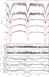 |
Fig. 3. Top panel: NSVS 10653195 light curves (points) and PHOEBE fitted model (red lines) with the parameters of Table 9. From top to bottom: K, J, I, R, and V differential light curves. K and J band TCS filters are displaced −0.7 and −0.1 magnitudes, respectively, for a better viewing. Lower panels: residuals of the fits in the same order as the light curves in the top panel. We note the different vertical scales of the panels. |
Figure 4 is a graphical representation of the spot configuration for four orbital phases of NSVS 10653195. It is possible that instead of extended spots (37, 21, and 29 degrees), each of them comprises a group of close smaller spots with higher Teff contrast with the surrounding photosphere, or even that they are spots with variable surface Teff distributions. However, with the present data, it is not possible to distinguish among these possibilities; this would require Doppler imaging observations (Strassmeier 2009) as was done before in the case of YY Gem (Hatzes 1995).
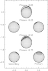 |
Fig. 4. Representation of the spot configuration of NSVS 10653195 in the (v, w) plane at four phases: from top to bottom, at the primary eclipse (phase 0.0), at the first quadrature (phase 0.25), at the secondary eclipse (phase 0.5), and at the second quadrature (phase 0.75). Both axes have units of relative radius and the images are displaced −0.60 from the previous one. The star in front is orbiting towards the right side and the primary star is the one with two spots. |
A drawback of the PHOEBE code, which comes from the WD code, is that it does not allow the radius ratio (r2/r1) to be fitted. In partially eclipsing systems with similar components, as is the case here, the radius ratio can often be poorly constrained and can be correlated with other parameters. An analysis of this behavior is described in Torres & Ribas (2002) for YY Gem. On the other hand, the sum of radii (r1 + r2) is well constrained by the duration of the eclipses, which can be measured with precision. Fitting separately for the individual radii (or the potentials) is not optimal. Since the radius ratio is always strongly correlated with the light ratio, it is often beneficial within MCMC to put a prior on the light ratio using the spectroscopic value, which indirectly constrains the radius ratio. However, this has to be done for the same mean wavelength of the spectra – in this case 5187 Å – and cannot be done in PHOEBE because the filter passbands do not match this wavelength.
Given that we assigned the mean effective temperature of the system to the primary star, the actual effective temperature of the primary must be hotter than the imposed value. To check whether or not the assumed Teff1 should be changed in a new analysis, we estimated the value of Teff1 using the PHOEBE results and the equations for the bolometric luminosity,  , and a similar equation for L2. The total bolometric luminosity of the system is
  , ST being the total surface of the two components, σ the Stefan-Boltzmann constant, and Teffm the mean effective temperature computed from the colors of the system. From these equations we can compute the mean Teffm as
![Mathematical equation: $$ \begin{aligned} T_{\rm eff m}=T_{\rm eff 1}\left[ \frac{1+L_2/L_1}{1+(L_2/L_1)(T_{\rm eff1}/T_{\rm eff2})^4} \right]^{1/4}\cdot \end{aligned} $$](/articles/aa/full_html/2019/07/aa35516-19/aa35516-19-eq16.gif) (4)
(4)
From the PHOEBE results in Table 9 we computed the radii R1 = 0.6907 ± 0.0038 R⊙, R2 = 0.6707 ± 0.0047 R⊙, and bolometric luminosities L1 = 0.139 ± 0.013 L⊙, L2 = 0.117 ± 0.012 L⊙. Using those values in Eq. (4) we obtained Teff1 = 4300 K for the primary component, which is within 1σ of the value in the previous fit, and we fitted again the LCs imposing this corrected Teff1.
The parameter values in Table 9 result in a distance to the system of d = 136.1 ± 6.9 pc, in very good agreement with the Gaia distance of 131.6 ± 0.8 pc (difference of 0.65σ). But from the parameters obtained from the new fit, fixing Teff1 = 4300 K, we estimated a distance d = 147.2 ± 6.8 pc, which is 2.3σ greater than the Gaia distance. In light of this result we prefer to maintain for the primary the initial Teff1 = 4240 ± 100 K. The difference in primary temperatures is well within the uncertainties in the mean photometric temperature. This check also discards the value of 4600 K suggested by the spectra of the system since the luminosity of a system with such Teff would put the binary much further away than is allowed by the constraint of the Gaia distance. All these tests were done fixing l3 = 0, and we repeated them by fitting for l3 with the other parameters. Again, this resulted in no detectable third light.
A second test was done fitting for the Teff of the two components exploiting the fact that the LCs span a wide range of wavelengths. The constraint on the individual temperatures are nevertheless too weak, and the fit resulted in two temperatures that are too low to account for the observed photometric colors. As before, this fit was also repeated fitting for a third light without positive results.
We checked the individual Teff of the two components using the relation among fundamental parameters of Mamajek (2015) and the calibration of Huang et al. (2015). We computed the absolute magnitudes for each component in several filters using the luminosity ratios for each passband in Table 9, the out-of-eclipse calibrated magnitudes of Table 5, the Gaia distance for the system, and the computed extinction for each passband. The resulting color indices are consequently corrected from extinction. The conversion from the Kron-Cousins to the Johnson photometric system for the optical bands was done using the relations given by Fernie (1983), while the conversion between the 2MASS system and the TCS system for the NIR bands was done using the transformation given by Ramírez & Meléndez (2005) for dwarfs. The results are given in Table 10 and show good agreement with the fitted effective temperatures for the two components.
Teff for the NSVS 10653195 system components computed using absolute magnitudes and color indices from the PHOEBE fitted model.
We also computed the individual Teff using the method of Ribas et al. (1998), adopting the V apparent magnitudes computed from the luminosity ratios (V1 = 13.461 ± 0.007, V2 = 13.749 ± 0.007), the Gaia parallax (π = 7.571 ± 0.042 mas), the interstellar extinction in the V band (AV = 0.063 ± 0.007), and the BC computed from Teff in Table 9 (BC1 = −0.83 ± 0.10, BC2 = −0.96 ± 0.12). They result in Teff1 = 4160 ± 100 K and Teff2 = 4070 ± 110 K, slightly lower but within 1σ agreement with the values and uncertainties from the fit.
The values of the uncertainties in the Table 9 are the formal ones of the PHOEBE fit. To compute robust estimations of the uncertainties for the fitted parameters we used a MCMC wrapper for PHOEBE (Prša, priv. comm.). We show the results of the computation at the bottom of Table 9. Figure 5 shows the parameter correlations from MCMC simulations and histograms of individual parameter marginalized distributions. The correlation between the two potentials Ω1 and Ω2 is clear and related to the problem with the determination of r2/r1 mentioned before.
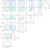 |
Fig. 5. Parameter correlations resulting from the MCMC fit and histograms of individual parameter distributions. The red vertical lines show the values adopted in this work from the maximum of the histograms. Dashed vertical lines indicate the 68.3% confidence intervals, which are the adopted uncertainties in the parameters. |
To ensure the robustness of the MCMC fitted light-curve model we ran Gelman-Rubin diagnostics (Gelman & Rubin 1992) on this group of parameters. In this test, a value near  indicates a robust solution of the MCMC. Table 11 shows the
  values for each fitted parameter.
Computed  values from the Gelman-Rubin test for the fitted parameters.
The most striking characteristic of this system is the inverted relation among the radii and the masses for the two components. Having very similar masses, the primary star is slightly less massive, but is larger and hotter. Based on the resulting spot configuration and on the similar intensity of emission of the CaII H and K lines, the two components display similar levels of activity, and so any radius inflation would be expected to be similar for the two stars. Also, radius inflation usually comes together with temperature suppression, meaning that if a star is inflated, it is also typically too cool. However, this is not seen in the results of the PHOEBE model for the primary. A primary larger than the secondary is seen in all our PHOEBE fits and in the MCMC simulation, and is also confirmed by the solutions of Coughlin & Shaw (2007), Wolf et al. (2010), and Zhang et al. (2014, 2015), the latter with independent data sets from ours. As a final test, we also independently fitted with PHOEBE the VRCIC light curves of Zhang et al. (2014) jointly with our RV results. For these light curves only a spot is needed over the primary to get a reasonable fit. The resulting model is again compatible with no third light, and it results in potentials Ω1 = 5.483 ± 0.014 and Ω2 = 5.716 ± 0.016 which translates again to r1 > r2.
5. The system of NSVS 10653195
5.1. Absolute parameters
The absolute parameters for the NSVS 10653195 system are shown in Table 12. They were computed from the results in Tables 8 and 9, adopting the Teff2, potentials Ω1 and Ω2, and orbital inclination with their uncertainties from the MCMC computation. The volumetric radii were computed solving Eqs. (1) and (2) of Wilson (1979). The adopted uncertainty in Teff2 was taken to be the combination of the MCMC uncertainties and the Teff1 uncertainty added in quadrature, the latter arising from the photometric colors and the empirical calibrations. For the solar values we used the recommended International Astronomical Union (IAU) values Teff⊙ = 5772 K, log g⊙ = 4.438, Mbol⊙ = 4.74 (IAU Inter-Division A-G Working Group on Nominal Units for Stellar & Planetary Astronomy 2015; Prša et al. 2016). The bolometric corrections (BC) were computed using the BC scale by Flower (1996) with the corrections given in Sect. 2 of Torres (2010).
Absolute dimensions and main physical parameters of the NSVS 10653195 system components.
Based on their effective temperatures, the two stars have spectral types K6V and K7V (Mamajek 2015). Given the uncertainties in the Teff we adopted uncertainties of ±1 for the spectral types. The masses both have relative uncertainties of σ(M)/M ≃ ±0.8%, while the radii have (+2.5%, −3.5%) for R1, and (+2.7%, −3.3%) for R2, which makes this system suitable for testing the stellar models. The departure of the two stars from a spherical model is very small with the two stars well inside their Roche lobes.
The physical parameters of this system suggest that the times for the tidal synchronization and orbital circularization to occur are very short (Hut 1981). Following Hilditch (2001), these times, in units of years, can be computed as
 (5)
(5)
 (6)
(6)
where q = M2/M1 is the mass ratio (from Table 8) and P is the orbital period in days. For NSVS 10653195 these times are tsync ≃ 103 yr and tcirc ≃ 4.5 × 10⁴ yr. These values are small compared to typical ages of low-mass stars, and justify our assumptions about the synchronicity parameters in Sect. 4.4.
5.2. Age, distance, and space velocities
Using the bolometric luminosities of the two components in Table 12, and bolometric corrections (BCV), we obtain a combined absolute V magnitude for the system of  . Using the visual apparent magnitude of the system (V = 12.843 ± 0.005, see Table 5) and the interstellar reddening in the V band, this results in a distance modulus of
  , which translates into a distance of
  pc. The computed distance to the system is in excellent agreement with the Gaia value (dGaia = 131.6 ± 0.8 pc) with the bulk of the uncertainty coming from the Teff and the bolometric corrections that arise from them.
We also computed the Galactic (U, V, W)5 space velocities applying the prescription of Johnson & Soderblom (1987), the systemic RV of the system (see Sect. 4.6), and the Gaia distance and proper motion measurements: μα = −37.938 ± 0.052 mas yr−1, μδ = −23.381 ± 0.051 mas yr−1. The resultant velocities are U = −10.07 ± 0.21 km s−1, V = −30.21 ± 0.18 km s−1, and W = −0.04 ± 0.22 km s−1, and a total space velocity of S = 31.84 ± 0.35 km s−1. These Galactic velocities indicate thin disk kinematics for NSVS 10653195, as the W velocity is nearly zero.
In an attempt to constrain the age of the system we checked a number of kinematic criteria with little success. This binary is outside the area defined by Eggen (1989) as belonging to the young Galactic disk, and the velocities lie just over the V boundary of the criteria of Leggett (1992) (−50 < U < 20, −30 < V < 0, −25 < W < 10, all in km s−1); also the binary is not within any known early-type or late-type population tracer (Skuljan et al. 1999), and cannot be related to any known moving group (Montes et al. 2001; Maldonado et al. 2010). Therefore, we cannot impose constraints on the age of the system based on kinematic criteria. In addition, the short period of this system cannot impose constraints based on the synchronization or the circularization times. At best, all we can say from this system, based on a solar or sub-solar metallicity and the typical age of K stars, is that the system would be a main sequence star with an undefined age of one or more gigayears.
At last, Fig. 6 shows a Mbol–log Teff diagram of the two components of this system with the Baraffe et al. (1998; hereafter BCAH98) isochrones overplotted. Since the metallicity of NSVS 10653195 is unknown we included isochrones for solar metallicity [M/H] = 0.0 dex represented as black lines, and for low metallicity with [M/H] = −0.5 dex, represented by red lines. Assuming solar metallicity, all that can we say from that figure is that this system is older than log (age(yr)) ∼ 8. Any age of log (age(yr)) ∼ 8 or older fits the two components equally well. In this scenario, NSVS 10653195 would be a main sequence system. If low metallicity is assumed, for example [M/H] = −0.5 dex, the age of the system could be fitted by a younger isochrone, with an age halfway log (age(yr)) = 7 − 8. Metallicities slightly over [M/H] = −0.5 could also fit an old system given the uncertainties in the position of the components in the Mbol–log Teff plane. Specific metallicity measurements for this system would help to resolve this ambiguity; though as mentioned before they would be difficult to measure because of their high rotation speeds.
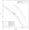 |
Fig. 6. Position in the Mbol–log Teff diagram of the NSVS 10653195 system components. BCAH98 isochrones are for [M/H] = 0.0 (black) and [M/H] = −0.5 (red) for log (age) = 6.0, 7.0, 8.0, 9.0 and 9.9. The ages of the components are compatible with log (age) = 8.0 and older or even with younger ages if the metallicity is lower than solar. |
5.3. Comparison with models
In Fig. 7 we plot the masses and radii for the NSVS 10653195 components and other benchmark LMDEBs collected from the literature. The individual components of benchmark LMDEBs are plotted as filled circles and the components of NSVS 10653195 are plotted as open diamonds. All of them are plotted with their uncertainties, but in many cases those are smaller than the plot symbols. It must be stressed that some of the systems taken from the literature quote only formal uncertainties and that actual error bars should be larger. The complete list of systems plotted can be found in Iglesias-Marzoa et al. (2017; see their Table 15) from which we selected those with relative uncertainties of less than 5% in mass and radius.
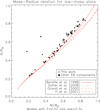 |
Fig. 7. Mass–radius relations of stars between 0.2 and 1.0 M⊙ predicted by four stellar models (see text). The filled circles represent well-known LMDEBs used as benchmarks for the models. The diamonds represent the location of NSVS 10653195 system components. The uncertainties in the parameters are represented by bars, though in many of the systems these are smaller than the symbols. Metallicity and age are set for reference of the whole set of stars and are not a fit to the NSVS 10653195 parameters. |
We also plotted four theoretical models which predict mass–radii relations for the stellar low-mass regime, namely the models of Baraffe et al. (1998), Dotter et al. (2008), Girardi et al. (2000), and Yi et al. (2001). The selected models have solar metallicity (Z = 0.02) and an age of 3 Gyr, and they must be taken only as reference and for comparison with the sample of objects. They are not fits to the components of NSVS 10653195. For the Baraffe et al. (1998) model we selected a mixing length parameter of α = l/Hp = 1.
The components of NSVS 10653195 follow the same trend seen in other LMDEBs in their range of masses, that is, the components are oversized with respect to the radius predicted by the models: the radius of the primary is about 15% larger than the model predicts, and the radius of the secondary is about 12% larger. Those differences are clearly larger than the computed radii uncertainties.
Figure 8 shows the mass–Teff relation for the same LMDEB systems plotted in Fig. 7 and for NSVS 10653195. In this case, the components of NSVS 10653195 are well represented by the stellar models; in particular, the Dartmouth model (Dotter et al. 2008) passes between the two components.
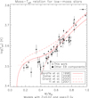 |
Fig. 8. Mass–log Teff relations for the same LMDEB systems as in Fig. 7. Metallicity and age are set for reference of the whole set of stars and are not a fit to the NSVS 10653195 parameters. |
6. Conclusions
We present a set of reliable physical parameters of the NSVS 10653195 system components based on optical and IR differential photometry and on spectroscopic RV observations. This LMDEB system is composed of two oversized main sequence K stars. The resulting physical parameters for the primary star are M1 = 0.6402 ± 0.0052 M⊙,  R⊙, and Teff1 = 4240 ± 100 K. For the secondary, the parameters are M2 = 0.6511 ± 0.0052 M⊙,
  R⊙, and
  K. The uncertainties in mass and radius were derived in a robust way using MCMC and are at the level of ∼0.8% for mass and ∼3% for radius, allowing for comparison with current models of low-mass stars. As seen for other LMDEBs, the components show inflated radii, and Teff depression is found at a similar level to that of other LMDEBs.
The orbit is circular with i = 86.22 ± 0.61 degrees and our derived distance is in excellent agreement with the value derived from Gaia parallax. This imposes a strict constraint on the luminosity of the system, and, as a result, on the effective temperature. We do not detect any hint of third light in our numerous tests on the LCs of this system. As a consequence, the period change reported by Zhang et al. (2015) is unlikely to be explained by the presence of a third main sequence body in the system, though a white dwarf or a substellar object is still possible. Both components show signs of activity in the form of spots and CaII H and K emission lines which complicates the analysis of the LCs. The age of the system cannot be established using isochrones or kinematical properties. Therefore, although unlikely given the typically old age of the stars in this mass range, a young system cannot be completely discarded.
We notice that the star labeled 1 in ELC is the one which is closest to the observer at primary (deepest) eclipse, usually at phase zero, and thus star 2 is eclipsed at that time. This labeling scheme is opposed to that used traditionally in light curves of eclipsing binaries, which we adopted. Thus, star 1 in ELC is the secondary component, labeled as 2 in this paper.
Positive values of U, V, and W indicate velocities toward the Galactic center, Galactic rotation, and north Galactic pole, respectively.
Acknowledgments
We thank the anonymous referee for their careful reading of the manuscript and helpful comments. This article is based on observations made with the Carlos Sánchez IR telescope (TCS) and the IAC80 optical telescope operated on the island of Tenerife by the Instituto de Astrofisica de Canarias in the Spanish Observatorio del Teide. Also is based on observations made with the Tillinghast Reflector Echelle Spectrograph (TRES) on the 1.5-meter Tillinghast telescope at the Smithsonian Astrophysical Observatory’s Fred L. Whipple Observatory. GT acknowledges partial support from the NSF through grant AST-1509375. RIM acknowledges support through the Programa de Acceso a Instalaciones Cientificas Singulares (E/309290). IRAF is distributed by the National Optical Astronomy Observatory, which is operated by the Association of Universities for Research in Astronomy (AURA) under a cooperative agreement with the National Science Foundation. This research has made use of the SIMBAD database, operated at CDS, Strasbourg, France, and of NASA’s Astrophysics Data System Bibliographic Services. Also, it used data products from the Two Micron All Sky Survey, which is a joint project of the University of Massachusetts and the Infrared Processing and Analysis Center, California Institute of Technology, and is funded by NASA and the National Science Foundation. We acknowledge the BRNO database for publishing their observations, and in particular to Katerina Honkova for her kind reply to our questions.
References
- Bahcall, J. N., & Soneira, R. M. 1980, ApJS, 44, 73 [NASA ADS] [CrossRef] [Google Scholar]
- Bailer-Jones, C. A. L., Rybizki, J., Fouesneau, M., Mantelet, G., & Andrae, R. 2018, AJ, 156, 58 [NASA ADS] [CrossRef] [Google Scholar]
- Bakos, G., Noyes, R. W., Kovács, G., et al. 2004, PASP, 116, 266 [NASA ADS] [CrossRef] [Google Scholar]
- Baraffe, I., Chabrier, G., Allard, F., & Hauschildt, P. H. 1998, A&A, 337, 403 [NASA ADS] [Google Scholar]
- Bilir, S., Ak, S., Karaali, S., et al. 2008, MNRAS, 384, 1178 [NASA ADS] [CrossRef] [Google Scholar]
- Borucki, W. J., Koch, D., Basri, G., et al. 2010, Science, 327, 977 [NASA ADS] [CrossRef] [PubMed] [Google Scholar]
- Bradstreet, D. H., & Guinan, E. F. 1994, in Interacting Binary Stars, ed. A. W. Shafter, ASP Conf. Ser., 56, 228 [NASA ADS] [Google Scholar]
- Buchhave, L. A., Bakos, G. Á., Hartman, J. D., et al. 2010, ApJ, 720, 1118 [NASA ADS] [CrossRef] [Google Scholar]
- Cabrera-Lavers, A., Garzón, F., Hammersley, P. L., Vicente, B., & González-Fernández, C. 2006, A&A, 453, 371 [NASA ADS] [CrossRef] [EDP Sciences] [Google Scholar]
- Casagrande, L., Ramírez, I., Meléndez, J., Bessell, M., & Asplund, M. 2010, A&A, 512, A54 [NASA ADS] [CrossRef] [EDP Sciences] [Google Scholar]
- Claret, A. 2000, A&A, 359, 289 [NASA ADS] [Google Scholar]
- Coughlin, J. L., & Shaw, J. S. 2007, J. Southeast. Assoc. Res. Astron., 1, 7 [Google Scholar]
- Coughlin, J. L., López-Morales, M., Harrison, T. E., Ule, N., & Hoffman, D. I. 2011, AJ, 141, 78 [NASA ADS] [CrossRef] [Google Scholar]
- Diaz-Cordoves, J., & Gimenez, A. 1992, A&A, 259, 227 [NASA ADS] [Google Scholar]
- Dotter, A., Chaboyer, B., Jevremović, D., et al. 2008, ApJS, 178, 89 [NASA ADS] [CrossRef] [Google Scholar]
- Drake, A. J., Djorgovski, S. G., Mahabal, A., et al. 2009, ApJ, 696, 870 [NASA ADS] [CrossRef] [MathSciNet] [Google Scholar]
- Eggen, O. J. 1989, PASP, 101, 366 [NASA ADS] [CrossRef] [Google Scholar]
- Eggleton, P. P. 1983, ApJ, 268, 368 [NASA ADS] [CrossRef] [Google Scholar]
- Fernie, J. D. 1983, PASP, 95, 782 [NASA ADS] [CrossRef] [Google Scholar]
- Flower, P. J. 1996, ApJ, 469, 355 [NASA ADS] [CrossRef] [Google Scholar]
- Fridlund, M., Baglin, A., Lochard, J., & Conroy, L. 2006, in The CoRoT Mission Pre-Launch Status – Stellar Seismology and Planet Finding, ESA SP, 1306 [Google Scholar]
- Fűrész, G. 2008, PhD Thesis, Univ. Szeged, Hungary [Google Scholar]
- Gelman, A., & Rubin, D. 1992, Stat. Sci., 7, 457 [Google Scholar]
- Girardi, L., Bressan, A., Bertelli, G., & Chiosi, C. 2000, A&AS, 141, 371 [NASA ADS] [CrossRef] [EDP Sciences] [Google Scholar]
- Glass, I. S. 1985, Ir. Astron. J., 17, 1 [NASA ADS] [Google Scholar]
- Granzer, T., Schüssler, M., Caligari, P., & Strassmeier, K. G. 2000, A&A, 355, 1087 [NASA ADS] [Google Scholar]
- Green, G. M., Schlafly, E. F., Finkbeiner, D., et al. 2018, MNRAS, 478, 651 [NASA ADS] [CrossRef] [Google Scholar]
- Hartman, J. D., Quinn, S. N., Bakos, G. Á., et al. 2018, AJ, 155, 114 [NASA ADS] [CrossRef] [Google Scholar]
- Hatzes, A. P. 1995, IAU Symp., 176, 90P [NASA ADS] [Google Scholar]
- Hilditch, R. W. 2001, An Introduction to Close Binary Stars, 1st edn. (New York: Cambridge University Press) [CrossRef] [Google Scholar]
- Honkova, K., Jurysek, J., Lehky, M., et al. 2015, Open Eur. J. Var. Stars, 168, 1 [NASA ADS] [Google Scholar]
- Huang, Y., Liu, X.-W., Yuan, H.-B., et al. 2015, MNRAS, 454, 2863 [NASA ADS] [CrossRef] [Google Scholar]
- Hut, P. 1981, A&A, 99, 126 [NASA ADS] [Google Scholar]
- IAU Inter-Division A-G Working Group on Nominal Units for Stellar & Planetary Astronomy 2015, Resolution B2 on Recommended Zero Points for the Absolute and Apparent Bolometric Magnitude Scales, Tech. Rep., IAU [Google Scholar]
- Iglesias-Marzoa, R., López-Morales, M., & Jesús Arévalo Morales, M. 2015, PASP, 127, 567 [NASA ADS] [CrossRef] [Google Scholar]
- Iglesias-Marzoa, R., López-Morales, M., Arévalo, M. J., Coughlin, J. L., & Lázaro, C. 2017, A&A, 600, A55 [NASA ADS] [CrossRef] [EDP Sciences] [Google Scholar]
- Irwin, J. M., Quinn, S. N., Berta, Z. K., et al. 2011, ApJ, 742, 123 [NASA ADS] [CrossRef] [Google Scholar]
- Johnson, H. L. 1966, ARA&A, 4, 193 [NASA ADS] [CrossRef] [Google Scholar]
- Johnson, D. R. H., & Soderblom, D. R. 1987, AJ, 93, 864 [NASA ADS] [CrossRef] [Google Scholar]
- Juryšek, J., Hoňková, K., Šmelcer, L., et al. 2017, Open Eur. J. Var. Stars, 179, 1 [NASA ADS] [Google Scholar]
- Kazarovets, E. V., Samus, N. N., & Durlevich, O. V. 1998, Inf. Bull. Var. Stars, 4655 [Google Scholar]
- Kochanek, C. S., Shappee, B. J., Stanek, K. Z., et al. 2017, PASP, 129, 104502 [NASA ADS] [CrossRef] [Google Scholar]
- Kwee, K. K., & van Woerden, H. 1956, Bull. Astron. Inst. Neth., 12, 327 [NASA ADS] [Google Scholar]
- Latham, D. W., Stefanik, R. P., Torres, G., et al. 2002, AJ, 124, 1144 [NASA ADS] [CrossRef] [Google Scholar]
- Law, N. M., Kulkarni, S. R., Dekany, R. G., et al. 2009, PASP, 121, 1395 [NASA ADS] [CrossRef] [Google Scholar]
- Lee, J. W., Youn, J.-H., Kim, S.-L., & Lee, C.-U. 2013, AJ, 145, 16 [NASA ADS] [CrossRef] [Google Scholar]
- Lee, C.-H., Koppenhoefer, J., Seitz, S., et al. 2014, ApJ, 797, 22 [NASA ADS] [CrossRef] [Google Scholar]
- Leggett, S. K. 1992, ApJS, 82, 351 [NASA ADS] [CrossRef] [Google Scholar]
- López-Morales, M. 2007, ApJ, 660, 732 [NASA ADS] [CrossRef] [Google Scholar]
- López-Morales, M., & Ribas, I. 2005, ApJ, 631, 1120 [NASA ADS] [CrossRef] [Google Scholar]
- Lucy, L. B. 1967, ZAp, 65, 89 [NASA ADS] [Google Scholar]
- Maldonado, J., Martínez-Arnáiz, R. M., Eiroa, C., Montes, D., & Montesinos, B. 2010, A&A, 521, A12 [NASA ADS] [CrossRef] [EDP Sciences] [Google Scholar]
- Mamajek, E. E. 2015, A Modern Mean Stellar Color and Effective Temperature Sequence for O9V–Y0V Dwarf Stars, http://www.pas.rochester.edu/emamajek/EEM_dwarf_UBVIJHK_colors_Teff.txt [Google Scholar]
- Mann, A. W., Brewer, J. M., Gaidos, E., Lépine, S., & Hilton, E. J. 2013, AJ, 145, 52 [NASA ADS] [CrossRef] [Google Scholar]
- Montes, D., López-Santiago, J., Gálvez, M. C., et al. 2001, MNRAS, 328, 45 [NASA ADS] [CrossRef] [MathSciNet] [Google Scholar]
- Morales, J. C., Gallardo, J., Ribas, I., et al. 2010, ApJ, 718, 502 [NASA ADS] [CrossRef] [Google Scholar]
- Nordström, B., Latham, D. W., Morse, J. A., et al. 1994, A&A, 287, 338 [NASA ADS] [Google Scholar]
- Orosz, J. A., & Hauschildt, P. H. 2000, A&A, 364, 265 [NASA ADS] [Google Scholar]
- Östensen, R. 2000, PhD Thesis, University of Trömso [Google Scholar]
- Östensen, R., & Solheim, J.-E. 2000, Balt. Astron., 9, 411 [NASA ADS] [Google Scholar]
- Pietrzyński, G., Graczyk, D., Gieren, W., et al. 2013, Nature, 495, 76 [NASA ADS] [CrossRef] [PubMed] [Google Scholar]
- Pojmanski, G. 1997, Acta Aston., 47, 467 [Google Scholar]
- Pojmanski, G. 1998, Acta Aston., 48, 35 [NASA ADS] [Google Scholar]
- Pollacco, D. L., Skillen, I., Collier Cameron, A., et al. 2006, PASP, 118, 1407 [NASA ADS] [CrossRef] [Google Scholar]
- Prša, A. 2011, PHOEBE Scientific Reference (Philadelphia: SIAM) [Google Scholar]
- Prša, A., & Zwitter, T. 2005, ApJ, 628, 426 [NASA ADS] [CrossRef] [Google Scholar]
- Prša, A., Harmanec, P., Torres, G., et al. 2016, AJ, 152, 41 [NASA ADS] [CrossRef] [Google Scholar]
- Ramírez, I., & Meléndez, J. 2005, ApJ, 626, 446 [NASA ADS] [CrossRef] [MathSciNet] [Google Scholar]
- Ribas, I., Gimenez, A., Torra, J., Jordi, C., & Oblak, E. 1998, A&A, 330, 600 [NASA ADS] [Google Scholar]
- Ribas, I., Jordi, C., Vilardell, F., et al. 2005, ApJ, 635, L37 [NASA ADS] [CrossRef] [Google Scholar]
- Ruciński, S. M. 1969, Acta Aston., 19, 245 [NASA ADS] [Google Scholar]
- Schlafly, E. F., & Finkbeiner, D. P. 2011, ApJ, 737, 103 [NASA ADS] [CrossRef] [Google Scholar]
- Schlegel, D. J., Finkbeiner, D. P., & Davis, M. 1998, ApJ, 500, 525 [NASA ADS] [CrossRef] [Google Scholar]
- Shaw, J. S., & López-Morales, M. 2007, in The Seventh Pacific Rim Conference on Stellar Astrophysics, eds. Y. W. Kang, H. W. Lee, K. C. Leung, & K. S. Cheng, ASP Conf. Ser., 362, 15 [NASA ADS] [Google Scholar]
- Skrutskie, M. F., Cutri, R. M., Stiening, R., et al. 2006, AJ, 131, 1163 [NASA ADS] [CrossRef] [Google Scholar]
- Skuljan, J., Hearnshaw, J. B., & Cottrell, P. L. 1999, MNRAS, 308, 731 [NASA ADS] [CrossRef] [Google Scholar]
- Šmelcer, L. 2019, BRNO Database, http://var2.astro.cz/EN/brno/index.php?lang=en [Google Scholar]
- Strassmeier, K. G. 2009, A&ARv, 17, 251 [NASA ADS] [CrossRef] [Google Scholar]
- Torres, G. 2010, AJ, 140, 1158 [NASA ADS] [CrossRef] [Google Scholar]
- Torres, G., & Ribas, I. 2002, ApJ, 567, 1140 [NASA ADS] [CrossRef] [Google Scholar]
- Torres, G., Neuhäuser, R., & Guenther, E. W. 2002, AJ, 123, 1701 [NASA ADS] [CrossRef] [Google Scholar]
- Torres, G., Andersen, J., & Giménez, A. 2010, A&ARv, 18, 67 [Google Scholar]
- van Hamme, W. 1993, AJ, 106, 2096 [NASA ADS] [CrossRef] [Google Scholar]
- Wilson, R. E. 1979, ApJ, 234, 1054 [NASA ADS] [CrossRef] [Google Scholar]
- Wilson, R. E., & Devinney, E. J. 1971, ApJ, 166, 605 [NASA ADS] [CrossRef] [Google Scholar]
- Wolf, M., Zejda, M., Mikulásek, J., et al. 2010, in Binaries – Key to Comprehension of the Universe, eds. A. Prša, & M. Zejda, ASP Conf. Ser., 435, 441 [NASA ADS] [Google Scholar]
- Wolf, M., Zasche, P., Kučáková, H., et al. 2016, A&A, 587, A82 [NASA ADS] [CrossRef] [EDP Sciences] [Google Scholar]
- Woźniak, P. R., Vestrand, W. T., Akerlof, C. W., et al. 2004, AJ, 127, 2436 [NASA ADS] [CrossRef] [Google Scholar]
- Yi, S., Demarque, P., Kim, Y.-C., et al. 2001, ApJS, 136, 417 [NASA ADS] [CrossRef] [Google Scholar]
- Zhang, L.-Y., Pi, Q.-F., & Yang, Y.-G. 2014, MNRAS, 442, 2620 [NASA ADS] [CrossRef] [Google Scholar]
- Zhang, B., Qian, S.-B., Liao, W.-P., et al. 2015, New A, 41, 37 [NASA ADS] [CrossRef] [Google Scholar]
- Zucker, S., & Mazeh, T. 1994, ApJ, 420, 806 [NASA ADS] [CrossRef] [EDP Sciences] [MathSciNet] [Google Scholar]
All Tables
Calibrated observed magnitudes and color indices for NSVS 10653195 obtained from our absolute photometry measurements.
Mean effective temperature estimations resulting from our BVRCIC photometry, and 2MASS photometry for NSVS 10653195.
NSVS 10653195 parameters computed from the PHOEBE fit to the VRIJK differential light curves.
Teff for the NSVS 10653195 system components computed using absolute magnitudes and color indices from the PHOEBE fitted model.
Absolute dimensions and main physical parameters of the NSVS 10653195 system components.
All Figures
|
Fig. 1. O-C diagram with all the points collected from literature (see Table 7) and the resulting quadratic fit (continuous line). |
| In the text | |
|
Fig. 2. Spectroscopic orbit (top panel) and residuals (bottom panel) resulting from the fit to the RVs observed by TRES. The eccentricity was fixed to zero according to a circular orbit. The resulting parameters are those of Table 8. The observations are plotted with their uncertainties, though in the top panel they have nearly the same size as the symbols. |
| In the text | |
|
Fig. 3. Top panel: NSVS 10653195 light curves (points) and PHOEBE fitted model (red lines) with the parameters of Table 9. From top to bottom: K, J, I, R, and V differential light curves. K and J band TCS filters are displaced −0.7 and −0.1 magnitudes, respectively, for a better viewing. Lower panels: residuals of the fits in the same order as the light curves in the top panel. We note the different vertical scales of the panels. |
| In the text | |
|
Fig. 4. Representation of the spot configuration of NSVS 10653195 in the (v, w) plane at four phases: from top to bottom, at the primary eclipse (phase 0.0), at the first quadrature (phase 0.25), at the secondary eclipse (phase 0.5), and at the second quadrature (phase 0.75). Both axes have units of relative radius and the images are displaced −0.60 from the previous one. The star in front is orbiting towards the right side and the primary star is the one with two spots. |
| In the text | |
|
Fig. 5. Parameter correlations resulting from the MCMC fit and histograms of individual parameter distributions. The red vertical lines show the values adopted in this work from the maximum of the histograms. Dashed vertical lines indicate the 68.3% confidence intervals, which are the adopted uncertainties in the parameters. |
| In the text | |
|
Fig. 6. Position in the Mbol–log Teff diagram of the NSVS 10653195 system components. BCAH98 isochrones are for [M/H] = 0.0 (black) and [M/H] = −0.5 (red) for log (age) = 6.0, 7.0, 8.0, 9.0 and 9.9. The ages of the components are compatible with log (age) = 8.0 and older or even with younger ages if the metallicity is lower than solar. |
| In the text | |
|
Fig. 7. Mass–radius relations of stars between 0.2 and 1.0 M⊙ predicted by four stellar models (see text). The filled circles represent well-known LMDEBs used as benchmarks for the models. The diamonds represent the location of NSVS 10653195 system components. The uncertainties in the parameters are represented by bars, though in many of the systems these are smaller than the symbols. Metallicity and age are set for reference of the whole set of stars and are not a fit to the NSVS 10653195 parameters. |
| In the text | |
|
Fig. 8. Mass–log Teff relations for the same LMDEB systems as in Fig. 7. Metallicity and age are set for reference of the whole set of stars and are not a fit to the NSVS 10653195 parameters. |
| In the text | |
Current usage metrics show cumulative count of Article Views (full-text article views including HTML views, PDF and ePub downloads, according to the available data) and Abstracts Views on Vision4Press platform.
Data correspond to usage on the plateform after 2015. The current usage metrics is available 48-96 hours after online publication and is updated daily on week days.
Initial download of the metrics may take a while.