| Issue |
A&A
Volume 627, July 2019
|
|
|---|---|---|
| Article Number | A91 | |
| Number of page(s) | 15 | |
| Section | Planets and planetary systems | |
| DOI | https://doi.org/10.1051/0004-6361/201935503 | |
| Published online | 04 July 2019 | |
Circumbinary discs with radiative cooling and embedded planets
Institut für Astronomie und Astrophysik, Universität Tübingen, Auf der Morgenstelle 10, 72076 Tübingen, Germany
e-mail: This email address is being protected from spambots. You need JavaScript enabled to view it.
Received:
20
March
2019
Accepted:
21
May
2019
Abstract
Context. As of today, ten circumbinary planets orbiting solar type main sequence stars have been discovered. Nearly all orbit around the central binary very closely to the region of instability where it is difficult to form them in situ. Hence, it is assumed that they formed further out and then migrated to their observed position, which is determined by binary, disc and planet properties.
Aims. We extend previous studies to a more realistic thermal disc structure and determine what parameter influence the final parking location of a planet around a binary star.
Methods. We performed two-dimensional numerical simulations of viscous accretion discs around a central binary. These simulations include viscous heating and radiative cooling from the disc surfaces. We vary the binary eccentricity as well as disc viscosity and mass.
Results. Concerning the disc evolution, we find that it can take well over 100 000 binary orbits until an equilibrium state is reached. As seen previously, we find that the central cavity opened by the binary becomes eccentric and precesses slowly in a prograde sense. Embedded planets migrate to the inner edge of the disc. In cases of lower disc viscosity they migrate further in maintaining a circular orbit, while for high viscosity they are parked further out on an eccentric orbit.
Conclusions. Discs around binary stars are eccentric, and precess very slowly around the binary. The final location of an embedded planet is linked to its ability to open a gap in the disc. Gap-opening planets separate inner from outer disc, preventing eccentricity excitation in the latter and making it more circular. This allows embedded planets to migrate closer to the binary, in agreement with the observations. The necessary conditions for gap opening and the final planet position depend on the planet mass and disc viscosity.
Key words: hydrodynamics / methods: numerical / binaries: general / accretion, accretion disks / protoplanetary disks
© ESO 2019
1 Introduction
Circumbinary discs are accretions discs that surround two central objects, such as a system of binary black holes or binary stars. In this study, we have dealt with protostellar discs that orbit around a binary system consisting of two protostars. We are interested in the dynamical evolution of such circumbinary discs and in addition we have studied the evolution of planets in these discs.
Approximately ten planets orbiting main sequence stellar binaries in a Tatooine-like manner have been discovered to date, all of them by the Kepler space telescope. The systems show planetary transits for both stars, hence are all very flat, an overview of their orbital parameter is given in Hamers et al. (2018) and references therein. This suggests a coplanar configuration of binary orbit and protostellar disc during the formation phase of the planetary systems. As a consequence, and to simplify the simulations, two-dimensional hydrodynamical studies of infinitesimally thin discs around binary stars are a good approximation. In this spirit, several simulations of circumbinary discs with and without embedded planets have been performed (Günther & Kley 2002; Pierens & Nelson 2007; MacFadyen & Milosavljević 2008), some with explicit reference to the observed Kepler systems (Pierens & Nelson 2013; Kley & Haghighipour 2014, 2015; Mutter et al. 2017a; Thun & Kley 2018).
Due to angular momentum transfer from the binary to the disc a central cavity develops where the density is strongly reduced. The size of this induced gap depends on disc parameters such as viscosity and pressure, and binary parameter such as orbital eccentricity and mass ratio (Artymowicz & Lubow 1994). Long-term high resolutions simulations have shown that the formed gaps around circumbinary stars feature a complicated dynamical evolution (Miranda et al. 2017; Thun et al. 2017; Thun & Kley 2018) with details depending on binary and disc parameter. In all cases the gap and the inner disc region turns eccentric and precesses slowly in a prograde manner around the binary star. Surprisingly, the highest gap eccentricity develops for circular binaries. Upon increasing the binary eccentricity, ebin, the gap first become more circular and then more eccentric again above a critical value of ebin ≈ 0.16 (Thun et al. 2017). Varying the binary mass ratio shows that for more-equal mass binaries the precession period increases for all binary eccentricities. Results of sequences of simulations for different binary parameter are shown in Thun & Kley (2018), where the overall variation of the gap orbital dynamics is compared to test particle trajectories around the binary.
Despite the formation of the gap the central binary can still accrete material from the disc that flows into the gap and is added onto central circumstellar discs. This mass flow within the cavity around the stars has been studied in a several simulations (Artymowicz & Lubow 1994; Günther & Kley 2002; Hanawa et al. 2010; de Val-Borro et al. 2011). The gas dynamics near the central objects is relevant in another example of circumbinary discs that refers to a central binary black hole system which is orbited by a disc, for example after a merger process of two galaxies in the early Universe. Of particular interest in this case is the evolution of the orbital elements of the binary as it accretes mass and angular momentum from the disc and exchanges angular momentum with the disc via gravitational torques. While earlier studies find a decrease of the orbit of the binary due to the angular momentum loss to the disc (Cuadra et al. 2009), recent work suggests that an expansion of the binary orbit due to mass and accompanying angular momentum accretion is also possible (Miranda et al. 2017; Muñoz et al. 2019). As we are interested here in the overall long-term evolution and structure of the disc we do not study the central region in this work and leave this interesting topic to future investigations.
The detected circumbinary planets all orbit the binary star close to the dynamical instability limit (Quarles et al. 2018). The strong dynamical action of the binary makes an in situ formation at this close vicinity very difficult and it is typically assumed that the planets formed further out in the disc and then migrated to their present location. Indeed, simulations of embedded planets show that they migrate inwards due to the planet disc interaction and then are “parked” at the inner disc edge, which is the outer rim of the gap (Pierens & Nelson 2007, 2008, 2013; Kley & Haghighipour 2014). Its final location is determined by the size andstructure of the central cavity region which depends, as mentioned above, on binary as well as disc parameter.
Most of the studies on circumbinary disc dynamics work with a simplified thermodynamical model using a locally isothermal disc structure where the temperature (or sound speed) in the disc is a given function of radius. As the few exceptions (Günther & Kley 2002; Kley & Haghighipour 2014) suffer from low numerical resolution or too short a time span, we have performed here a detailed study of the disc structure including viscous heating and radiative cooling from the disc surfaces. Starting from two baseline models using Kepler-16 and Kepler-38 parameter we varied binary eccentricity as well as disc mass and viscosity, and computed the disc evolution until an equilibrium state is reached. Finally, we embedded planets into the discand follow their evolution. We show that the final position of the planet is determined by its ability to open its own gap in the disc.
The paper is organised as follows: in Sect. 2 we describe the assumptions of our physical and numerical model. This is followed in Sect. 3 by a description of the structure of radiative circumbinary discs, for various binary eccentricities and different values for the disc viscosity. The evolution of an embedded planet in a radiative disc using Kepler-38 parameter is presented in Sect. 4. Our results are finally discussed in Sect. 5 and summarised in Sect. 6.
2 Model setup
We extended our previous locally isothermal circumbinary disc models (Thun et al. 2017; Thun & Kley 2018) to a more realistic equation of state, studied the impact on the disc structure and dynamics, and followed the orbital evolution of an embedded planet. We performed two-dimensional (2D) hydrodynamical, viscous simulations including an energy equation. To account for energy losses and prevent the disc from overheating by viscous dissipation we consider also radiative cooling from the disc surfaces. We studied the evolution of two sample systems: Kepler-16 and Kepler-38. The parameters of these two systems are summarised in Table 1.
2.1 Physical model
To model the circumbinary discs we used cylindrical coordinates (R, φ, z) centred on the centre of mass (COM) of the binary with the disc lying in the z = 0-plane. The observed Kepler systems with a circumbinary planet are nearly coplanar which justifies to work in 2D. We therefore assumed that the vertical extent of the disc, H, is small compared to the radial extension, and use the vertically averaged hydrodynamical equations, see Fig. 1. To be concise, we briefly quote only the main equations solved, and will refer to our previous studies for further detail.
The continuity equation is given by
 (1)
(1)
with the surface density  (see Fig. 1) and the 2D velocity
  . The vertically averaged equation of momentum conservation is given by
 (2)
(2)
with the vertically integrated pressure,  , and viscous stress tensor Π. The individual components in cylindrical coordinates are given in Kley (1999) or Masset (2002), where we have used here a vanishing bulk viscosity. To model the turbulent shear viscosity in the disc we used the standard α-disc model by Shakura & Sunyaev (1973). In this approximation, the kinematic viscosity coefficient can be written for thin discs as
 (3)
(3)
with a parameter α < 1, the adiabatic sound speed of the gas cs, and the vertical pressure scale height (disc half thickness) H.
The gravitational acceleration, g, acting on each cell due to the binary and the planet is given in detail described in Thun & Kley (2018) and we do not go into details here. It is given by the sum of the gravitational forces of the two binary stars, a possible planet and takes into account a possible acceleration of the COM of the binary. The gravitational acceleration contains a smoothing length ϵH to avoid singularities and to account for the correct treatment of the three-dimensional gravity in our 2D setup (Müller et al. 2012). In all simulations we use ϵ = 0.6 (Masset 2002) and evaluate the pressure scale height, H, at the location of the cell. Assuming a vertical hydrostatic equilibrium and an isothermal disc in the z-direction the disc height is given by
![Mathematical equation: \begin{equation*}H = \sqrt{\frac{P}{\Sigma}} \, \left[\sum_{\ell} \frac{G M_{\ell}}{\left| \bm{\mathrm{R}} - \bm{\mathrm{R}}_{\ell} \right|^3} \right]^{-1/2}, \end{equation*}](/articles/aa/full_html/2019/07/aa35503-19/aa35503-19-eq7.png) (4)
(4)
where R denotes the position of the grid cell and Rℓ the position of a star or planet. The summation in Eq. (4) runs over all gravitating objects (stars and planets). In the approximation Rℓ → 0, for large distances from the binary, this simplifies to
 (5)
(5)
where the mass of the binary is Mbin = MA + MB. We carried out test simulations to compare the sophisticated disc height (4) to the simple disc height (5), and did not find any significant differences. Therefore, in all our simulations we have used Eq. (5) to calculate the height of the disc.
The vertically averaged equation of energy conservation reads
![Mathematical equation: \begin{equation*}\frac{\partial}{\partial {t}}\left(\Sigma e\right) + {\bm{{\nabla}}} \cdot \left[\left(\Sigma e + P - \bm{{\Pi}} \right) \bm{\mathrm{u}} \right] = \left(\Sigma \bm{\mathrm{u}} \right) \cdot \bm{\mathrm{g}} - Q_-. \end{equation*}](/articles/aa/full_html/2019/07/aa35503-19/aa35503-19-eq9.png) (6)
(6)
The total specific energy e is related to the pressure by
 (7)
(7)
with the adiabatic index γ. In all our simulations we use a value of γ = 1.4. The pressure is related to the midplane temperature T of the disc
 (8)
(8)
with the Boltzmann constant kB, the mass of the hydrogen atom mH and the mean molecular mass of the gas μ (we use μ = 2.35). The adiabatic sound speed of the gas is then given by
 (9)
(9)
To model the cooling term Q− we followed D’Angelo et al. (2003) and Müller & Kley (2012) and only considered the cooling effect of radiation in the vertical direction and neglect radiation transport in the disc midplane. This is a good assumption if the vertical extent of the disc is small compared tothe discs’ radial extent. The cooling term models the energy loss by radiation from the upper and lower disc surface and can be written as
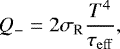 (10)
(10)
with the Stefan-Boltzmann constant σR. Since radiation can escape on both sides of the disc the factor of two in Eq. (10) is necessary. To calculate the effective optical depth τeff we followed an approach by Hubeny (1990) as given in Müller & Kley (2012).
 (11)
(11)
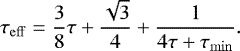
For the mean optical depth we used the following approximation
 (12)
(12)
where ϱ0 denotes the midplane gas density and  is a constant to account for the drop of opacity with vertical height in our two dimensional simulations (Müller & Kley 2012). To calculate the Rosseland mean opacity κ we assumed a power-law dependence on temperature and density (Lin & Papaloizou 1985)
 (13)
(13)
where ϱ0 and T refer to the midplane gas density and temperature. The values of κ0, a, and b for different opacity regimes can be found in a table given in Müller & Kley (2012). Figure 2 shows the opacity variation with temperature for three different densities. To calculate the opacity we used a function that smoothly transitions from one regime to another. We applied a minimum optical depth of τmin = 0.1 to account for the very optically thin regions of the disc.
In our simulations we have not considered the self-gravity of the disc as we are primarily interested in the end phase of the planet migration process when the disc mass is already reduced. For simulations of discs with self-gravity and embedded planets, see Mutter et al. (2017b,a). We also have not considered stellar irradiation, which we discuss in Sect. 5.3.
Orbital parameter of the stellar binaries in the Kepler-16 and Kepler-38 systems.
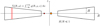 |
Fig. 1 Sketch of our disc model with the averaging process indicated for the three-dimensional density ϱ. The orange circle marks the primary and the red circle the secondary star for the Kepler-38 system, where the sizes are proportionalto the stellar masses. The origin of the coordinate system lies at the barycentre of the binary. |
 |
Fig. 2 Variation of the Rosseland mean opacity with temperature for three different densities ϱ. |
2.2 Initial conditions
For the initial disc parameters we followed Thun & Kley (2018) and use an initial surface density profile given by
 (14)
(14)
The function fgap models the expected cavity created by the binary (Artymowicz & Lubow 1994; Günther & Kley 2002)
![Mathematical equation: \begin{equation*} f_{\mathrm{gap}} = \left[1+\exp{\left(-\frac{R-R_{\mathrm{gap}}} {\Delta R}\right)} \right]^{-1} , \end{equation*}](/articles/aa/full_html/2019/07/aa35503-19/aa35503-19-eq19.png) (15)
(15)
with Rgap = 2.5 abin and ΔR = 0.1 Rgap. The reference density Σref is calculated according to the disc mass Mdisc inside the computational domain, and typically we have used a total initial disc mass of 0.01Mbin (for details see Thun & Kley 2018, Sect. 2.2). For the pressure profile we assumed a disc with an initial constant aspect ratio h(t = 0) = H ∕ R = 0.05 and calculate the initial pressure from Eq. (5)
 (16)
(16)
The initial radial velocity is set to zero uR(t = 0) = 0 and the initial azimuthal velocity is set to the local Keplerian velocity with respect to the COM of the binary  .
.
2.3 Numerical considerations
All simulations were performed by a modified version of PLUTO 4.2 (Mignone et al. 2007) which runs on graphical processor units (GPUs) and has in addition a N-body module to simulate the motion of planets in binary stars. Details can be found in Thun & Kley (2018) The new implementation of the cooling terms into the code is described in Appendix A. An overview of the numerical options for the hydrodynamical solver used here is given in Thun et al. (2017, Sect. 3.1). The numerical setup is identical to the setup described in Thun & Kley (2018, Sect. 2.3). We used a logarithmically expanding grid in the radial direction from Rmin = 1 abin to Rmax = 40 abin and a uniform grid from 0 to 2π in the azimuthal direction. In all our simulations this domain is covered by a grid with fixed resolution of Nr × Nφ = 684 × 584 cells. At Rmin a zero-gradient boundary condition (∂ ∕ ∂R = 0) is used for surface density, radial velocity, angular velocity Ωφ = uφ ∕ R, and pressure. Additionally, no inflow into the computational domain is allowed at Rmin. At Rmax we set the azimuthal velocity to the Keplerian velocity. For surface density and radial velocity we used a wave damping boundary condition, where uR is damped towards zero and Σ to the initial value (de Val-Borro et al. 2006; Thun & Kley 2018). For the pressure, again we used a zero-gradient boundary condition. In the azimuthal direction we use periodic boundary conditions. For stability reasons we used a global density floor of
 (17)
(17)
for a discussion of this value see Thun & Kley (2018). To enhance numerical stability we also use a temperature floor of Tfloor = 3 K and a temperature ceiling of Tceiling = 3000 K. The lower value prevents material from too low temperatures while the upper ceiling is relevant in the initial phase of the simulations in order to prevent too large temperatures in the inner gap region.
3 Disc structure
In this section we focus on the disc structure created by the gravitational interaction between the binary and the disc. We are interested in the size and eccentricity as well as the precession period of the gap as a function of binary eccentricity and physical disc properties. First, we describe a sequence of models for a fixed binary mass ratio qbin = 0.29 as in the Kepler-16 system, and vary the binary eccentricity ebin. As the thermodynamics of the disc are determined by the disc mass and viscosity we subsequently present models that use the fixed binary parameter of Kepler-38 for different Mdisc and viscosity α. The orbital parameter of Kepler-16 & 38 are listed in Table 1.
 |
Fig. 3 Time evolution of the disc eccentricity and mass for fixed qbin = 0.29 (as in Kepler-16) and various binary eccentricities over time. Top panel: disc eccentricity. Bottom panel: total mass in the disc in units of the central binary mass. |
3.1 Models for different binary eccentricity
For the model sequence presented in this section we use a fixed disc viscosity α = 0.001 and an initial disc mass of 0.01 Mbin. The total mass and mass ratio of the binary are those of the Kepler-16 system as quoted in Table 1. We ran a sequence of models for various binary eccentricities running from ebin = 0 to ebin = 0.28.
In Fig. 3 we display the evolution of the disc mass and eccentricity for various ebin over time. The top panel shows the disc eccentricity, where an averaging has been performed over the inner disc area out to a radius of R = 8.0 abin (Thun et al. 2017). The bottom panel shows the time evolution of the total disc mass in units of the central binary mass. The very long time needed until the disc reaches a quasi-equilibrium state is clearly noticable. However, this timescale depends on the binary eccentricity. For ebin larger than about 0.16 the discs settle in less than 100 000 Tbin while for lower ebin the equilibration time well exceeds 150 000 Tbin.
The discs around more circular binary stars with ebin < 0.1 show a larger disc eccentricity, edisc. The minimum of edisc is reached around ebin = 0.16 with a small increase for larger ebin. The mass loss from the disc through the inner boundary is moderate overall, during the 200 000 Tbin the total mass loss is at most 15%. In the very early phase, the mass loss is larger for the more eccentric binaries because the secondary periodically approaches the inner edge of the disc “pulling out” some material from it. Upon the strong increase of the disc eccentricity, particularly for the ebin = 0 model, the mass loss increases suddenly. In the long run all the models settle to a stationary state, as the density at the outer radius of the disc is held fixed at its initial value. During this adjustment phase the disc mass can also increase as the fixed density at Rmax serves as a mass reservoir for the inner disc.
In Fig. 4 we display the evolution of the gap geometry for the same models over time. The properties of the gap are here obtained by fitting an ellipse to the inner gap edge, where the density has reached about half of the maximum density near the inner rim of the disc. The exact procedure is described in Thun et al. (2017), and examples of such fitted ellipses are shown in Fig. 10 below. The time evolution of the obtained semi-major axis, eccentricity, and precession period of the ellipses are shown in Fig. 4. The horizontal lines in the figure and the labels indicate the values measured in the final phase of the simulations. The long process of finding the equilibrium is seen clearly in the lower two panels. In all models the gap size and eccentricity increase initially very strongly, reach their maxima between 20 000 and about 60 000 Tbin, and then settle slowlytowards equilibrium. The final gap eccentricities (bottom panel) are largest for the circular binary, reach the minimum at ebin = 0.16 and then increase again. The variation of the gap semi-major axis (middle panel) follows the same trend: the largest gap sizes are seen for low ebin and the smallest for ebin = 0.16. As seen from the top panel in the figure, the precession rate of the ellipse becomes very long for the discs with large gaps, and reach over 10 000 Tbin for the smaller ebin cases. Eventually, the precession period settles to values between about 2300 and 4770 Tbin for all models. This disc evolution is different to that of the locally isothermal discs presented in Thun & Kley (2018). In that study we did not observe the initial strong increase in the hole size and eccentricity. We comment on this difference in Sect. 5.2.
The time evolution for the disc eccentricity in Figs. 3 and 4 displays oscillatory behaviour for edisc or egap, respectively. The oscillations are a secular effect, they have been seen already in Thun et al. (2017) and discussed in Miranda et al. (2017). The oscillation period is identical to the precession period of the disc, that is, the time for one 360° turn of the eccentric disc. Similar to single test particle orbits, the period of the oscillations becomes longer for larger cavity sizes (corresponding to larger distances of the particle) and shorter for smaller cavities (Thun et al. 2017). This explains why the oscillations are wider in the early phase with the extended gap size, and are narrower in the relaxed equilibrium state.
The azimuthally averaged radial profile of various disc quantities are shown in Fig. 5 for the Kepler-16 case with ebin = 0.16 at five evolutionary times. The initial model is shown as a reference. The next two models at 10 000 and 60 000 Tbin demonstrate the early adjustment phase, and the two final models at 120 000 and 180 000 Tbin that the disc has indeed reached its equilibrium state. While initially the disc experiences a phase with a large eccentric gap, in the final state, the surface density is identical to the initial state beyond about 7abin. The disc’s averaged inner edge (about half value of Σpeak) always lies around 4 abin. Overall, the radiative disc is cooler than the initial setup with a reduced thickness. In the disc’s inner regions inside of about 15 abin the thickness is about H ∕ R = 0.04 while in the outer regions the thickness reduces to H ∕ R = 0.02. Within the gap the minimum thickness is, again about H ∕ R = 0.01−0.02. In the very inner parts of the disc near the inner boundary where the density is very close to the density floor, the temperature increases strongly, but still remains below the initial value corresponding to H ∕ R = 0.05. This increase in temperature is a numerical artefact and is discussed in more detail in Appendix A. Due to the very small density and pressure this hot gas does not have any dynamical influence on its environment. In the equilibrium state the disc’s eccentricity (bottom panel) reaches about 0.3 at the inner disc edge (at 3 abin) and is nearly circular beyond 15 abin.
In Fig. 6 we display the azimuthally averaged radial disc profiles for different ebin after 180 000 binary orbits. At this time, all models have reached the final equilibrium configuration. As could be already inferred from the calculated gap semi-major axis, in the models with smaller ebin, the maximum of the surface density lies further out in the disc and the peak value is very small. The turning point model with the smallest inner hole, for ebin = 0.16, has the largest density spike which lies closest to the binary. Due to the higher density, the disc is optically thicker and the midplane temperature is higher for the models with larger ebin. The temperature maxima for all models lie within the range 4–7 abin, well inside of the peak density. For the models with the larger binary eccentricities, the temperature peak coincides with the maximum of viscous dissipation at around 4−5 abin, as indicatedin the bottom panel in Fig. 6. For the dissipation function we considered only the Rφ-component of the viscous stress tensor
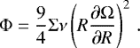 (18)
(18)
For the small binary eccentricities the temperature maximum is shifted to larger radii due to additional contributions by shock heating which is given by the term − P ∇⋅u. The disc eccentricity follows the same trend as the gap eccentricity. For smaller ebin the discs are more eccentric over a larger radial domain.
In Fig. 7 we display the gap precession period against gap size for models with identical qbin = 0.29 and varying ebin. The models for small ebin have large holes and long precession periods. Increasing ebin reduces the gap size and ellipticity and makes the disc precess faster. The turning point at which this trend reverses again, occurs at a critical value of ebin = 0.16. This value is identical to the critical point obtained for locally isothermal discs (with H ∕ R = 0.5) and with a viscosity of α = 0.01, as shown in the bifurcation diagram in Thun & Kley (2018). For this radiative disc, the upper and lower branches lie very close to each other. Scaling the precession period with the free particle orbits, as in Thun & Kley (2018), would separate the branches vertically.
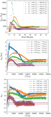 |
Fig. 4 Evolution of the gap properties for fixed qbin = 0.29 and various binary eccentricities. Top panel: precession period of the gap as a function of period number. Bottom two panels: semi-major axis and eccentricity of the gap. The horizontal lines and labels indicate the final values. |
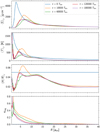 |
Fig. 5 Azimuthally averaged radial disc profiles for ebin = 0.16 at various evolutionary times. Displayed are the surface density, the midplane temperature, the disc thickness, and the disc eccentricity. |
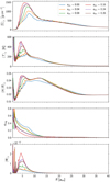 |
Fig. 6 Azimuthally averaged radial disc profiles in equilibrium for different ebin after 180 000 binary orbits. Displayed are the surface density, the midplane temperature, the disc thickness, the disc eccentricity, and in code units the dissipation function (18). |
3.2 Models for different disc masses and viscosities
For radiative models the disc evolution will be influenced by the total disc mass Mdisc and the viscosity α of the disc as these alter the disc temperature and hence change the dynamics. To estimate the impact that these parameters have on the disc structure we calculated models with different disc masses and viscosity. For the basic binary system we chose here Kepler-38, with the stellar masses and binary eccentricity given in Table 1.
To cover various disc physics, altogether we performed four simulations, with two different values for the viscosity, α =0.001 and 0.01, and two different initial disc masses, Mdisc = 0.01Mbin and 0.0057 Mbin. Figure 8 summarises the evolution of the dynamical gap properties in the four cases. As noted for the previous model sequence using Kepler-16 parameter, here all four simulations initially produce a large inner gap which becomes very eccentric with peak values reached after 40 000 to 60 000 binary orbits. After this, the inner gap shrinks and becomes more circular and settles to an equilibrium after about 100 000 Tbin. Discs with high viscosity (α = 0.01, blue and orange curves in Fig. 8) initially develop larger, and more eccentric gaps with precession periods above 15 000 Tbin. Reducing the viscosity by an order of magnitude (α = 0.001, red and green curves in Fig. 8) does not produce so large and eccentric gaps in the beginning. Both the gap size and eccentricity are near maximum approximately 30% smaller compared to the high viscosity case. The precession period of these low viscosity discs is still long and about 8000–10 000 binary orbits in the early phase. During the subsequent evolution all disc models settle to a dynamically similar final state after about 100 000 Tbin, with gap semi-major axes of agap = 4 abin and egap between 0.3 and 0.4, depending on α.
The evolution of the disc mass for the models is quoted in Fig. 9. The two models with the high viscosity, α =0.01, loose mass at a higher rate which is due to the higher viscosity and to the larger eccentricity of the disc which causes material to be lost through the inner boundary. After the quasi-equilibrium states have been reached, the mass loss from the disc into the inner hole becomes comparable for all cases. Compared to locally isothermal models with the same viscosity (as presented in Thun & Kley 2018) the radiative models tend to lose more mass. This could be due to the increased disc eccentricity in the radiative case. Highly eccentric orbits in the inner part of the disc come very close to the open inner boundary and gas on these orbits can easily flow through the open inner boundary. In contrast to the disc mass evolution presented in Fig. 3 where we see a slight mass increase in the end, we see here a continuous drop in disc mass. The overall evolution of the total disc mass in the domain is difficult to predict a priori. It depends on the initial mass in the disc which is not the same for the different cases. The models for Kepler-38 contain initially a higher disc mass (0.012 M⊙) compared to the Kepler-16 models (0.00089 M⊙) such that they lose more mass to reach equilibrium.
The two-dimensional density distribution of the central region at a time t = 88 000 is displayed in Fig. 10. For two models with the smaller viscosity (left panels) the surface density is lower than for theother two due to larger mass loss from the disc. The dashed white line corresponds to an elliptical fit to the approximate size and shape of the inner hole. The method of calculation of the approximate ellipse is described indetail in Thun et al. (2017). As mentioned above, all four models end in a dynamically comparable configuration.
The azimuthally averaged radial disc profiles are displayed in Fig. 11 after 120 000 binary orbits when all models have reached equilibrium. The two low viscosity models are shown in red and green, and the two high viscosity models in blue and orange. Due to the increased mass loss through the open inner boundary for high viscosity models the surface density (top panel) is reduced, while the lower α =0.001 models show a more pronounced density maximum. The second panel in Fig. 11 shows the midplane temperatureof the disc. The temperature peaks near the inner rim of the disc just inside of the density maximum due to viscous dissipation. As shown in the third panel of Fig. 11, the models with the higher initial disc mass show a final temperature above the starting configuration which corresponds to H ∕ R = 0.05, while the models with lower mass lie below it. Where the density rapidly drops inside the gap, the cooling is very effective, leading to very low temperatures. This behaviour is in agreement with Kley & Haghighipour (2014). In the very inner regions, close to Rmin we see again a strong increase in temperature which is due to numerically inaccurate cooling (see Appendix A, where we describe a possible solution). This feature has no dynamical impact due to the very low densities. In the outer part of the disc the behaviour of the temperature depends on the viscosity. For discs with high viscosity the viscous heating is more effective than the cooling and the temperature is slightly increased above the low viscosity models. We discuss the issue of irradiation (black dotted line in the second panel) in Sect. 5.3.
We notethe larger disc eccentricity of the model with high viscosity and disc mass, in particular in the outer regions of the disc. We do not have a full explanation for this behaviour but we believe that it is related to the different history of the model. Due to the larger disc mass, the temperature is higher than for the model with the same viscosity and lower mass (in orange). This causes sound waves to propagate faster through the disc, increasing the interaction with the outer boundary at Rmax. In the corresponding temperatureand H∕R distributions there is indeed some variation seen near the outer boundary which supports this reasoning.
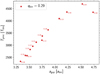 |
Fig. 7 Gap precession period against gap size in equilibrium after 180 000 binary orbits. All the models have the same qbin = 0.29 and differentebin as indicated by the labels. |
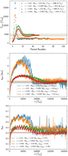 |
Fig. 8 Precession period, semi-major axis, and eccentricity of the disc gap vs. time, for discs with two different disc masses and viscosities. For the central binary we used the parameter of Kepler-38. The horizontal lines indicate time averages starting at 120 000 binary orbits, the time when all discs reached a quasi-steady state. |
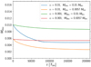 |
Fig. 9 Disc mass a function of time for models with different viscosity and disc mass. |
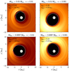 |
Fig. 10 Two-dimensional density distribution of the inner disc region at a time t = 88 000. The dashed white lines and labels correspond to the approximate sizes and shapes of the inner holes. The green arrow points towards the peri-centre of the binary and the orange arrow towards the pericentre of the inner gap. |
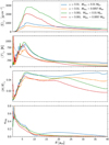 |
Fig. 11 Azimuthally averaged radial disc profiles for the different models of the Kepler-38 like system after 120 000 binary orbits. Displayed are the surface density, the midplane temperature, the disc thickness and the disc eccentricity. The black dotted line in the second panel represents the irradiation temperature of a sun-like star. |
Orbital parameter of the planet in the Kepler-38 system.
4 Planet evolution
In addition to studying the disc dynamics alone, we now add a planet to the last four simulations of the Kepler-38 system and follow its evolutionthrough the disc. The planet, with the observed mass of Kepler-38b (see Table 2), is embedded after 88 000 binary orbits into the system. At this time, the discs have approximately reached their equilibrium configurations, the corresponding 2D density distribution is shown in Fig. 10. To reduce the simulation time, the planet’s starting position lies close to the disc’s inner edge at ap(t = 0) = 6 abin. As shown inprevious simulations, the final “parking slots” of planets in circumbinary discs does not depend on their initial location (Kley & Haghighipour 2015; Mutter et al. 2017a; Thun & Kley 2018). After insertion, the planet is first held fixed on its initial circular orbit for 2000 Tbin. Starting at 90 000 Tbin, all three objects (binary stars and planet) feel the disc in these simulations and the planets evolve their orbits under the gravitational torques from the disc.
Figure 12 shows the evolution of orbital elements of the embedded planet for the four different cases. As seen in simulations of locally isothermal discs, the planets can reach two different final parking positions (Thun & Kley 2018). In the first case (“high state”) the planets migrate first inward and then reverse to reach a final position further away from the central binary with a relatively high eccentricity of about 0.20. In this state the orbit of the planet is fully aligned with the eccentric inner hole of the disc and precesses with the same speed. Here, this configuration is reached for the two high viscosity models using α =0.01. In the second situation for the low viscosity, the planets continue their inward migration and reach a final position further in (“low state”) with very small orbital eccentricity. This final parking position lies very close to the observed location of the planet, and the low orbital eccentricity also agrees with the observation.
In Thun & Kley (2018) we argue that which state is reached eventually depends on the planet mass, but there we perform only models with one single (high)viscosity of α = 0.01. Here, the planet mass is the same in all models, and the main difference is the disc viscosity. The reason for the different behaviour of the planets lies in their ability to open a gap in the density of the disc. In the lower viscosity models the planet mass of 0.38 MJup is sufficient to open a partial gap in the surface density of the disc while this is not the case for the higher viscosity. Once the planet induced gap is opened, the outer disc is separated from the inner one and hydrodynamical waves cannot propagate through the opened gap. As a consequence, the binary is not able to excite eccentricity in the outer disc, and it becomes more circular which is accompanied by a reduction in gap size. This allows the planet to migrate further in and remain on a nearly circular orbit. To corroborate this statement we ran an additional model using a locally isothermal disc with a small viscosity, α =0.001. As expected, in this case the planet opens a partial gap and it continues to migrate towards a position very close to the observed one with low eccentricity.
The strong mutual interaction of the disc with the planet is supported with Fig. 13 where we show the time evolution of gap’s semi-major axis and eccentricity. Comparing to the planets’ elements in Fig. 12 demonstrates that the gapbehaves exactly as the planets with respect to the increase and decrease of size and eccentricity. The calculation of the gap’s elements is quite noisy, as the presence of the planet disturbs the density of the disc, making the automated fit of approximate ellipses (Thun et al. 2017) more difficult.
The equilibrium density configuration of the disc is shown in Fig. 14 after 225 000 binary orbits together with the positions of the binary stars and the planets. We have also indicated the direction of pericentres of binary, disc and planets, with green, orange and blue arrows, respectively. The white ellipses denote the inner gap of the disc and the blue ones the orbit of the planet. As seen already in the time evolution plots, in the low viscosity models (right panels) the planets have moved in closer and are on more circular orbits, and the discs inner holes are also smaller and more circular. The planets orbit well inside the regions of maximum density of the disc. In the case of high viscosity (left panels) the planets are more in touch with the disc and the density maxima sometimes lie inside of the planetary orbit. In this case the planet is not able to clear its surroundings to form its own gap due to the high viscosity which tends to fill in the gaps.
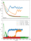 |
Fig. 12 Evolution of the semi-major axis and eccentricity of an embedded planet in discs of different masses and viscosities. The planet is inserted at a time 88 000 Tbin on a circular orbit with ap = 6 abin and held fixed for the first 2000 Tbin. |
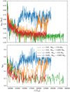 |
Fig. 13 Evolution of the semi-major axis and eccentricity of the disc’s gap for the models shown in Fig. 12. |
5 Discussion
In this section we discuss several aspects concerning the physics of the radiative disc models and the planet migration process.
5.1 Role of thermodynamics
One goal of this work is to investigate what impact the disc’s thermal structure has on its dynamical evolution. For this purpose we extended our previous locally isothermal models in Thun et al. (2017), Thun & Kley (2018) taking viscous energy dissipation into account, and assuming a cooling prescription using a vertically averaged opacity. In such a situation the thermal structure of an accretion disc is given by the viscosity coefficient (here α) as this determines the heating rate, and the mass contained in the disc as this determines the cooling rate through the density dependent opacity. Neglecting for the moment compressive heating, for example, by shocks, the temperature evolution follows from
 (19)
(19)
where Φ denotes the viscous dissipation, and Q− the cooling from Eq. (10). Taking for a simple estimate the dominant rφ-component of the stress tensor into account, the dissipation is given by Eq. (18). In the inner regions of the disc the opacity for our models varies as κ ∝ T and shows no density dependence, see Fig. 2. The viscosity varies as  (see Eq. (3)) and the sound speed is ∝ T1∕2. For the equilibrium temperature of the disc we then find, using Φ = Q−, the following dependence on mass and viscosity
 (20)
(20)
This relation explains very well the fact that the disc temperature in the four disc models displayed in Fig. 11 are very similar to each other at the edge of the central cavity. In the models with the reduced viscosity the density is higher because less mass is transferred into the cavity which would result in a higher temperature but this is compensated by the lower viscosity. In the outer regions of the discs the densities are similar and the temperature is reduced for the small viscosity models. In addition to the viscous dissipation we checked the impact of shock heating, given by the work done by compression, − P ∇⋅u. We find that this term is highly variable and only contributes near the inner rim of the central gap.
5.2 Comparison to locally isothermal models
Concerning the overall evolution of the system, one important difference between this and our previous locally isothermal models (Thun & Kley 2018) seems to be the extended initial phase before the system eventually reaches an equilibrium sate. This is most likely caused by the fact that in the full models the initial cooling in regions with lower density results in low temperatures with low pressure and small viscosity such that very large and highly eccentric cavities are produced in the early phase, as shown for example in Fig. 8. In the subsequent evolution the disc adjusts slowly on the longer viscous timescale and closes the inner disc region again. In the locally isothermal models this effect was less pronounced because the temperature, and consequently the viscosity, in the disc were always fixed and the disc did much less show this overshoot behaviour especially for high α and/or high binary eccentricities. The models for the Kepler-16 parameter show a very similar initial dynamical behaviour, as demonstrated in Figs. 4 and 5. The transient feature seen here during the initial evolution can only be a feature of real discs in case of a sudden change of the disc properties because slow variations would lead to a continuous re-adjustment. Sudden changes of the disc could occur for example by a flyby of an additional object.
On the other hand, the final equilibrium states for both cases are quite similar, when locally isothermal models are compared to radiative ones which show a similar disc height. In our previous study (Thun & Kley 2018) we constructed sequences of locally isothermal models using a fixed H∕r = 0.05 and α = 0.01 for Kepler-38 parameter. In the situation studied here, the two radiative models using the smaller disc mass (0.0057 Mbin) result in temperatures that give a H∕r value very close 0.05 in the inner disc regions for both viscosities. And indeed, the gap size and eccentricity are very compatible. In Thun & Kley (2018) we find in equilibrium for Kepler-38 values of agap = 4.5 abin and egap = 0.34, while here we obtain for the α = 0.01 model agap = 4.04 abin and egap = 0.37 (orange curves in Fig. 8). From these viscous heated simulations we can see that in isothermal simulations, a constant aspect ratio is reasonable for the inner part of a binary system up to about 15− 20 abin.
5.3 Irradiation
The models presented in this work do not include stellar irradiation. Here we justify this simplification. In the temperature panel of Fig. 11 we over-plot the expected equilibrium temperature of a disc that is heated by a single star with one solar mass. This serves as a conservative estimate for the expected irradiation because it is slightly more luminous than both binary stars together. For the inner 10 abin viscous heating is the primary heat source of the main disc. Due to the very low density within the gap viscous heating is strongly reduced and irradiation becomes more important there. Dynamically, the effects are limited because of the little mass contained in this region, but a more detailed treatment should take irradiation into account.
Beyond this radius irradiation can become more important, depending on viscosity and disc mass. As the luminosity of a star scales with stellar mass to the power of about 3.5, binary systems have a much lower luminosity for the same total mass than a single star system. Therefore, in the case of a binary, viscous heating can become more relevant than irradiation. In the outer regions of the disc irradiation, which scales with  , becomes more important and it affects the value of the aspect ratio.
 |
Fig. 14 Structure of the inner disc for the Kepler-38 system with an embedded planet for different disc parameters. The surface density is colour-coded, since the absolute density values are not important for the disc structure we omit the density scale for clarity (brighter colours mean higher surface densities). The disc structure is shown after 225 000 binary orbits. The binary components and the planets are marked with black dots. The direction of pericentre of the secondary (green), the planet (blue) and the disc (orange) are marked by the arrows. Additional fitted ellipses to the central cavity are plotted in dashed white lines and the actual orbit of the planet is shown as dashed blue line. Using the fitted ellipses, the size and eccentricity of the disc gap, shown in the upper left edge of each panel, are calculated at the same time. |
5.4 Inner disc region
Using a polar grid does not allow us to cover the central region which include the binary stars. Based on our previous studies (Thun et al. 2017), where we tested in detail the impact of the location of the inner boundary on the results, we performed all the present simulations with a value Rmin = abin. As all simulations show clear gaps with very low densities this value of Rmin should be sufficient for an accurate determination of the disc dynamics around binaries. However, this does not allow us to follow the flow of gas inside of the gap and calculate which star will accrete the material eventually.
The imposed outflow boundary at Rmin does not allow for mass flowing back into the computational domain. In reality, gas leaving through the inner boundary could come back into the domain being “flung out” by one of the binary stars. But recent simulations (Muñoz et al. 2019) show that gas entering the gap is accreted onto the stars in circumstellar discs and does not influence the ambient circumbinary disc. Hence, as the inner boundary in our model lies well within the gap it does not influence the dynamics of the circumbinary disc.
In a recent work, Mösta et al. (2019) present simulations of the inner region near the central binary in which they resolve the individual circumstellar discs covering 5000 binary orbits. In a comparison simulation using our standard setup with Rmin = abin we find very similar features in the inflow regime. This demonstrates that even in the early phases of the simulation the inner region inside a binary separation does not alter the disc behaviour and the chosen boundary condition creates an environment for the disc similar to a simulation with the full domain.
5.5 Evolution of the binary
In the simulations in which the migrating planet the central binary is also allowed to evolve due to the gravitational action of the disc. The disc torque will lead to a shrinkage of the orbit accompanied by an increase in eccentricity. Over the whole time span of the active simulations from 90 000 to 225 000 Tbin the binary semi-major axis changes only very little. The largest reduction (2.5%) is seen for the model with α = 0.01, Mdisc = 0.01 Mbin, the smallest (1.2%) for α = 0.001, Mdisc = 0.0057 Mbin. At the same time the highest increase (to 0.123) in ebin is seen for the model with α = 0.001, Mdisc = 0.01 Mbin the lowest one (to 0.103) for the α = 0.01, Mdisc = 0.01 Mbin model. These changes are so small that they have no significant impact on the evolution of the planet or disc structure, such that in future simulations of this kind the evolution of the binary can be neglected.
The mentioned test simulations in Thun et al. (2017) and the comparison to Miranda et al. (2017) and to Mösta et al. (2019) give us some confidence that by leaving out the innermost region of the binary we do not loose significant dynamics. This can only be checked in simulations where the whole domain is covered. The question of whether the binary experiences an orbit shrinkage (as due to the disc torques) or an expansion (for example due to direct accretion of high angular material from the disc) can only be studied by computations that cover the whole domain. Recent examples that find some evidence for an expansion of the binary are the simulations by Muñoz et al. (2019) or Moody et al. (2019). It remains to be seen whether this persists for discs with full thermodynamics.
5.6 Evolution of the planet
In agreement with previous studies (Pierens & Nelson 2013; Kley & Haghighipour 2014) we have shown that an embedded planet migrates to the edge of the central cavity. Additionally, we confirm the existence of two final states. In the first case (high state) the planetary orbit has a larger eccentricity (usually around ep ≈ 0.2–0.3) and is fully aligned with the eccentric hole of the disc, meaning that the planet and gap precess at the same rate. In the second case (“low state”) the orbit of the planet remains circular and the final semi-major axis is smaller than in the first case. Here, and in our previous study (Thun & Kley 2018) we demonstrate that the high state is taken for low planet masses and/or high viscosity while the low state for higher planet masses and/or low viscosity. Hence, it is linked to the ability of gap formation by the planet in the disc which depends on exactly these two parameter (Crida et al. 2006). This connection became apparent in the locally isothermal simulations in Thun & Kley (2018), where a variation of planet mass has shown that lower mass planets end up in the high state while high mass planets reach the low state. Here, we have also investigated the viscosity dependence.
Once a planet near the inner edge is able to open its own gap, the outer disc is shielded from the action of the binary, becomes more circular, and allows for a continuation of the inward migration. When the planet is not able to open a gap, its motion is dominated by the disc and its orbit remains eccentric. This close connection between disc and planet dynamics is illustrated by a direct comparison of Figs. 12 and 13. We have illustrated this behaviour for the Kepler-38 system, where the planet is more massive but it has also been seen for Kepler-16, for example in the simulations by Mutter et al. (2017a) who discussed the evolution of growing cores in discs with low viscosity α = 0.001.
6 Summary
We have performed 2D numerical simulations of viscous accretion discs around binary stars where we included viscous heating and radiative cooling. In a first study we explored, using a given binary mass ratio of qbin = 0.29 (as in Kepler-16) and an initial disc mass of 1 ∕ 100 Mbin, the impact of the binary eccentricity on the disc dynamics. In a second part we focused on the Kepler-38 system and calculated the disc structure for two different values of disc masses and viscosities. For the Kepler-38 we then followed the evolution of an embedded planet for the four models.
We find that in all cases the discs evolve towards a quasi-stationary state with an eccentric cavity that shows a slow prograde precession. The time for attaining this equilibrium can take over 100 000 binary orbits, starting from an axisymmetric initial configuration. In contrast to locally isothermal models, the inner discs cools off initially in the centre such that gaps of large size and high eccentricity are formed because of the reduced pressure and viscosity (see Figs. 4 and 8). During the subsequent evolution the disc readjusts and settles to an equilibrium state where the in the inner disc region the vertical pressure scale height is about H ∕ R = 0.04–0.05, which depends on disc mass and viscosity. Given that these values are similar to locally isothermal simulations that typically use H ∕ R = 0.05, the gap structures are comparable concerning size and eccentricity. However, in the general case, the agreement between isothermal and radiative models will depend on the used parameter of the system (disc viscosity and mass). Finally, radiative models alone will give the correct temperature in the disc, which allows to predict a realistic aspect ratio profile for further studies.
For the displayed model sequences we find a similar dependence of the gap precession rate on binary eccentricity as in locally isothermal models. Models with circular binaries produce holes with the highest eccentricity. Upon increasing ebin the gap size becomes smaller, less eccentric, and the precession period reduces until at a critical ebin = 0.16 the trend reverses. The gaps become larger and more eccentric with an increase of the precession period. Hence, this behaviour isoverall very similar to the locally isothermal models even with the same turning point (Thun & Kley 2018).
The temperature maximum of the disc lies inside of the density peak and coincides for the models with ebin > 0.1 with the maximum of the viscous dissipation rate, which is here the main heating source of the disc. Shock heating plays a role only in the very inner regions of the disc and contributes more for the binaries with small ebin. Concerning stellar irradiation, we find that for the parameters used here, it did not play a role in determining the energy balance of the disc. However, for more massive (luminous) stars and larger binary separations, this additional energy source will play a role and needs to be included.
Concerning the evolution of embedded planets we find that the planets migrate inward through the disc due the gravitational torques acting on them. They are parked near the inner edge of the disc because the positive density gradient acts as a planet trap (Masset et al. 2006). We find evidence for two different dynamical states of the final position. In the “high” state the planet resides at larger separations on an eccentric orbit which is precessing at the same rate as the gap region of the disc, in other words, the planetary orbit is always fully aligned with the disc. In the “low” state the planet remains on a circular orbit and is able to move closer to the central binary star. We have shown that it is the ability of the planet to open its own gap in the disc which separates the two states. The high state occurs for lower mass planets, or if the disc’s viscosity is too high that the planet cannot open its gap, such that its dynamics is determined by the eccentric disc. On the other hand, for higher planet masses or lower viscosity the planet opens a gap and shields the outer disc from the action of the binary. Hence, the disc remains circular and the planet can move in closer to the star keeping its circular orbit.
Our simulations show that the final position of the modelled planet lies slightly outside of the observed location of the Kepler-38 planet even for the low state result. Considering that the observed planet is on a nearly circular orbit, we can conclude that in the final phase of the planetary migration process the disc was in a low viscosity state. This most likely applies to the majority of the observed circumbinary planets as well, because they reside on orbits with very low eccentricity close to the binary (Hamers et al. 2018). This connection of final parking position of planets with the disc viscosity in circumbinary systems will allow to putconstraints on the disc viscosity via observed planetary orbits. Only in the systems Kepler-34 and Kepler-413 the planets show significant eccentricity and in both cases the numerical models show an even higher eccentricity of the final planetary orbit (Mutter et al. 2017a; Thun & Kley 2018). These systems require further investigation.
In a recent study investigating the stability of planetary orbits around binary stars it was argued that there is no pile-up of planets in circumbinary discs (Li et al. 2016) as in more than half of the Kepler systems it would be possible to place an additional planet inside of the observed one on a stable orbit (Quarles et al. 2018). Despite of this possibility of stable orbits, our results suggest that it might be difficult to place migrating planets that close due to the large disc gap opened by the binary. In this context, it would be useful to investigate the migration process of two planets in the disc and study their final locations and stability (Kley & Haghighipour 2015) and investigate the possibility of packed orbits around binaries (Kratter & Shannon 2014). In this context the recent new finding of a third planet in Kepler-47 circumbinary system (Orosz et al. 2019) will be of importance.
Acknowledgements
We acknowledge fruitful discussions with Richard Nelson. Daniel Thun and Anna Penzlin were funded by grant KL 650/26 of the German Research Foundation (DFG). Most of the numerical simulations were performed on the bwForCluster BinAC. The authors acknowledge support by the High Performance and Cloud Computing Group at the Zentrum für Datenverarbeitung of the University of Tübingen, the state of Baden-Württemberg through bwHPC and the German Research Foundation (DFG) through grant no INST 37/935-1 FUGG. All plots in this paper were made with the Python library matplotlib (Hunter 2007).
Appendix A Implementation of the cooling term
As mentioned in the numerics section we use a modified version of PLUTO 4.2 which was ported to run entirely on GPUs. The original version of PLUTO contains a very sophisticated cooling module (Teşileanu et al. 2008) which we did not implemented in the GPU version. We followed a simpler approach which will be described in this appendix.
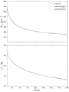 |
Fig. A.1 Equilibrium structure of a disc around a single star used as a test problem for the implementation of the cooling term. The analytical solution according to Eqs. (A.5) and (A.6) are compared, together with the results obtained using the CPU and GPU versions of the code. |
Pluto advances the hydrodynamical equations by one time step solving the following equations (we use the Runge–Kutta 2 time-step algorithm):
 (A.1)
(A.1)
 (A.2)
(A.2)
with the vector of conserved variable  and the “right-hand-side” operator
  (for details see Mignone et al. 2007). During the calculation of the right-hand-side operator, the contribution of the cooling term Δt ⋅ Q− is subtracted from the total energy of the gas.
To test our simple implementation we used the following test problem by D’Angelo et al. (2003), and simulate a Keplerian disc around a solar mass star with kinematic viscosity ν = 5 × 1016 cm2 s−1. If we assume an optical thick disc τ ≫ 1 and an opacity given by
 (A.3)
(A.3)
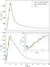 |
Fig. A.2 Direct comparison of the disc structure around the binary star for the GPU and CPU versions of the code. The CPU version uses the implementation described in Teşileanu et al. (2008). The GPU uses a simpler implementation described inthis appendix. No operator splitting means that the cooling term is directly added during the hydro step, whereas operator splitting means that after the hydro step an additional differential equation involving only the cooling term is solved (A.7) with a simple Euler method. Shown is the surface density and temperature structure after 1500 binary orbits. The inlet in the bottom panel shows a zoom in at the inner boundary of the computational domain. |
with κ0 = 2 × 10⁻⁶. The cooling term is given by
 (A.4)
(A.4)
see Eqs. (10)–(12). In such a disc the equilibrium surface density and temperature are given by
 (A.5)
(A.5)
 (A.6)
(A.6)
For details see D’Angelo et al. (2003). Figure A.1 shows the numerical result from the CPU and GPU version of the code as well as the analytical solution. In our simulation, we began with a constant surface density Σ(t = 0) = 197 g cm−2 and a constant temperature of T(t = 0) = 352 K. We see that both versions of the code reproduce the analytical equilibrium states of the surface density and temperature. Deviations at the inner and outer boundary come from the closed boundary conditions applied there.
During our circumbinary disc simulations we noticed that the temperature rises to very high values at the inner boundary of the computational domain, where the densities are very low. To examine this behaviour, we therefore computed models for the full setup, as described in Sect. 2, using different methods of solving for the cooling. The surface density and the temperature are compared after 1500 binary orbits for the GPU and CPU version of the code. The results are summarised in Fig. A.2. The blue curves in Fig. A.2 shows result from the GPU version with the cooling term implemented as described above. The inlet in the bottom panel shows the rise of the temperature at the inner boundary. The CPU version using the module from Teşileanu et al. (2008) (green curve) does not show this rise of temperature. We therefore conclude that it is a numerical artefact. To test this hypothesis we changed the implementation of the cooling term in the GPU version from the direct approach above to an operator splitting method. In this new implementation the hydrodynamical Eqs. (A.1) are solved first, without adding the cooling term. After the hydro step, the following equation is solved as a separate sub-step in the code.
 (A.7)
(A.7)
with the simple Euler method
 (A.8)
(A.8)
The cooling source term is  , with Q− given by Eq. (10).
The orange curve in Fig. A.2 shows result using this operator splitting technique. Here the temperatureremains low at the inner boundary, comparable to the CPU version which also uses an operator splitting technique. The results shown in this paper are however calculated with the direct approach described at the beginning of this appendix. Since the surface density and pressure at the inner boundary are very low. The numerically increased temperatures do not alter our results, but in the future we will use the more suitable operator splitting method.
The time step of the CPU version is more than two orders of magnitude smaller than the time step of the GPU version. This due to the complex cooling module implemented in the CPU version (Teşileanu et al. 2008). Our GPU version implements the cooling term in a much simpler way, as described in this appendix. Due to the very low time step of the CPU version, we compared the results of the two codes after just 1500 binary orbits. In cases for which the simple Euler step does lead to numerical problems, this step could be applied multiple times during one hydro time step or solved with an iterative method.
References
- Artymowicz, P., & Lubow, S. H. 1994, ApJ, 421, 651 [NASA ADS] [CrossRef] [Google Scholar]
- Crida, A., Morbidelli, A., & Masset, F. 2006, Icarus, 181, 587 [Google Scholar]
- Cuadra, J., Armitage, P. J., Alexander, R. D., & Begelman, M. C. 2009, MNRAS, 393, 1423 [NASA ADS] [CrossRef] [Google Scholar]
- D’Angelo, G., Henning, T., & Kley, W. 2003, ApJ, 599, 548 [NASA ADS] [CrossRef] [Google Scholar]
- de Val-Borro, M., Edgar, R. G., Artymowicz, P., et al. 2006, MNRAS, 370, 529 [NASA ADS] [CrossRef] [Google Scholar]
- de Val-Borro, M., Gahm, G. F., Stempels, H. C., & Pepliński, A. 2011, MNRAS, 413, 2679 [NASA ADS] [CrossRef] [Google Scholar]
- Doyle, L. R., Carter, J. A., Fabrycky, D. C., et al. 2011, Science, 333, 1602 [NASA ADS] [CrossRef] [MathSciNet] [PubMed] [Google Scholar]
- Günther, R., & Kley, W. 2002, A&A, 387, 550 [NASA ADS] [CrossRef] [EDP Sciences] [MathSciNet] [Google Scholar]
- Hamers, A. S., Cai, M. X., Roa, J., & Leigh, N. 2018, MNRAS, 480, 3800 [NASA ADS] [CrossRef] [Google Scholar]
- Hanawa, T., Ochi, Y., & Ando, K. 2010, ApJ, 708, 485 [NASA ADS] [CrossRef] [Google Scholar]
- Hubeny, I. 1990, ApJ, 351, 632 [NASA ADS] [CrossRef] [Google Scholar]
- Hunter, J. D. 2007, Comput. Sci. Eng., 9, 90 [NASA ADS] [CrossRef] [Google Scholar]
- Kley, W. 1999, MNRAS, 303, 696 [NASA ADS] [CrossRef] [Google Scholar]
- Kley, W., & Haghighipour, N. 2014, A&A, 564, A72 [NASA ADS] [CrossRef] [EDP Sciences] [Google Scholar]
- Kley, W., & Haghighipour, N. 2015, A&A, 581, A20 [NASA ADS] [CrossRef] [EDP Sciences] [Google Scholar]
- Kratter, K. M., & Shannon, A. 2014, MNRAS, 437, 3727 [NASA ADS] [CrossRef] [Google Scholar]
- Li, G., Holman, M. J., & Tao, M. 2016, ApJ, 831, 96 [NASA ADS] [CrossRef] [Google Scholar]
- Lin, D. N. C., & Papaloizou, J. 1985, Protostars and Planets II (Tucson: University of Arizona Press), 981 [Google Scholar]
- MacFadyen, A. I., & Milosavljević, M. 2008, ApJ, 672, 83 [Google Scholar]
- Masset, F. S. 2002, A&A, 387, 605 [NASA ADS] [CrossRef] [EDP Sciences] [Google Scholar]
- Masset, F. S., Morbidelli, A., Crida, A., & Ferreira, J. 2006, ApJ, 642, 478 [NASA ADS] [CrossRef] [Google Scholar]
- Mignone, A., Bodo, G., Massaglia, S., et al. 2007, ApJS, 170, 228 [Google Scholar]
- Miranda, R., Muñoz, D. J., & Lai, D. 2017, MNRAS, 466, 1170 [NASA ADS] [CrossRef] [Google Scholar]
- Moody, M. S. L., Shi, J.-M., & Stone, J. M. 2019, ApJ, 875, 66 [NASA ADS] [CrossRef] [Google Scholar]
- Mösta, P., Taam, R. E., & Duffell, P. C. 2019, ApJ, 875, L21 [NASA ADS] [CrossRef] [Google Scholar]
- Muñoz, D. J., Miranda, R., & Lai, D. 2019, ApJ, 871, 84 [NASA ADS] [CrossRef] [Google Scholar]
- Müller, T. W. A., & Kley, W. 2012, A&A, 539, A18 [NASA ADS] [CrossRef] [EDP Sciences] [Google Scholar]
- Müller, T. W. A., Kley, W., & Meru, F. 2012, A&A, 541, A123 [NASA ADS] [CrossRef] [EDP Sciences] [Google Scholar]
- Mutter, M. M., Pierens, A., & Nelson, R. P. 2017a, MNRAS, 469, 4504 [NASA ADS] [CrossRef] [Google Scholar]
- Mutter, M. M., Pierens, A., & Nelson, R. P. 2017b, MNRAS, 465, 4735 [NASA ADS] [CrossRef] [Google Scholar]
- Orosz, J. A., Welsh, W. F., Carter, J. A., et al. 2012, ApJ, 758, 87 [NASA ADS] [CrossRef] [Google Scholar]
- Orosz, J. A., Welsh, W. F., Haghighipour, N., et al. 2019, AJ, 157, 174 [NASA ADS] [CrossRef] [Google Scholar]
- Pierens, A., & Nelson, R. P. 2007, A&A, 472, 993 [NASA ADS] [CrossRef] [EDP Sciences] [Google Scholar]
- Pierens, A., & Nelson, R. P. 2008, A&A, 483, 633 [NASA ADS] [CrossRef] [EDP Sciences] [Google Scholar]
- Pierens, A., & Nelson, R. P. 2013, A&A, 556, A134 [NASA ADS] [CrossRef] [EDP Sciences] [Google Scholar]
- Quarles, B., Satyal, S., Kostov, V., Kaib, N., & Haghighipour, N. 2018, ApJ, 856, 150 [NASA ADS] [CrossRef] [Google Scholar]
- Shakura, N. I., & Sunyaev, R. A. 1973, A&A, 24, 337 [NASA ADS] [Google Scholar]
- Teşileanu, O., Mignone, A., & Massaglia, S. 2008, A&A, 488, 429 [NASA ADS] [CrossRef] [EDP Sciences] [Google Scholar]
- Thun, D., & Kley, W. 2018, A&A, 616, A47 [NASA ADS] [CrossRef] [EDP Sciences] [Google Scholar]
- Thun, D., Kley, W., & Picogna, G. 2017, A&A, 604, A102 [NASA ADS] [CrossRef] [EDP Sciences] [Google Scholar]
All Tables
Orbital parameter of the stellar binaries in the Kepler-16 and Kepler-38 systems.
All Figures
|
Fig. 1 Sketch of our disc model with the averaging process indicated for the three-dimensional density ϱ. The orange circle marks the primary and the red circle the secondary star for the Kepler-38 system, where the sizes are proportionalto the stellar masses. The origin of the coordinate system lies at the barycentre of the binary. |
| In the text | |
|
Fig. 2 Variation of the Rosseland mean opacity with temperature for three different densities ϱ. |
| In the text | |
|
Fig. 3 Time evolution of the disc eccentricity and mass for fixed qbin = 0.29 (as in Kepler-16) and various binary eccentricities over time. Top panel: disc eccentricity. Bottom panel: total mass in the disc in units of the central binary mass. |
| In the text | |
|
Fig. 4 Evolution of the gap properties for fixed qbin = 0.29 and various binary eccentricities. Top panel: precession period of the gap as a function of period number. Bottom two panels: semi-major axis and eccentricity of the gap. The horizontal lines and labels indicate the final values. |
| In the text | |
|
Fig. 5 Azimuthally averaged radial disc profiles for ebin = 0.16 at various evolutionary times. Displayed are the surface density, the midplane temperature, the disc thickness, and the disc eccentricity. |
| In the text | |
|
Fig. 6 Azimuthally averaged radial disc profiles in equilibrium for different ebin after 180 000 binary orbits. Displayed are the surface density, the midplane temperature, the disc thickness, the disc eccentricity, and in code units the dissipation function (18). |
| In the text | |
|
Fig. 7 Gap precession period against gap size in equilibrium after 180 000 binary orbits. All the models have the same qbin = 0.29 and differentebin as indicated by the labels. |
| In the text | |
|
Fig. 8 Precession period, semi-major axis, and eccentricity of the disc gap vs. time, for discs with two different disc masses and viscosities. For the central binary we used the parameter of Kepler-38. The horizontal lines indicate time averages starting at 120 000 binary orbits, the time when all discs reached a quasi-steady state. |
| In the text | |
|
Fig. 9 Disc mass a function of time for models with different viscosity and disc mass. |
| In the text | |
|
Fig. 10 Two-dimensional density distribution of the inner disc region at a time t = 88 000. The dashed white lines and labels correspond to the approximate sizes and shapes of the inner holes. The green arrow points towards the peri-centre of the binary and the orange arrow towards the pericentre of the inner gap. |
| In the text | |
|
Fig. 11 Azimuthally averaged radial disc profiles for the different models of the Kepler-38 like system after 120 000 binary orbits. Displayed are the surface density, the midplane temperature, the disc thickness and the disc eccentricity. The black dotted line in the second panel represents the irradiation temperature of a sun-like star. |
| In the text | |
|
Fig. 12 Evolution of the semi-major axis and eccentricity of an embedded planet in discs of different masses and viscosities. The planet is inserted at a time 88 000 Tbin on a circular orbit with ap = 6 abin and held fixed for the first 2000 Tbin. |
| In the text | |
|
Fig. 13 Evolution of the semi-major axis and eccentricity of the disc’s gap for the models shown in Fig. 12. |
| In the text | |
|
Fig. 14 Structure of the inner disc for the Kepler-38 system with an embedded planet for different disc parameters. The surface density is colour-coded, since the absolute density values are not important for the disc structure we omit the density scale for clarity (brighter colours mean higher surface densities). The disc structure is shown after 225 000 binary orbits. The binary components and the planets are marked with black dots. The direction of pericentre of the secondary (green), the planet (blue) and the disc (orange) are marked by the arrows. Additional fitted ellipses to the central cavity are plotted in dashed white lines and the actual orbit of the planet is shown as dashed blue line. Using the fitted ellipses, the size and eccentricity of the disc gap, shown in the upper left edge of each panel, are calculated at the same time. |
| In the text | |
|
Fig. A.1 Equilibrium structure of a disc around a single star used as a test problem for the implementation of the cooling term. The analytical solution according to Eqs. (A.5) and (A.6) are compared, together with the results obtained using the CPU and GPU versions of the code. |
| In the text | |
|
Fig. A.2 Direct comparison of the disc structure around the binary star for the GPU and CPU versions of the code. The CPU version uses the implementation described in Teşileanu et al. (2008). The GPU uses a simpler implementation described inthis appendix. No operator splitting means that the cooling term is directly added during the hydro step, whereas operator splitting means that after the hydro step an additional differential equation involving only the cooling term is solved (A.7) with a simple Euler method. Shown is the surface density and temperature structure after 1500 binary orbits. The inlet in the bottom panel shows a zoom in at the inner boundary of the computational domain. |
| In the text | |
Current usage metrics show cumulative count of Article Views (full-text article views including HTML views, PDF and ePub downloads, according to the available data) and Abstracts Views on Vision4Press platform.
Data correspond to usage on the plateform after 2015. The current usage metrics is available 48-96 hours after online publication and is updated daily on week days.
Initial download of the metrics may take a while.