| Issue |
A&A
Volume 627, July 2019
|
|
|---|---|---|
| Article Number | A62 | |
| Number of page(s) | 10 | |
| Section | The Sun | |
| DOI | https://doi.org/10.1051/0004-6361/201935357 | |
| Published online | 02 July 2019 | |
Exploring the damping of Alfvén waves along a long off-limb coronal loop, up to 1.4 R⊙
1
DAMTP, Centre for Mathematical Sciences, University of Cambridge, Wilberforce Road, Cambridge CB3 0WA, UK
2
Udaipur Solar Observatory, Physical Research Laboratory, Badi Road, Udaipur 313 001, India
e-mail: This email address is being protected from spambots. You need JavaScript enabled to view it.
Received:
25
February
2019
Accepted:
23
May
2019
Abstract
The Alfvén wave energy flux in the corona can be explored using the electron density and velocity amplitude of the waves. The velocity amplitude of Alfvén waves can be obtained from the non-thermal velocity of spectral line profiles. Previous calculations of the Alfvén wave energy flux with height in active regions and polar coronal holes have provided evidence for the damping of Alfvén waves with height. We present off-limb Hinode Extreme-ultraviolet Imaging Spectrometer (EIS) observations of a long coronal loop up to 1.4 R⊙. We obtained the electron density along the loop and found the loop to be almost in hydrostatic equilibrium. We obtained the temperature using the emission measure-loci (EM-loci) method and found the loop to be isothermal across, as well as along, the loop with a temperature of about 1.37 MK. We significantly improve the estimate of non-thermal velocities over previous studies by using the estimated ion (equal to electron) temperature. Estimates of electron densities are improved using the significant updates of the CHIANTI v.8 atomic data. More accurate measurements of propagating Alfvén wave energy along the coronal loop and its damping are presented up to distances of 1.4 R⊙, further than have been previously explored. The Alfvén wave energy flux obtained could contribute to a significant part of the coronal losses due to radiation along the loop.
Key words: Sun: corona / Sun: UV radiation / waves / turbulence
© ESO 2019
1. Introduction
The definitive physical processes responsible for the heating of solar corona and acceleration of solar wind have not yet been identified. There are several theories which exist to explain phenomena such as wave dissipation (AC) models, foot-point stressing (DC) models, turbulence models, and Taylor relaxation models (see recent review by Cranmer & Winebarger 2019). Coronal loops are the basic building blocks of the solar corona. Priest et al. (1998) found that physical parameters such as the temperature profile along the coronal loop are highly sensitive to heating mechanisms. Thus, to distinguish among the different heating models, accurate measurements of basic plasma parameters along the coronal loops, such as temperature, density, filling factor, velocity, non-thermal velocity, and magnetic field are essential (e.g. Gupta et al. 2015; Xie et al. 2017). Several observational studies of loop characteristics, such as the derivation of temperatures and densities, have been published (see e.g. Del Zanna & Mason 2003; Landi & Landini 2004; Aschwanden et al. 2008; Tripathi et al. 2009; Lee et al. 2014; Ghosh et al. 2017). More details can be found in recent review by Del Zanna & Mason (2018).
In the wave dissipation model of the solar atmosphere convective motions at the magnetic foot-points of the loop are assumed to generate wave-like fluctuations. This wave energy is then transmitted up into the corona, where the conversion to heat can occur (e.g. Cranmer et al. 2007; Van Ballegooijen et al. 2011). Among the different types of waves, Alfvén waves are the least damped during propagation to the chromosphere and carry sufficient energy to heat the solar corona (see reviews by De Moortel & Nakariakov 2012; Mathioudakis et al. 2013).
However, in the corona, several spatially unresolved structures may be present along the line of sight. These unresolved structures may be oscillating with different phases and could lead to excess broadening of spectral line profiles. Spectroscopic observations of coronal loops have clearly shown that the line widths of observed emission lines are significantly broadened in excess of their corresponding thermal widths (e.g. Doschek et al. 2007; Doschek 2012; Lee et al. 2014; Asgari-Targhi et al. 2014; Brooks & Warren 2016; Testa et al. 2016; Gupta 2017; Xie et al. 2017). These observed non-thermal broadenings of spectral line profiles in the corona are expected to be proportional to Alfvén wave amplitudes (e.g. Hassler et al. 1990; Doyle et al. 1998; Banerjee et al. 1998; Moran 2001). Thus, upon comparison of non-thermal velocity estimates with height, we can infer the variation of Alfvén wave amplitude with height. Using such measurements, evidence of the damping of Alfvén waves has been reported along the coronal loops (Lee et al. 2014; Gupta 2017).
In this paper, our main focus is on the estimation of electron density, temperature, plasma filling factor, and non-thermal velocity along the coronal loop, up to a very large distance. Further, we aim to obtain the total Alfvén wave energy flux along the loop so as to find any signatures of Alfvén wave damping. For this purpose, we identified a unique set of spectroscopic data covering a very large distance in the off-limb active and quiet Sun regions observed by Extreme-ultraviolet Imaging Spectrometer (EIS; Culhane et al. 2007) on board Hinode (Kosugi et al. 2007). Details of the observations are described in Sect. 2. We employ several spectroscopic methods, which are described in Sect. 3 to obtain the electron number density, temperature, plasma filling factor, effective and non-thermal velocity, and to derive the Alfvén wave energy flux. The results obtained are discussed and summarised in Sect. 4.
2. Observations and data analysis
Because of the constraints on Hinode pointing outside the solar limb, off-limb observations of coronal loops reaching far out in the corona using EIS are very rare with the exception of several observations reaching far out in the polar regions. In order to overcome this issue and to reach greater distances, one of us (GDZ) designed an EIS engineering study (study ID 141) to extract spectra from the bottom half of the long EIS slit. The Joint Hinode Observational Program (Hinode HOP 7) was coordinated to obtain simultaneous SOHO/Hinode/TRACE/STEREO observations during May 7–10 2007. The HOP was summarised in Del Zanna et al. (2009) and some results from other days of the campaign are presented in Del Zanna et al. (2018a,b). On May 9, a long coronal loop appeared on the west limb. The region was rastered by the EIS 2″ slit with an exposure time of 60 s. The EIS slit moved with an 8″ step size and a total of 60 exposures were taken, which covered the total field of view of 480″ × 512″. We selected the raster which began on that day at 14.25.12 UT for a detailed analysis. We binned the data over four pixels along the slit to improve the signal-to-noise ratio. We followed the standard solar software (SSW) procedure EIS_PREP for preparing the EIS data. All the EIS spectral line profiles were fitted with a Gaussian function using EIS_AUTO_FIT (Young 2015). The routine also provides 1σ error bars on the fitted parameters. The EIS sensitivity is degrading with time, therefore we further recalibrated the intensities and related errors using the method of Del Zanna (2013). We assumed the instrumental profile to be Gaussian and subtracted the instrumental width following the method described in Young (2011). Moreover, our analyses (Del Zanna et al. 2018b) of variation of instrumental width along the slit also show similar results of 65–72 mÅ, which is within a few mÅ of Young (2011). Spatial offsets in the solar-X and solar-Y directions between images obtained from different wavelengths were corrected with respect to the image obtained from the Fe XII 195.12 Å spectral line.
In Fig. 1, we plot monochromatic intensity maps of the off-limb region obtained from Fe X 184.54, Fe XI 188.23, Fe XII 195, and Si X 258 Å spectral lines. Images obtained from these lines show the presence of a clear coronal loop extending very far off-limb. In the images from other spectral lines, the loop is more difficult to discern. In Fig. 2, we also show the STEREO-B EUVI images taken in 195 Å passband at different times overlapping the time interval of EIS raster scan. During this interval, STEREO-B was just 2.3° ahead of the Sun-Earth line in the ecliptic plane, thus viewing almost same part of the Sun. Images obtained at different times show the clear presence of two long loops reaching far out. The loop at the bottom shows dynamic motion, whereas the upper loop is relatively stable. Thus, we focus our attention on studying the upper loop.
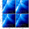 |
Fig. 1. Intensity maps obtained from Fe X 184.54, Fe XI 188.23, Fe XII 195, and Si X 258 Å showing clear long loops in all the panels. |
 |
Fig. 2. Intensity maps obtained from the STEREO-B EUVI 195 Å passband showing clear long loops at different times as labelled. |
We calculated the contribution function of the EIS spectral lines chosen for this study using CHIANTI v.8 (Dere et al. 1997; Del Zanna et al. 2015) at a constant electron number density Ne = 108 cm−3. The peak formation temperatures of all the selected lines are labelled in Fig. 1. We also identified density-sensitive lines Fe XII 186.88 and Si X 258.37 Å and used these for the purpose of deriving electron number densities along the loop length.
In Fig. 3, we plot monochromatic intensity maps of the off-limb active region obtained from Fe XII 195.12 Å. We trace the loop using this image. The traced points are indicated with asterisks (*). We also identified a quiet region near the loop for the background/foreground subtraction purposes (also marked with asterisks). We created a curved box along the loop to study the loop parameters. The curved box is shown with a white continuous line.
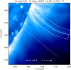 |
Fig. 3. Intensity maps obtained from Fe XII 195 Å showing the loop traced out to study in detail. The quiet Sun region is also traced out for the purpose of determining the background. The white curved box indicates region chosen along the curved loop. |
From the curved box, we obtained an intensity across the loop at each of the traced points using the image from the Fe XII 193 Å line. We fitted these intensity profiles across the loop positions with a Gaussian function. The full width half maximum (FWHM) of the Gaussian profile provides a geometric width of the loop at that position. We obtained the height of the loop with respect to the solar limb. We also summed individual segments of the loop to obtain the length of the loop. The loop length and width obtained are plotted in the top and bottom panels of Fig. 4, respectively. The figure clearly shows that the loop is traced up to the height of 270 Mm and has a total length more than 280 Mm. This also indicates that actual length and height of the loop would have been even longer and likely went beyond the EIS field of view (FOV). The geometric width of the loop increases with height from 20 Mm near limb to nearly 80 Mm at the distance of 1.37 R⊙.
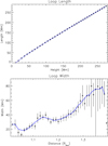 |
Fig. 4. Length (top panel) and width (bottom panel) of the long coronal loop with distance as obtained from the Fe XII 193 Å intensity map. |
3. Results
We obtained the various parameters along the loop such as intensity, density, temperature, plasma filling factor, and Alfvén wave energy flux. We describe the estimation of all these parameters in the following subsections.
3.1. Intensity
In Fig. 5, we plot the intensities obtained along the loop and quiet Sun region with height. The 1σ error bars associated with the data points are overplotted. It is clear from the plots that the spectral lines have a good enough signal to perform a further detailed analysis.
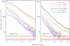 |
Fig. 5. Intensity obtained from Fe X 184.54, Fe XII 186.88*, Fe XI 188.23, Fe XII 195.12, and Si X 258.37*, 261.04 Å spectral lines along the coronal loop (left panel) and quiet Sun region (right panel) with height. The intensities are recalibrated using the method of Del Zanna (2013). The asterisks denote respective spectral lines are density sensitive. Horizontal lines denote expected level of scattered light as per Ugarte (2010). |
We also estimated the level of scattered light in the intensities using available field of view of on-disc region as suggested by Ugarte (2010), which is expected to be about 2% of the disc intensity. This level is also overplotted in the Fig. 5 for all respective spectral lines. However, scattered light estimate of Hahn et al. (2012) indicates that a 2% level of scattered light contribution is an overestimation in the polar coronal hole region. Del Zanna et al. (2018a) analysed the same type of observation as performed in this work on the May 10 (one day after). Their analysis indicates that scattered light usually assumed at 2% level is an overestimate even up to 1.3 R⊙. Therefore, it is safe to assume that scattered light contribution in the coronal loop is negligible as structure is visible until the end of EIS FOV, thus can conveniently be ignored in the further analysis.
We also obtained the variation of intensity ratios of Fe XII 193.51 and 195.12 Å lines along the loop and plot these in Fig. 6. From the CHIANTI database, this ratio is expected to be constant at 0.67 without any variation with height. However, recently Del Zanna et al. (2018b) reported the Fe XII 193.51 and 195.12 Å intensity ratios to be different from the expected theoretical value where the deviation is about 30−40% in the quiet and active regions. These authors speculated the cause for these anomalies to be either an opacity effect or some non-linear behaviour in the CCD counts. However, in our observation, the variation in the intensity ratio is relatively small (< 10%).
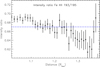 |
Fig. 6. Measured intensity ratios of Fe XII 193.51 and 195.12 Å lines along the coronal loop. This ratio is expected to be constant at 0.67 as per CHIANTI v.8 database (dashed line). |
3.2. Electron density along the coronal loop
We estimated the electron number density along the loop using the line ratio method (see recent review by Del Zanna & Mason 2018). For the purpose, we identified the density sensitive line pairs of Fe XII λ186.88/λ195.12 and Si X λ258.37/λ261.04. In Fig. 7, we plot densities obtained from both the line pairs. We also obtained these densities after subtracting the background as identified from the quiet region. The densities obtained from the background subtracted intensities are relatively higher than those obtained without background subtraction (BS). A closer inspection indicates that densities obtained with BS have higher values compared to densities obtained without BS only near the limb, whereas in the far off-limb region both the densities have almost the same values. This is because the background signal is present only near the limb region and in far off-limb region, there is hardly any background signal. Also, there are huge error bars on the densities obtained from the Si X λ258.37/λ261.04 line pair. Electron number densities along the loop as obtained from Fe XII λ186.88/λ195.12 show the number density to be around 109 cm−3 near the limb, which falls to ≈107.9 cm−3 at a far off-limb distance.
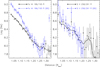 |
Fig. 7. Electron density obtained from the Fe XII line ratio method with (dashed lines) and without (solid lines) BS, as labelled. |
3.3. Electron temperature along coronal loop
The electron temperature of the plasma can be estimated using emission lines from ions of different ionisation stages. Since contribution functions of spectral lines are highly temperature dependent, the observed intensity can be converted in to temperature by analysing different ions. We used the technique of the emission measure-loci (EM-loci) method to estimate the temperature along the coronal loop (e.g. Del Zanna et al. 2002). In this method, EM curves obtained from different ions are plotted as a function of temperature. If the emitting region is isothermal then all of the curves would cross at a single location, thus, indicate a single temperature. We used density insensitive emission lines Fe X 184.54, Fe XI 188.23, Fe XII 193.51, and Si X 261.04 Å to obtain EM-loci curves. Thus, we obtained EM-loci curves at all locations along the loop to obtain electron temperatures along the loop (see e.g. Gupta et al. 2015). In Fig. 8, we show EM curves obtained only at distance of 1.10, 1.15, 1.20, and 1.25 R⊙. All the EM curves cross at almost the same temperature at all locations, suggesting that the loop is nearly isothermal along and across its length. However, there is a slight difference in temperature crossing points among different lines. Thus, we choose an average temperature at crossing points as the electron temperature and standard deviation of temperatures at crossing points as standard error bars on the electron temperatures. However, there also exist uncertainties in the atomic data which are utilised in the CHIANTI database. Although, it is difficult to quantify uncertainties present in various atomic data, in this work we assume a total of about 15% uncertainties present in the contribution function of spectral lines. Therefore for error estimation, we assumed 15% errors on EMs and associated temperature. Using this we again calculated larger error bars on the temperature along the loop. In Fig. 9, we plot electron temperatures obtained along the loop. Error bars obtained from standard deviation of temperatures at crossing points are plotted in magenta (small error bars), whereas cummulative error bars obtained after taking in to account all the errors are plotted in black (large error bars). The figure indicates that the temperature obtained from the EM-loci method is almost constant along the loop within the smaller error bars. However, a slight increase in the temperature is also observed at the far distances.
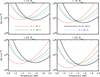 |
Fig. 8. Emission measure (EM) loci curves obtained from Fe X 184.54, Fe XI 188.23, Fe XII 193.51, and Si X 261.04 Å spectral lines at different heights as labelled. |
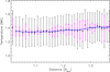 |
Fig. 9. Temperature obtained along the coronal loop as obtained from the EM-loci curves. |
3.4. Comparison with hydrostatic equilibrium
We fitted the electron number density variation with height along the loop with an exponential function Ne = N0exp(−h/Hd) using MPFIT routines (Markwardt 2009). The fit provides the density scale height Hd along the coronal loop. For this purpose, we chose only the Fe XII line pair as density measurements from Si X line pair show relatively larger error bars and are more noisy. We fitted both the density profiles obtained from Fe XII line pair with and without BS. Fitted profiles to density variations are plotted in Fig. 10. The fit resulted in density scale heights of 59 ± 3 and 81 ± 3 Mm for density profiles with and without background subtracted, respectively.
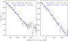 |
Fig. 10. Electron densities obtained from the line pair of Fe XII λ186.88/λ195.12 with and without BS plotted in right and left panels, respectively. Densities are fitted with an exponential function to obtain the density scale height which are also printed on the figures. |
Recalling that the background subtracted densities are larger near the limb compared to without background subtracted densities, whereas both are almost the same in the far off-limb region. This indicates a rapid fall of density in the background subtracted measurements, and thus gives the smaller density scale height as compare to without background subtracted measurements. Density scale heights obtained from the fits are also labelled in the Fig. 10.
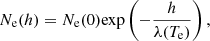
Electron number densities obtained along the loop can be compared with the hydrostatic equilibrium model (e.g. Aschwanden et al. 1999; Gupta et al. 2015). Electron number density profile in hydrostatic equilibrium is given by
 (1)
(1)
where λ is the density scale height given by
![Mathematical equation: $$ \begin{aligned} \lambda (T_{\rm e})= \frac{k_{\rm B} T_{\rm e}}{\mu m_{\rm H} g} \approx 46 \left[ \frac{T_{\rm e}}{1\,\mathrm{MK}} \right] [Mm], \end{aligned} $$](/articles/aa/full_html/2019/07/aa35357-19/aa35357-19-eq2.gif) (2)
(2)
where kB is the Boltzmann constant, Te is electron temperature, μ is mean molecular weight (≈0.7 for the solar corona), mH is mass of the hydrogen atom, and g is acceleration due to gravity at the solar surface (see e.g. Aschwanden et al. 1999).
The density scale height for hydrostatic equilibrium is calculated to be ≈63 Mm for an electron temperature of 1.37 MK as obtained from the EM-loci method. The observed density scale heights are 59 ± 3 and 81 ± 3 Mm for with and without background subtracted density profiles, respectively. These are reasonably close to the hydrostatic equilibrium height.
We also calculated coronal plasma filling factor, which is defined as the ratio of the volume emitting plasma contributing to the EUV emission lines to the total volume observed. This parameter provides information on whether the observed coronal structures are resolved or unresolved with the given instrument, using the formula  , where EM is obtained in Sect. 3.3, Ne is measured in Sect. 3.2, and h is column depth, which is assumed to be width of the loop measured in Sect. 2. The obtained plasma filling factors along the loop are plotted in Fig. 11. Error bars on filling factors were obtained following standard procedures, which include errors on Ne, EM, and loop width (1σ error on FWHM of geometric profile of loop). Near the limb, filling factors are less than unity and increase with height as obtained in previous measurements (e.g. Tripathi et al. 2009). At some distance, the filling factor becomes more than unity, which is unrealistic. One interpretation is that we could be seeing an arcade of loops, where the distance along the line of sight is greater than the measured geometric width.
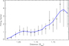 |
Fig. 11. Plasma filling factor obtained along the coronal loop. |
3.5. Effective and non-thermal velocity
The observed FWHM of any coronal spectral line is given by
![Mathematical equation: $$ \begin{aligned} FWHM = \left[4 \mathrm{ln} 2 \left(\frac{\lambda }{c}\right)^2 \left(\frac{2 k_{\rm B} T_{\rm i}}{M_{\rm i}} +{\xi }^2\right) + W^{2}_{\rm inst}\right]^{1/2} ,\end{aligned} $$](/articles/aa/full_html/2019/07/aa35357-19/aa35357-19-eq4.gif) (3)
(3)
where Ti is ion temperature, Mi is ion mass, ξ is non-thermal velocity, and Winst is the instrumental width.
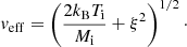
After subtracting the instrumental width, the observed intrinsic line width of solar origin can then be expressed as an effective width and velocity veff (e.g. Hara et al. 2011),
 (4)
(4)
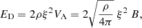
Thus, veff mainly depends upon Ti and ξ. Upon assuming plasma to be in thermal equilibrium, Ti can be approximated as Te (i.e. Ti ≈ Te), where Te is obtained in Sect. 3.3. Ti = Te is a common valid assumption which may not be true for coronal holes. We do not expect any large departures in this assumption for this relatively quiescent loop, at least in the main part of the loop. As an order of magnitude for a Fe XII ion, using the CHIANTI recombination rates and the measured electron densities, the recombination time near the limb turns out to be about 5 s, while at the lower density of 108 cm−3 the value becomes almost 1 min, which significantly validates our assumption. In Fig. 12, we plot the effective velocity obtained from Fe X 184.54, Fe XI 188.23, Fe XII 193.51, and Si X 258.37 Å spectral lines. Fe XII 193.51 Å, which is the strongest line, shows an almost constant effective velocity with height. Other lines show a large scatter in data points in the far off-limb region but give a hint of slight increase in the velocity up to 1.3 R⊙.
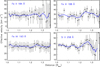 |
Fig. 12. Effective velocity (combined thermal and non-thermal velocity) obtained along the coronal loop from various spectral lines as labelled. |
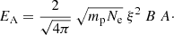
In Fig. 13, we plot the non-thermal velocities (ξ) obtained from Fe X 184.54, Fe XI 188.23, Fe XII 193.51, and Si X 258.37 Å spectral lines. For this purpose, we incorporated electron temperature Te obtained in Sect. 3.3 to calculate the thermal velocity. Again Fe XII 193.51 Å, the strongest line, shows almost constant non-thermal velocity with height. Other lines show some increasing trend in the non-thermal velocity with height, however, the data points are highly scattered. The average non-thermal velocity, as obtained from Fe XII 193.51 Å is ≈23 km s−1. Si X 258.37 Å shows an average value of ≈30 km s−1 with some increase with height. However, non-thermal velocities from Fe X 184.54, and Fe XI 188.23 Å show relatively lower values. Interestingly, Del Zanna et al. (2018b) have noted that the instrumental width for Fe XII 193.5 Å line appears to be constantly larger than that of the other lines. They also noticed the overestimation in line widths from Fe XII 193.51 Å line, which is partly due to instrumental issues and partly due to opacity effects in the stronger lines of Fe XII based on line ratio of Fe XII λ193.51/λ195.12. However, in our coronal loop, deviation of line ratio is within 10% (see Fig. 6). Thus, non-thermal velocity estimation from Fe XII 193.51 Å is mildly affected.
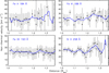 |
Fig. 13. Non-thermal velocity obtained along the coronal loop from various spectral lines as labelled. |
3.6. Alfvén wave energy flux
The Alfvén wave energy flux density is given by
 (5)
(5)
where ρ is mass density (ρ = mpNe, mp is proton mass, and Ne is electron number density), ξ is Alfvén wave velocity amplitude, 2 for two degrees of freedom, and VA is Alfvén wave propagation velocity given as  . Therefore, the total Alfvén wave energy crossing a surface area A per unit time is given by
 (6)
(6)
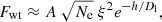
Henceforth, the total Alfvén wave energy propagating along the loop depends on the electron number density, wave amplitude, magnetic field, and area of cross section. However, the product of magnetic field B and cross-section area A is always a constant along the loop owing to magnetic flux conservation. Therefore, the total Alfvén wave energy propagating along the loop is always proportional to  . The product of
  is expected to be constant with height if the total Alfvén wave energy is conserved as wave propagates along the loop. Thus, we obtain the proportional Alfvén wave energy (
 ) along the loop using the Ne (see Sect. 3.2) and ξ (see Sect. 3.5) obtained from Fe XII spectral lines. In Fig. 14, we plot variations of
  with height. The plot shows that
  decreases with height. Thus this provides evidence of damping of Alfvén wave energy with height along the coronal loop, although associated error bars are very large on individual data points.
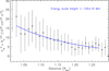 |
Fig. 14. Proportional Alfvén wave energy ( |

We further obtain the damping length using the equation (e.g. Gupta 2017)
 (7)
(7)
where Dl is “damping length” for the decay of total Alfvén wave energy with height, and A is appropriate constant. Upon fitting with MPFIT routines (Markwardt 2009), we found the damping length to be 126 ± 19 Mm. The damping length obtained by Gupta (2017) using Fe XII 192.39 Å was also of the same order in the active region. Thus, both the results are in good agreement.
4. Discussion and summary
In this work, we presented the estimation of various plasma parameters along the long coronal loop using the EIS spectroscopic data. Spectroscopic diagnostics were used to measure electron density, temperature, non-thermal velocity, and thus Alfvén wave energy flux along the loop length. The loop was clearly visible in the EIS Fe X 184.54, Fe XI 188.23, Fe XII 193.51, and Si X 258.37 Å spectral lines covering the peak formation temperature of 1.1−1.6 MK. The cross section (geometric width) of the loop increases with height. The observed width is about 20 Mm near the limb which increases up to 80 Mm at the distance of 1.37 R⊙. Increase in the loop cross section with height is also seen in the Gupta et al. (2015). However, most of the coronal loops have been found to show roughly constant cross section or slight increase in cross section with height (e.g. Watko & Klimchuk 2000). It is interesting to note that no systematic study exists on the cross-section variation of fan loops with height.
We obtained the electron density along the loop reaching far off-limb distance. Densities were obtained using the density sensitive EIS spectral line pairs Fe XII λ186.88/λ195.12 and Si X λ258.37/λ261.04. Obtained number densities are around 109 cm−3 near the limb, which falls to ≈107.9 cm−3 at far off-limb distances. Del Zanna & Mason (2003) also obtained the electron densities along the off-limb coronal loops and found a high density ≈3 × 109 cm−3 near the base and rapid fall with height. We also compared the fall in density with the hydrostatic equilibrium model, which indicates that the loop is almost in hydrostatic equilibrium. Obtained with and without BS, density scale heights are 59 ± 3 and 81 ± 3 Mm, respectively, which are close to the hydrostatic scale height of 63 Mm. Lee et al. (2014) also studied the cool loops in off-limb region and found density scale heights in the range 60−70 Mm from the Fe XII λ186.88/λ195.12 line pair. Interestingly, Winebarger et al. (2003) found long, cool loops to be overdense whereas short hot loops to be underdense on comparison with the static solutions. However, the existence of such loops may be explained by impulsive heating models (e.g. Klimchuk et al. 2008).
We used the EM-loci technique to estimate electron temperature along the coronal loop. Results obtained clearly show that plasma along the line of sight in the loop is isothermal as all the EM curves cross at a single point. The result also indicates that the temperature along the loop is also constant (within the obtained error bars). Thus, the observed loop is isothermal across and along the loop with a temperature around ≈1.37 MK. Tripathi et al. (2009) also studied the long coronal loop, however on-disc, and found the loop to be nearly isothermal along the line of sight. However, these authors noted that temperature along the loop increases from 0.8 MK near the base to 1.5 MK at the height of 75 Mm.
We estimated the effective and non-thermal velocities along the coronal loop length. The strongest line Fe XII 193.51 Å shows an almost constant effective and non-thermal velocity with height. Other lines show a somewhat increasing trend with height, however, there is large scatter present in the data points. The non-thermal velocity obtained from Fe XII 193.51 Å line is around 23 km s−1. Gupta (2017) found an increase in non-thermal velocity from ≈24 km s−1 near the limb to ≈33 km s−1 around the height of 80 Mm along the coronal loop from Fe XII 192.39 Å line. However, Lee et al. (2014) found decrease in non-thermal velocities along the cool loop and dark lane with height in the off-limb active region using the Fe XII 195.12 Å line. These studies have associated the decrease in non-thermal velocity with height to damping of Alfvén waves. Various reports on the change in non-thermal velocity with height in the polar and equatorial region also exist, which were associated with the propagation of Alfvén waves in the corona (e.g. Hassler et al. 1990; Doyle et al. 1998; Banerjee et al. 1998, 2009; Bemporad & Abbo 2012). In this study, however, it is surprising to see almost constant non-thermal velocity up to such a large distance. One of the possibilities could be that as we are unable to see the foot-point of the loop, the initial increase of non-thermal velocity with height observed in the previous studies (e.g. Gupta 2017) is hidden behind the limb.
Recently, van Ballegooijen et al. (2017) developed an Alfvén wave turbulence model for the heating of coronal loops. Their model was able to reproduce a coronal loop with a temperature about 2.5 MK and predicted non-thermal velocity to be about 27 km s−1. However, in our observations of a coronal loop, the temperature is about 1.37 MK and non-thermal velocity is about ≈23 km s−1 as measured from Fe XII 193.51 Å spectral line. It is more likely that such coronal loop observations can easily be reproduced from Alfvén wave turbulence models (e.g. Asgari-Targhi et al. 2014). The recent Alfvén wave solar model of Oran et al. (2017) also provides good agreement between the predicted and observed non-thermal broadening of spectral lines observed by SUMER/SOHO. These authors also modelled the electron temperature and density in the pseudo-streamer and found these values to be consistent with the observations.
Off-limb studies of the quiet Sun have also provided little variation in the non-thermal broadening of line profiles up to about 1.3 R⊙ (e.g. Doyle et al. 1998; Wilhelm et al. 2005). A recent study of Del Zanna et al. (2018b) of quiet-Sun region up to 1.5 R⊙ had also shown almost no significant variation in the non-thermal velocty of Fe XIII 202 Å spectral line (around 15−20 km s−1). However, they also noticed an overestimation in the line widths of the Fe XII 193.51 Å line. This is partly due to instrumental issues and partly due to opacity effects in the stronger lines of Fe XII based on line ratio of Fe XII λ193.51/λ195.12. In this study, we also found that the Fe XII line ratio is not constant at 0.67 as expected, however, deviation is within 10%. Henceforth, line-width measurements would not have been greatly affected in this case.
There are number of theoretical and observational studies which suggest that coronal loops are composed of thin unresolved multi-strands which are heated impulsively (see review by Klimchuk 2009). These impulsively heated loops lead to field-aligned high-speed evaporative flows, which may lead to non-thermal broadening of spectral line profiles (e.g. Patsourakos & Klimchuk 2006). However as our study is pointed towards an off-limb region, the magnetic field lines are generally directed radially outward, and thus would be orientated nearly perpendicular to the our line of sight. Therefore, the contribution of Doppler velocities due to high-speed evaporative flows in the measurement of the non-thermal velocities would be minimal. Also, the observed loop is found to be nearly in hydrostatic equilibrium, and thus there would be hardly any plasma flows present along the loop. Therefore, the observed non-thermal velocity is most likely due to the transverse Alfvén wave propagation along the loop structure. However, a small contribution due to some small component of high-speed evaporative flows cannot be ruled out.
We estimated the total Alfvén wave energy flux along the coronal loop. Although we do not find any significant decreasing trend in non-thermal velocity with height, we find the damping of Alfvén waves with height based on the estimates carried out with electron density and non-thermal velocity. The damping of Alfvén waves has also been found in different solar regions from the calculation of Alfvén wave energy flux using both electron density and non-thermal velocity (e.g. Hahn & Savin 2013, 2014; Gupta 2017). Gupta (2017) obtained the damping length of Alfvén wave energy propagation to be 74−78 Mm for a coronal loop observed up to the distance of 140−150 Mm, whereas in this study we found the damping length to be around 125 Mm for a loop observed up to the distance of 270 Mm. These results suggest that damping length of Alfvén waves may also depend on the coronal loop length. However, only a statistical study over large sample of different loop lengths can confirm this.
Upon assuming a magnetic field strength of the order of 10 G in an active region, (e.g. Lin et al. 2000), Alfvén wave energy fluxes are found to be decreasing from ≈1.5 × 10⁶ erg cm−2 s−1 near the limb to ≈0.3 × 10⁶ erg cm−2 s−1 at around height of 1.2 R⊙. The estimated energy flux is less than the energy flux of the order of 107 erg cm−2 s−1 required to maintain the active region corona (Withbroe & Noyes 1977). However, this energy requirement is obtained near the base of the corona. As we are higher up in the corona (loop foot-point being behind the limb), the energy required to maintain the coronal losses would be smaller as density decreases with height. Thus, we calculate the expected energy loss due to radiation from the loop using the radiative loss function and EM obtained along the loop. The associated radiative loss function is calculated using the CHIANTI v.8 database (Del Zanna et al. 2015) for the average electron density of 108.5 cm−3. For the purpose, we utilise solar coronal abundances provided by Schmelz et al. (2012). However, there may be an uncertainty of a factor of two in loss function just because of uncertainties in the abundance measurements. We use the radiative loss function at an average temperature of 1.37 MK and EM obtained along the loop to calculate the radiation loss along the loop length. The obtained energy lost from radiation and respective radiative loss function are plotted in Fig. 15. The plot shows that energy lost from radiation is of the order of 105 erg cm−2 s−1, which indicates that Alfvén wave carries sufficient energy to maintain such coronal losses. However, these calculations provide just order of magnitude estimates and should be taken with care.
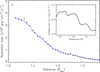 |
Fig. 15. Energy lost due to radiation with height along the loop length. Radiative loss function with temperature is also plotted as obtained from CHIANTI v.8 database at electron number density of 108.5 cm−3. |
In summary, we have found that the long coronal loop which we have studied is almost in hydrostatic equilibrium and is isothermal across and along the loop. We have found evidence of damping of Alfvén waves which carries sufficient energy to support the energy lost by the loop due to radiation.
Acknowledgments
GRG acknowledges support from the UK Commonwealth Scholarship Commission via a Rutherford Fellowship during his stay in University of Cambridge, UK. GDZ, and HEM acknowledge support by STFC (UK) via a consolidated grant to the solar/atomic physics group at DAMTP, University of Cambridge. Hinode is a Japanese mission developed and launched by ISAS/JAXA, with NAOJ as domestic partner and NASA and STFC (UK) as international partners. It is operated by these agencies in co-operation with ESA and NSC (Norway). CHIANTI is a collaborative project involving the University of Cambridge (UK), George Mason University, and the University of Michigan (USA).
References
- Aschwanden, M. J., Newmark, J. S., Delaboudinière, J., et al. 1999, ApJ, 515, 842 [NASA ADS] [CrossRef] [Google Scholar]
- Aschwanden, M. J., Nitta, N. V., Wuelser, J.-P., & Lemen, J. R. 2008, ApJ, 680, 1477 [NASA ADS] [CrossRef] [Google Scholar]
- Asgari-Targhi, M., van Ballegooijen, A. A., & Imada, S. 2014, ApJ, 786, 28 [NASA ADS] [CrossRef] [Google Scholar]
- Banerjee, D., Teriaca, L., Doyle, J. G., & Wilhelm, K. 1998, A&A, 339, 208 [NASA ADS] [Google Scholar]
- Banerjee, D., Pérez-Suárez, D., & Doyle, J. G. 2009, A&A, 501, L15 [NASA ADS] [CrossRef] [EDP Sciences] [Google Scholar]
- Bemporad, A., & Abbo, L. 2012, ApJ, 751, 110 [NASA ADS] [CrossRef] [Google Scholar]
- Brooks, D. H., & Warren, H. P. 2016, ApJ, 820, 63 [NASA ADS] [CrossRef] [Google Scholar]
- Cranmer, S. R., van Ballegooijen, A. A., & Edgar, R. J. 2007, ApJS, 171, 520 [Google Scholar]
- Cranmer, S. R., & Winebarger, A. R. 2019, ARA&A, in press [arXiv:1811.00461] [Google Scholar]
- Culhane, J. L., Harra, L. K., James, A. M., et al. 2007, Sol. Phys., 243, 19 [Google Scholar]
- De Moortel, I., & Nakariakov, V. M. 2012, R. Soc. London Philos. Trans. Ser. A, 370, 3193 [Google Scholar]
- Del Zanna, G. 2013, A&A, 555, A47 [NASA ADS] [CrossRef] [EDP Sciences] [Google Scholar]
- Del Zanna, G., & Mason, H. E. 2003, A&A, 406, 1089 [NASA ADS] [CrossRef] [EDP Sciences] [Google Scholar]
- Del Zanna, G., & Mason, H. E. 2018, Sol. Phys., 15, 5 [Google Scholar]
- Del Zanna, G., Landini, M., & Mason, H. E. 2002, A&A, 385, 968 [NASA ADS] [CrossRef] [EDP Sciences] [Google Scholar]
- Del Zanna, G., Andretta, V., Poletto, G., et al. 2009, in The Second Hinode Science Meeting: Beyond Discovery-Toward Understanding, eds. B. Lites, M. Cheung, T. Magara, J. Mariska, & K. Reeves, ASP Conf. Ser., 415, 315 [NASA ADS] [Google Scholar]
- Del Zanna, G., Dere, K. P., Young, P. R., Landi, E., & Mason, H. E. 2015, A&A, 582, A56 [NASA ADS] [CrossRef] [EDP Sciences] [Google Scholar]
- Del Zanna, G., Raymond, J., Andretta, V., Telloni, D., & Golub, L. 2018a, ApJ, 865, 132 [Google Scholar]
- Del Zanna, G., Gupta, G. R., & Mason, H. E. 2018b, A&A, submitted [arXiv:1905.09783] [Google Scholar]
- Dere, K. P., Landi, E., Mason, H. E., Monsignori Fossi, B. C., & Young, P. R. 1997, A&AS, 125, 149 [NASA ADS] [CrossRef] [EDP Sciences] [Google Scholar]
- Doschek, G. A. 2012, ApJ, 754, 153 [NASA ADS] [CrossRef] [Google Scholar]
- Doschek, G. A., Mariska, J. T., Warren, H. P., et al. 2007, ApJ, 667, L109 [NASA ADS] [CrossRef] [Google Scholar]
- Doyle, J. G., Banerjee, D., & Perez, M. E. 1998, Sol. Phys., 181, 91 [NASA ADS] [CrossRef] [Google Scholar]
- Ghosh, A., Tripathi, D., Gupta, G. R., et al. 2017, ApJ, 835, 244 [NASA ADS] [CrossRef] [Google Scholar]
- Gupta, G. R. 2017, ApJ, 836, 4 [NASA ADS] [CrossRef] [Google Scholar]
- Gupta, G. R., Tripathi, D., & Mason, H. E. 2015, ApJ, 800, 140 [NASA ADS] [CrossRef] [Google Scholar]
- Hahn, M., & Savin, D. W. 2013, ApJ, 776, 78 [NASA ADS] [CrossRef] [Google Scholar]
- Hahn, M., & Savin, D. W. 2014, ApJ, 795, 111 [NASA ADS] [CrossRef] [Google Scholar]
- Hahn, M., Landi, E., & Savin, D. W. 2012, ApJ, 753, 36 [NASA ADS] [CrossRef] [Google Scholar]
- Hara, H., Watanabe, T., Harra, L. K., Culhane, J. L., & Young, P. R. 2011, ApJ, 741, 107 [NASA ADS] [CrossRef] [Google Scholar]
- Hassler, D. M., Rottman, G. J., Shoub, E. C., & Holzer, T. E. 1990, ApJ, 348, L77 [NASA ADS] [CrossRef] [Google Scholar]
- Klimchuk, J. A. 2009, in The Second Hinode Science Meeting: Beyond Discovery-Toward Understanding, eds. B. Lites, M. Cheung, T. Magara, J. Mariska, & K. Reeves, ASP Conf. Ser., 415, 221 [NASA ADS] [Google Scholar]
- Klimchuk, J. A., Patsourakos, S., & Cargill, P. J. 2008, ApJ, 682, 1351 [Google Scholar]
- Kosugi, T., Matsuzaki, K., Sakao, T., et al. 2007, Sol. Phys., 243, 3 [NASA ADS] [CrossRef] [Google Scholar]
- Landi, E., & Landini, M. 2004, ApJ, 608, 1133 [NASA ADS] [CrossRef] [Google Scholar]
- Lee, K.-S., Imada, S., Moon, Y.-J., & Lee, J.-Y. 2014, ApJ, 780, 177 [NASA ADS] [CrossRef] [Google Scholar]
- Lin, H., Penn, M. J., & Tomczyk, S. 2000, ApJ, 541, L83 [NASA ADS] [CrossRef] [Google Scholar]
- Markwardt, C. B. 2009, in Astronomical Data Analysis Software and Systems XVIII, eds. D. A. Bohlender, D. Durand, & P. Dowler, ASP Conf. Ser., 411, 251 [NASA ADS] [Google Scholar]
- Mathioudakis, M., Jess, D. B., & Erdélyi, R. 2013, Space Sci. Rev., 175, 1 [NASA ADS] [CrossRef] [Google Scholar]
- Moran, T. G. 2001, A&A, 374, L9 [NASA ADS] [CrossRef] [EDP Sciences] [Google Scholar]
- Oran, R., Landi, E., van der Holst, B., Sokolov, I. V., & Gombosi, T. I. 2017, ApJ, 845, 98 [NASA ADS] [CrossRef] [Google Scholar]
- Patsourakos, S., & Klimchuk, J. A. 2006, ApJ, 647, 1452 [NASA ADS] [CrossRef] [Google Scholar]
- Priest, E. R., Foley, C. R., Heyvaerts, J., et al. 1998, Nature, 393, 545 [NASA ADS] [CrossRef] [Google Scholar]
- Schmelz, J. T., Reames, D. V., von Steiger, R., & Basu, S. 2012, ApJ, 755, 33 [NASA ADS] [CrossRef] [Google Scholar]
- Testa, P., De Pontieu, B., & Hansteen, V. 2016, ApJ, 827, 99 [CrossRef] [Google Scholar]
- Tripathi, D., Mason, H. E., Dwivedi, B. N., del Zanna, G., & Young, P. R. 2009, ApJ, 694, 1256 [NASA ADS] [CrossRef] [Google Scholar]
- Ugarte, I. 2010, EIS Software Note No. 12, https://sohoftp.nascom.nasa.gov/solarsoft/hinode/eis/doc/eis_notes/12_STRAY_LIGHT/eis_swnote_12.pdf [Google Scholar]
- Van Ballegooijen, A. A., Asgari-Targhi, M., Cranmer, S. R., & DeLuca, E. E. 2011, ApJ, 736, 3 [NASA ADS] [CrossRef] [Google Scholar]
- van Ballegooijen, A. A., Asgari-Targhi, M., & Voss, A. 2017, ApJ, 849, 46 [Google Scholar]
- Watko, J. A., & Klimchuk, J. A. 2000, Sol. Phys., 193, 77 [NASA ADS] [CrossRef] [Google Scholar]
- Wilhelm, K., Fludra, A., Teriaca, L., et al. 2005, A&A, 435, 733 [NASA ADS] [CrossRef] [EDP Sciences] [Google Scholar]
- Winebarger, A. R., Warren, H. P., & Mariska, J. T. 2003, ApJ, 587, 439 [NASA ADS] [CrossRef] [Google Scholar]
- Withbroe, G. L., & Noyes, R. W. 1977, ARA&A, 15, 363 [NASA ADS] [CrossRef] [Google Scholar]
- Xie, H., Madjarska, M. S., Li, B., et al. 2017, ApJ, 842, 38 [NASA ADS] [CrossRef] [EDP Sciences] [Google Scholar]
- Young, P. 2011, EIS Software Note No. 7, https://sohoftp.nascom.nasa.gov/solarsoft/hinode/eis/doc/eis_notes/07_LINE_WIDTH/eis_swnote_07.pdf [Google Scholar]
- Young, P. 2015, EIS Software Note No. 16, https://sohoftp.nascom.nasa.gov/solarsoft/hinode/eis/doc/eis_notes/16_AUTO_FIT/eis_swnote_16.pdf [Google Scholar]
All Figures
|
Fig. 1. Intensity maps obtained from Fe X 184.54, Fe XI 188.23, Fe XII 195, and Si X 258 Å showing clear long loops in all the panels. |
| In the text | |
|
Fig. 2. Intensity maps obtained from the STEREO-B EUVI 195 Å passband showing clear long loops at different times as labelled. |
| In the text | |
|
Fig. 3. Intensity maps obtained from Fe XII 195 Å showing the loop traced out to study in detail. The quiet Sun region is also traced out for the purpose of determining the background. The white curved box indicates region chosen along the curved loop. |
| In the text | |
|
Fig. 4. Length (top panel) and width (bottom panel) of the long coronal loop with distance as obtained from the Fe XII 193 Å intensity map. |
| In the text | |
|
Fig. 5. Intensity obtained from Fe X 184.54, Fe XII 186.88*, Fe XI 188.23, Fe XII 195.12, and Si X 258.37*, 261.04 Å spectral lines along the coronal loop (left panel) and quiet Sun region (right panel) with height. The intensities are recalibrated using the method of Del Zanna (2013). The asterisks denote respective spectral lines are density sensitive. Horizontal lines denote expected level of scattered light as per Ugarte (2010). |
| In the text | |
|
Fig. 6. Measured intensity ratios of Fe XII 193.51 and 195.12 Å lines along the coronal loop. This ratio is expected to be constant at 0.67 as per CHIANTI v.8 database (dashed line). |
| In the text | |
|
Fig. 7. Electron density obtained from the Fe XII line ratio method with (dashed lines) and without (solid lines) BS, as labelled. |
| In the text | |
|
Fig. 8. Emission measure (EM) loci curves obtained from Fe X 184.54, Fe XI 188.23, Fe XII 193.51, and Si X 261.04 Å spectral lines at different heights as labelled. |
| In the text | |
|
Fig. 9. Temperature obtained along the coronal loop as obtained from the EM-loci curves. |
| In the text | |
|
Fig. 10. Electron densities obtained from the line pair of Fe XII λ186.88/λ195.12 with and without BS plotted in right and left panels, respectively. Densities are fitted with an exponential function to obtain the density scale height which are also printed on the figures. |
| In the text | |
|
Fig. 11. Plasma filling factor obtained along the coronal loop. |
| In the text | |
|
Fig. 12. Effective velocity (combined thermal and non-thermal velocity) obtained along the coronal loop from various spectral lines as labelled. |
| In the text | |
|
Fig. 13. Non-thermal velocity obtained along the coronal loop from various spectral lines as labelled. |
| In the text | |
|
Fig. 14. Proportional Alfvén wave energy ( |
| In the text | |
|
Fig. 15. Energy lost due to radiation with height along the loop length. Radiative loss function with temperature is also plotted as obtained from CHIANTI v.8 database at electron number density of 108.5 cm−3. |
| In the text | |
Current usage metrics show cumulative count of Article Views (full-text article views including HTML views, PDF and ePub downloads, according to the available data) and Abstracts Views on Vision4Press platform.
Data correspond to usage on the plateform after 2015. The current usage metrics is available 48-96 hours after online publication and is updated daily on week days.
Initial download of the metrics may take a while.