| Issue |
A&A
Volume 627, July 2019
|
|
|---|---|---|
| Article Number | A52 | |
| Number of page(s) | 9 | |
| Section | Stellar atmospheres | |
| DOI | https://doi.org/10.1051/0004-6361/201834927 | |
| Published online | 01 July 2019 | |
Magnetic activity of the young solar analog V1358 Orinis
1
Konkoly Observatory, Research Center for Astronomy and Earth Sciences, Hungarian Academy of Sciences,
Budapest,
Hungary
e-mail: kriskovics.levente@csfk.mta.hu
2
Leibniz Institute for Astrophysics (AIP),
Potsdam,
Germany
Received:
19
December
2018
Accepted:
20
May
2019
Context. Young, fast-rotating single stars can show dramatically different magnetic signatures and levels of magnetic activity as compared with the Sun. While losing angular momentum due to magnetic breaking and mass loss through stellar winds, the stars gradually spin down resulting in decreasing levels of activity. Studying magnetic activity on such solar analogues plays a key role in understanding the evolution of solar-like stars and allows a glimpse into the past of the Sun as well.
Aims. In order to widen our knowledge of the magnetic evolution of the Sun and solar-like stars, magnetic activity of the young solar analog V1358 Ori is investigated.
Methods. Fourier analysis of long-term photometric data is used to derive rotational period and activity cycle length, while spectral synthesis is applied to high-resolution spectroscopic data in order to derive precise astrophysical parameters. Doppler imaging is performed to recover surface-temperature maps for two subsequent intervals. Cross-correlation of the consecutive Doppler maps is used to derive surface differential rotation. The rotational modulation of the chromospheric activity indicators is also investigated.
Results. An activity cycle of ~1600 days is detected for V1358 Ori. Doppler imaging revealed a surface-temperature distribution dominated by a large polar cap with a few weaker features around the equator. This spot configuration is similar to other maps of young solar analogs from the literature, and supports recent model predictions. We detected solar-like surface differential rotation with a surface shear parameter of α = 0.016 ± 0.010, which is in close agreement with our recently proposed empirical relation between rotation and differential rotation. The chromospheric activity indicators showed rotational modulation.
Key words: stars: activity / stars: imaging / starspots / stars: individual: V1358 Ori
© ESO 2019
1 Introduction
Studying magnetic activity, which is one of the indicators of the state of the underlying magnetic dynamo, is important for our understanding of the evolution of solar-like stars along the main sequence, since the magnetic dynamo strongly affects not just the stellar structure (Berdyugina 2005), but also the spin-down of the star due to magnetic breaking (e.g., Barnes 2003), angular momentum loss through stellar winds (MacGregor & Brenner 1991), and so on.
Strong magnetic activity could also affect orbiting planetary systems through strong stellar winds or high-energy electromagnetic or particle radiation, which may ultimately erode planetary atmospheres as well (e.g., Vida et al. 2017).
Solar magnetic fields are generated by an αΩ-type dynamo (Parker 1955). Here, the poloidal field is wound up and amplified by the differential rotation creating the toroidal field (Ω effect), while the α effect creates small-scale poloidal fields from the toroidal field via rotationally induced convective turbulence, and turbulent diffusion builds up the large-scale poloidal field by reconnection of the small-scale field.
In rapidly rotating late-type (G–K) dwarfs, the Ω-effect can be suppressed, resulting in an α2Ω type dynamo (see Ossendrijver 2003, and references therein, or e.g., Kővári et al. 2004 for observational evidence). However, as these stars evolve,they spin down mostly due to magnetic breaking (Skumanich 1972, Barnes 2003), hence their dynamo shift from the α2 Ω domain to the αΩ (Ossendrijver 2003).
In orderto properly understand the magnetic evolution of the Sun and solar-like stars along the main sequence (and its effect on their vicinity), it is imperative to study the magnetic activity of young solar-type stars.
V1358 Ori (HD 43989, HIP 30030) was originally identified as an active star and potential Doppler imaging target and classified as G0IV by Strassmeier et al. (2000). Later it was reclassified as an F9 dwarf by Montes et al. (2001), which was confirmed by McDonald et al. (2012). Vican & Schneider (2014) estimated the effective temperature to be Teff = 6100 K. They also reported infrared excess based on WISE data and suggested the presence of a debris disk around the star. Zuckerman et al. (2011) identifies V1358 Ori as a member of the Columba association, and thus a very young (≈ 30 Myr) solar analog.
Hackman et al. (2016) carried out a Zeeman–Doppler analysis of V1358 Ori. These latter authors reported a strong toroidal magnetic field component on the Stokes V maps, and prominent polar features on the brightness map, as well as some weaker, lower-latitude spots; however their phase-coverage was poor.
In this paper, we carry out a photometric and spectroscopic analysis of the young solar analog V1358 Ori, based on an 18-yr homogeneous photometric data set and Doppler imaging applied to high-resolution spectra covering two rotations. We also derive surface differential rotation from the consecutive Doppler maps and compare the results to similar young active solar analogs.
2 Observations
Strömgren (by) photometric data and Johnson-Cousins V IC data were gathered with Wolgang and Amadeus, the 0.75 m automatic photoelectric telescopes operated by the Leibniz Institute for Astrophysics Potsdam, and located at Fairborn Observatory, Arizona (Strassmeier et al. 1997) between 4 March 1997 and 8 March 2015. All differential measurements were taken with respect to the comparison star HD 44517. Between 4 March 1997 and 16 April 1997, the check star was HD 44019. After that, HD 45215 was used. For details on the data reduction, see Strassmeier et al. (1997) and Granzer et al. (2001). Photometric V y data are plotted in Fig. 1. We note that there is a 0.025 mag shift between the Stromgren y data of the first two seasons and the rest of the observations, which is probably due to the different transmission characteristics of the two passbands.
Spectroscopic observations were gathered via OPTICON with the NARVAL high-resolution echelle spectropolarimeter mounted on the 2 m Bernard Lyot Telescope of Observatoire Midi-Pyrénées at Pic du Midi, France, between 9 and 20 December 2013 (see Table 1). A peak resolution of R = 80 000 was reached in spectroscopic object mode. The exposure time was texp = 1200 s, yielding a typical signal-to-noise ratio (S/N) of ≈300.
To phase the observations, the following ephemeris was used:
 (1)
(1)
T0 was adoptedfrom Hackman et al. (2016). For details on the rotational period, see Sect. 3.
Spectroscopic data reduction was carried out with the standard NARVAL data-reduction pipeline. ThAr arc-lamps were used for wavelength calibration. An additional continuum fit and normalization were applied in order to avoid erroneous continuum fits during the spectral synthesis and Doppler inversion.
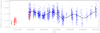 |
Fig. 1 Strömgren y (red) and Johnson V (blue) differential photometry of V1358 Ori. The overplotted curve is the combination of the two long-term cycles. See text for details. |
Spectroscopic observing log for V1358 Ori.
3 Photometric analysis
The period analyses were carried out on the Johnson V data. Strömgren y data were excluded as they only consist of 458 points and there is a long gap at the beginning of the time series (see Fig. 1).
For photometric period determination, we used MuFrAn1, a code for frequency analysis based on Fourier transformation (Kolláth 1990; Csubry & Kolláth 2004). We accepted the peak at the cycle-per-day value of c∕d = 0.7368 yielding Prot = 1.3571 d as the rotational period, which is close to the period derived by Cutispoto et al. (2003, Prot = 1.16 d). The reasoning behind this is the following. We gradually pre-whitened the Fourier spectra with the two peaks corresponding to the two long-term changes (≈1600 and ≈5200 days; see Fig. 2), the suspected rotational period, and the “forest” of peaks around that value, and a signal of one day caused by the binning of the data (two or three consecutive measurements were taken in V and I each day). The resulting Fourier spectrum contained no signal which could reasonably be considered to be real within the precision of the photometry. Since the only period is that of 1.3571 d which cannot be attributed to an artificial origin or a long-term cyclic behavior, we accepted it as the rotational period. Moreover, only Prot = 1.3571 d yields a properly phased light curve. The result is very close to the average of the seasonal periods (Prot = 1.3618 d) and is also consistent with the measured v sin i value (see Sect. 4).
Figure 3 shows the seasonally phased V light curves to demonstrate the robustness of the derived photometric period. Solid lines indicate a two-spot analytic spot model fitted to each season using SpotModel (SML; Ribárik et al. 2003). On the plot of the fourth season, both active longitudes are weak, while in the case of the seventh season, it is hard to decide which is the dominant longitude. Seasons where the low number of points made inspection impossible were omitted from the plot: two between Helicoentric Julian Dates (HJD) = 2 454 557 and 2 455 092, one between 2 455 239 and 2 455 459, and two after 2 455 588. On subplots (4) and (5), that is, intervals 2 452 895.0–2 453 111.6 and 2 453 265.0–2 453 477.6, the active longitudes seem to shift from ≈0.1 and ≈0.6 to ≈0.3 and ≈0.8, while on subplot (10), 2 455 460.0–2 455 588.8, they appear to be in the previous positions again. This could indicate the presence of a flip-flop like phenomenon (Jetsu et al. 1994), with a time scale of ≈6 yr.
After visual inspection of the complete 14-yr V light curve, a possible long-term cyclic behavior can be seen as well, which was confirmed by the Fourier analysis, yielding Pcyc ≈ 1600 d (see the first Fourier-spectrum plot in Fig. 2). The sum of this cycle and the other long-term change from the Fourier analysis (≈ 5200 d) is overplotted on the complete V light curve in Fig. 1. There is a 0.025 mag systematic shift between the V and y data, which is probably due to the different transmission characteristics of the two bands, therefore we decided not to include the Strömgren data of the first two seasons in our long-term fit.
For further discussion on the spot configuration, suspected flip-flop, and the activity cycle, see Sect. 7.
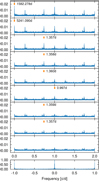 |
Fig. 2 Upper panels: Fourier spectra of the V light curve of V1358 Ori. Orange rectangles denote the strongest peaks of the subsequent steps. Consecutive plots show pre-whitened spectra with the periods shown. Bottom panel: Fourier window function. See Sect. 3 for details. |
4 Fundamental parameters
4.1 Spectroscopic analysis
Precise astrophysical parameters are fundamental for Doppler inversion, and therefore we carried out a detailed spectroscopic analysis based on spectral synthesis using the code SME (Piskunov & Valenti 2017). During the synthesis local thermodynamic equilibrium (LTE) was assumed, and MARCS models were used (Gustafsson et al. 2008). Atomic line parameters were taken from the VALD database (Kupka et al. 1999). Macroturbulence was estimated using the following equation (Valenti & Fischer 2005):
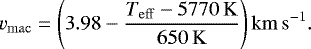 (2)
(2)
Astrophysical parameters were determined using the following methodology.
- 1.
Determination of v sin i using initial astrophysical parameters taken from Montes et al. (2001) and assuming solar abundances.
- 2.
Microturbulence (ξ) fit with same astrophysical parameters and v sin i from step 1 using lines with log gf < −2.5, since weak lines are more sensitive to the change of microturbulence.
- 3.
Refitting v sin i and ξ simultaneously to check robustness.
- 4.
Fitting Teff using solar metallicity and line broadening parameters from step 3.
- 5.
Fitting metallicity using the effective temperature value from step 4.
- 6.
Fitting log g using stronger lines (log gf > 0).
- 7.
Refitting Teff, log g, and metallicity simultaneously to check robustness.
- 8.
Refitting v sin i.
A lithium abundance fit was carried out using non-LTE departure coefficients (Piskunov & Valenti 2017). The fit yielded A(Li) = 2.27 ± 0.05. An example of the fit can be seen in Fig A.1. The astrophysical parameters are summarized in Table 2.
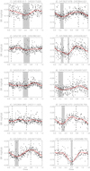 |
Fig. 3 Seasonal light curves of V1358 Ori phased with Prot = 1.3571 d. The time periods are denoted over the plots in JD along with the number of the seasons. Solid (red) lines show a two-spot model fitted to the light curves. Shaded zones show the longitudinal position of the dominant spot and the width of thezone denotes the error of the spot longitude. Vertical dashed lines indicate the longitude of the weaker spot. Certain seasons were omitted where a low number of data points made visual inspection meaningless. |
Fundamental astrophysical parameters of V1358 Ori.
4.2 Distance, radius, and inclination
The Gaia DR2 parallax of π = 19.22 ± 0.05 mas (Gaia Collaboration 2016, 2018) gives a distance of d = 52 ± 1.3 pc. This distance using the average V brightness of the star yields a bolometric magnitude of  (with extinction from Schlafly & Finkbeiner 2011 and bolometric correction from Flower 1996 taken into account). This results in a luminosity of
  , which is in good agreement with the value from Gaia DR2 (L∕L⊙ = 1.64 ± 0.015, Gaia Collaboration 2018), and thus a radius of R∕R⊙ = 1.17 ± 0.03. The radius with the photometric period and the v sin i = 38 ± 1 km s−1 from the spectral synthesis yields an inclination of i = 60 ± 10°.
4.3 Age
The lithium abundance from the spectral synthesis using the empirical correlation between age and abundance from Carlos et al. (2016) would yield t ≈ 0.75 ± 0.5 Gyr. However, it was pointed out by Balachandran (1990) and Eggenberger et al. (2010), for example, that in case of fast-rotating stars, lithium abundance is not always a suitable age indicator. Lithium depletion is also dependent on the spectral type: on an M dwarf, Li can be depleted in 10 Myrs, while on a hotter star, this rate is much lower.
According to Zuckerman et al. (2011), for example, V1358 Ori is a member of the Columba association, which has an age of ~ 30 Myr. This is in good agreement with the computed gyrochronological age (tgyro = 23 ± 7 Myr using Eq. (5.3) in Barnes 2009). Therefore, it is most likely that V1358 Ori is a very young solar analog.
5 Doppler imaging
5.1 The next-generation code iMap
Our Doppler imaging code iMap (Carroll et al. 2012) carries out multi-line Doppler inversion on a list of photospheric lines between 5000 and 6750 Å. We included 40 virtually nonblended absorption lines with suitable line depth and temperature sensitivity, and well-defined continuum. The stellar surface is divided into 5° × 5° segments. For each local line profile, the code uses a full radiative solver (Carroll et al. 2008). The local line profiles are then disk integrated and the individually modeled, disk-integrated lines are averaged. Atomic line data are taken from VALD (Kupka et al. 1999). Model atmospheres are taken from Castelli & Kurucz (2004) and are interpolated for the necessary temperature, gravity, or metallicity values. Due to the high computational capacity requirements, LTE radiative transfer is used instead of spherical model atmospheres, but imperfections in the fitted line shapes are well compensated by the multi-line approach. Additional input parameters are micro- and macroturbulence, and v sin i.
For the surface reconstruction, an iterative regularization method based on a Landweber algorithm was used (Carroll et al. 2012), meaning no additional constraints are imposed in the image domain. According to our tests (see Appendix A of Carroll et al. 2012 for details), the iterative regularization proved to be effective and inversions based on the same datasets always converged to the same image solution.
5.2 Surface reconstructions
The available 15 spectra are divided into two subsets. The corresponding time intervals are 2 456 636.43–2 456 639.66 and 2 456 641.42–2 456 647.65. The first subset consists of eight spectra and covers 2.4 rotations, while the other seven spectra of the second subset cover 4.6 rotations. The phase coverages are not completely uniform, nevertheless both subsets are suitable for Doppler imaging.
The two resulting Doppler reconstructions (henceforth S1 and S2) for V1358 Ori are plotted in Fig. 4. The average profiles are plotted along with the final profile fits (thick black and thin red lines, respectively) in Fig 5.
The overall characteristics of the two individual Doppler reconstructions are relatively similar. This is supported by the average Doppler image using all the available spectra; see Fig. 6. The resulting average map is relatively similar to the two individual images in Fig. 4, indicating only minor changes in the spot configuration.
Doppler imaging reveals a strong polar cap, as well as both cool and hot features at lower latitudes, down to the equator. Spot temperatures range from ≈4500 K to ≈ 6400 K; this latter is ≈350 K higher than the temperature of the quiet photosphere. The contrast of the coolest features of ≈ 1500 K relative to the unspotted photosphere is close to the typical value for a late F, early G dwarf (Berdyugina 2005).
The shape of the polar feature changes somewhat from S1 to S2: while on S1, the spot features an appendage reaching ≈ 45° latitude around 0.4 phase, another eccentricity is seen at ≈ 0.7 on S2. There is a fainter cool feature around 30° latitude and 0.9 phase, which almost completely disappears on S2, however the sub-equatorial spot around 0.2 phase becomes more prominent. The other cool low-latitude feature at ≈ 0.6 phase fades somewhat, and is also displaced to ≈0.55.
There are bright features present on both maps. There is a larger one at ≈ 0.4 phase whichbecomes somewhat less prominent and has a different shape on the second image. There are also other much weaker equatorial bright spots on both maps, with slightly different shapes.
Hot features are often considered to be of artificial origin, mostly caused by insufficient phase coverage, as previous tests (e.g., Lindborg et al. 2014) have pointed out. However, decreasing the phase coverage usually introduces both cool and hot features on roughly the same longitude (Fig. 3 in Lindborg et al. 2014). Also, the two Doppler maps both show similar hot features at the same positions, and are based on completely independent datasets with different phase coverages. These features can also be seen on the average map derived from all of the spectra, where the phase coverage is inherently better, roughly at the same positions. The shape of the chromosperic activity indicator curves might also support the conclusion that the bright spots are real (see Sect. 6). Thus, we conclude that it is more likely that these hot spots are indeed real features.
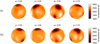 |
Fig. 4 Two consequent Doppler images of V1358 Ori plotted in four different rotational phases. The corresponding average HJDs for the maps are 2 456 638.1 and 2 456 653.9 for S1 and S2, respectively. |
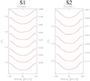 |
Fig. 5 Observed averaged line profiles and final fits for the two subsets. The dotted (black) lines represent the observations, while the solid (red) lines are the fits from the Doppler imaging. Rotational phases are marked on the right side of the plots. |
5.3 Differential rotation
Longitudinal spot displacements from the first series compared to the second can be used as a tracer of surface differential rotation. Visual inspection of the two subsequent Doppler maps may indicate such rearrangements (see Sect. 5.2): the longitudinal displacement of the subequatorial cool spot around 0.4 phase or the displacement and change of shape of the bright feature at ≈ 0.6 phase can be interpreted as such.
Surface differential rotation can be measured by longitudinally cross-correlating consecutive Doppler images (Donati & Collier Cameron 1997), and fitting the latitudinal correlation peaks by an assumed quadratic rotational law (see e.g., Kővári et al. 2012):
 (3)
(3)
where Ω(β) is the angular velocity at β latitude, Ωeq is the angular velocity of the equator, and ΔΩ = Ωeq − Ωpole gives the difference between the equatorial and polar angular velocities. With these, the dimensionless surface shear parameter α is defined as α = ΔΩ∕Ωeq.
We cross-correlate the available two Doppler images to build up a 2D cross-correlation function map shown in Fig. 7. Despite some noise it is clear from the figure that the equator rotates most rapidly and the rotation velocity decreases with increasing latitude angle, that is, the correlation pattern indicates solar-type surface differential rotation on V1358 Ori. When fitting the pattern with a solar-type differential rotation law of the quadratic form above we get Ωeq = 266.8 ± 0.3° ∕day and ΔΩ = 4.3 ± 1.0° ∕day resulting in a surface shear parameter of α = 0.016 ± 0.004. Errors are estimated from the FWHMs and amplitudes of the Gaussian fits to the latitudinal bins. However, having only two consecutive Doppler images could introduce false correlation, making the cross-correlation technique less powerful (Kővári et al. 2017). Moreover, due to projection effects, the actual impact of the strongest polar features is restricted and the low-latitude features are less contrasted. As a result, the true errors of the derived surface shear may be somewhat larger, therefore we assume error bar of ±0.01 for α instead of the formal value of ±0.004 from the fit.For further discussion on the differential rotation, see Sect. 7.
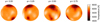 |
Fig. 6 Average Doppler image of V1358 Ori derived using all of the spectra plotted in four rotational phases. |
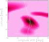 |
Fig. 7 Cross-correlation function map obtained by cross-correlating the two subsequent surface maps shown in Fig. 4. Darker regions correspond to stronger correlation. The best-fit rotation law to the correlation peaks (dots) suggests solar-type differential rotation with a surface shear of α = 0.016. |
6 Chromospheric activity
We measured the Ca II RHK, Hα, and Ca II infrared triplet (IRT) chromospheric activity indices for all of the spectra individually to see if there is any rotational modulation present for the two covered rotations.
For the RHK, we first calculated the noncalibrated S-index as described in Vaughan et al. (1978). The instrumental values were then transformed into the original Mt. Wilson scale with the calibration coefficients for NARVAL derived by Marsden et al. (2014). To avoid color-dependence, S-index values were transformed to RHK (Middelkoop 1982; Rutten 1984). To subtract the photospheric adjunct, we applied the correction formula of Noyes (1984). For the Hα, we used the indicator defined by Kürster et al. (2003). The IRT index was calculated using the formula of Marsden et al. (2014).
The apparent average surface-temperatures were also computed for the two Doppler images in the same phases for comparison. The RHK, Hα, and the IRT indices are plotted in Fig. 8 along with average temperatures. The values themselves are summarized in Table 3. The errors were estimated using error propagation and are on the order of 0.004, 0.003, and 0.001 for RHK, Hα, and IRT, respectively.
All of the indices clearly show some change with the rotational phases which could be interpreted as rotational modulation. Apart from a few outlying points, the RHK, Hα, and IRT indices show roughly the same behavior. The overall shape of the curves is similar, but there is no clear correlation between the position of the maximal chromospheric activity and the highest spot coverage (i.e., the lowest average surface-temperature). One might argue that the largest difference between the chromospheric activity and the average surface-temperature is around 0.2–0.4 phase, where, on the Doppler images, the strongest hot spot becomes gradually visible, which might indicate that the hot structure has a chromospheric counterpart (and further strengthen the hypothesis that these features are indeed not artifacts of the Doppler imaging process).
7 Discussion
Both visual inspection and the Fourier analysis suggest a possible activity cycle of ≈ 1600 d, that is, ≈ 4.5 yr. The additional Strömgren y photometry (see Fig. 1) also seems to confirm this cycle, but these data were not included in the Fourier analysis, as the Strömgren y filter is much narrower than the Johnson V (23 vs. 88 nm) and there is also a large gap in those observations. The rotational period and the length of the activity cycle are two important observables of magnetically active stars. Their ratio is related to the dynamo number which is an indicator of magnetic activity. The derived rotational period and the long-term cycles (including the suspected one of ≈ 5200 days) both show a close fit to the rotational period–activity cycle length relation derived by Oláh et al. (2016) (see Fig. 5 and details therein).
In subplot (3), HJD = 2 452 533 − 2 452 473, (4), 2 452 894–2 453 111, and (8), 2 454 370–2 454 557 of Fig. 3, the amplitudes of the light curves are significantly lower than in the other seasons. This may be a prelude to the actual flip-flop phenomenon: the stronger active region gradually weakens, while the weaker one becomes stronger.
The suspected flip-flop period of ~ 6 yr would fit the flip-flop periods found on single dwarfs by Elstner & Korhonen (2005). These latter authors pointed out that the presence of the flip-flop mechanism shows little to no dependence on the thickness of the convective layer (and hence the spectral type), however they suspected a stronger dependence on the strength of the surface differential rotation. These authors also found that the reported flip-flop periods of several years (≈ 4−9) are found in the range of |α| = |ΔΩ∕Ωeq|≈ 0.015 − 0.15 (see Elstner & Korhonen 2005 and references therein). Our values (α = 0.016 ± 0.01 and Pff ≈ 6 yr) fit this suspected relation well.
We note, however, that between the last two plotted seasons, a season was omitted due to the low number of points, therefore the above period is an upper estimate.
The surface of V1358 Ori is dominated by a large polar structure of high contrast accompanied by a low number of low-latitude, weaker features. While polar features are not uncommon on active stars in general, this configuration seems to be a recurring phenomenon on young, single solar analogs. Järvinen et al. (2008) reported a very similar and rather stable surface structure onthe young G2V star V889 Her using Doppler imaging, and later Kővári et al. (2011) derived a similar surface structure. Marsden et al. (2005) also detected a dominant polar cap without any significant low-latitude features on V557 Car, a roughly 40 Myr-old G2 solar analog. EK Dra, another young G2V star, was also reported to exhibit these features (although here with some stronger low-latitude spots as well) by Järvinen et al. (2007). Hackman et al. (2016) also derived strong polar structures and weaker equatorial features (and magnetic field configurations consistent with this picture) for V1358 Ori and another two young solar-like stars, AH Lep and HD 29615 (G3V and G2V, respectively), using Zeeman–Doppler imaging. It should be noted however that on the maps of Hackman et al. (2016), there were no bright features at all around the equator, which may indicate that the magnetic configuration has undergone structural changes. Recently, Işık et al. (2018) used numerical simulations of magnetic flux transport and emergence to model the difference in latitudinal spot distribution between the Sun and other stars. They found that as the rotation rate increases, magnetic flux emerges at higher latitudes, and a quiet region opens around the equator. They also pointed out that at eight times the rotational rate of the Sun (Prot ≈ 3 d) polar regions can form, while the width of the inactive region around the equator increases. Our findings are also consistent with this model.
Finally, we emphasize that our result of differential rotation is in agreement with the observation that active young solar-type stars exhibit weak solar-type differential rotation; for example, LQ Hya α = 0.0056 with Prot = 1.597 d, Kővári et al. 2004, or AB Dor α ≈ 0.006 with Prot = 0.5148 d, Jeffers et al. 2007. Moreover, Kővári et al. (2011) derived α = 0.009 for V889 Her, with a rotational period of 1.337 days and Marsden et al. (2005) reported a surface shear of 0.012 on V557 Car (Prot = 0.557 d). Our result is also in good agreement with the empirical relation between the rotational period and the surface shear parameter of
 (4)
(4)
for single stars suggested by Kővári et al. (2017), see Fig. A.2.
The rotational modulation of the chromospheric activity indicators suggests that the positions of the chromospheric structures (plages?) more or less coincide with the positions of the photospheric nests. The most apparent difference in the shape of the curves is in the region of 0.2–0.4 phase, which coincides with the phase where the most prominent hot feature on the Doppler images of both rotations becomes visible due to the rotation of the star. This may mean that the photospheric hot features extend to the chromosphere as well, and contribute to the overall chromospheric emission.
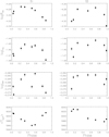 |
Fig. 8 Calcium RHK (top panels), Hα (second row), and Ca II IRT (third row) curves for the two rotations compared to the average projected surface-temperatures for the same rotational phases from Doppler imaging (bottom panels). |
Chromospheric activity indices of V1358 Ori in the observed rotational phases.
8 Summary
We carried out detailed photometric and spectroscopic analysis of the young solar analog V1358 Ori.
-
Based ona 14-yr photometric dataset we derive a rotational period of Prot = 1.3571 d for V1358 Ori.
-
An activity cycle with a period of roughly 1600 days is detected, which is consistent with the findings of Oláh et al. (2016). A flip-flop time-scale of 6 yr may also be present.
-
Using a spectral synthesis technique we determine precise astrophysical parameters for V1358 Ori.
-
We perform Doppler imaging to map the surface-temperature distribution for two subsequent epochs separated by two weeks. The surface structure is dominated by a large polar cap accompanied with weaker features at low latitudes, consistent with previous observations of young solar analogs and recent dynamo models as well. Hot features are also present on both maps.
-
Surface differential rotational is derived by cross-correlating the two subsequent Doppler images. The resulting surface shear parameter α = 0.016 ± 0.01 is in agreement with the rotational period-surface shear empirical relationship proposed recently by Kővári et al. (2017).
-
Chromospheric activity indicators are calculated and compared to the average apparent surface-temperatures. Rotational modulation is present on the activity indicator curves in both rotations. The shapes of the curves are similar. The most prominent difference between the activity indicator curves and the average surface-temperatures may indicate that the hot spots contribute to the chromospheric emission.
Acknowledgements
The authors acknowledge the Hungarian National Research, Development and Innovation Office grant OTKA K-113117, and supports through the Lendület-2012 Program (LP2012-31) of the Hungarian Academy of Sciences, and the ESA PECS Contract No. 4000110889/14/NL/NDe. K.V. is supported by the Bolyai János Research Scholarship of the Hungarian Academy of Sciences. The authors thank A. Moór for the useful conversations on stellar ages. Finally, the authors would like to thank the anonymous referee for their valuable insight.
Appendix A Additional figures
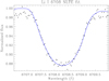 |
Fig. A.1 Example of an NLTE Li I 6708 fit. The corresponding lithium abundance is ANLTE (Li) = 2.17 ± 0.03. |
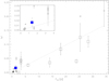 |
Fig. A.2 Absolute value of the dimensionless surface shear parameter of single stars plotted against their rotational period in days (see Kővári et al. 2017 and references therein). Circles denote results from the sheared image method, while squares indicate values obtained with the cross-correlation technique. The blue filled square indicates V1358 Ori. The dotted line represents a linear fit with a steepness of ≈ 0.005. See Sect. 7 for further details. |
References
- Balachandran, S. 1990, ApJ, 354, 310 [NASA ADS] [CrossRef] [Google Scholar]
- Barnes, S. A. 2003, ApJ, 586, 464 [NASA ADS] [CrossRef] [Google Scholar]
- Barnes, S. A. 2009, in The Ages of Stars, eds. E. E. Mamajek, D. R. Soderblom, & R. F. G. Wyse, IAU Symp., 258, 345 [NASA ADS] [Google Scholar]
- Berdyugina, S. V. 2005, Liv. Rev. Sol. Phys., 2, 8 [Google Scholar]
- Carlos, M., Nissen, P. E., & Meléndez, J. 2016, A&A, 587, A100 [NASA ADS] [CrossRef] [EDP Sciences] [Google Scholar]
- Carroll, T. A., Kopf, M., & Strassmeier, K. G. 2008, A&A, 488, 781 [NASA ADS] [CrossRef] [EDP Sciences] [Google Scholar]
- Carroll, T. A., Strassmeier, K. G., Rice, J. B., & Künstler, A. 2012, A&A, 548, A95 [NASA ADS] [CrossRef] [EDP Sciences] [Google Scholar]
- Castelli, F., & Kurucz, R. L. 2004, IAU Symp. 210, poster A20 [Google Scholar]
- Csubry, Z., & Kolláth, Z. 2004, in SOHO 14 Helio- and Asteroseismology: Towards a Golden Future, ed. D. Danesy, ESA S. P., 559, 396 [NASA ADS] [Google Scholar]
- Cutispoto, G., Messina, S., & Rodonò, M. 2003, A&A, 400, 659 [NASA ADS] [CrossRef] [EDP Sciences] [Google Scholar]
- Donati, J.-F., & Collier Cameron, A. 1997, MNRAS, 291, 1 [NASA ADS] [CrossRef] [Google Scholar]
- Eggenberger, P., Maeder, A., & Meynet, G. 2010, A&A, 519, L2 [NASA ADS] [CrossRef] [EDP Sciences] [Google Scholar]
- Elstner, D., & Korhonen, H. 2005, Astron. Nachr., 326, 278 [NASA ADS] [CrossRef] [Google Scholar]
- Flower, P. J. 1996, ApJ, 469, 355 [NASA ADS] [CrossRef] [Google Scholar]
- Gaia Collaboration, Prusti, T., et al. 2016, A&A, 595, A1 [NASA ADS] [CrossRef] [EDP Sciences] [Google Scholar]
- Gaia Collaboration (Brown, A. G. A., et al.) 2018, A&A, 616, A1 [NASA ADS] [CrossRef] [EDP Sciences] [Google Scholar]
- Granzer, T., Weber, M., & Strassmeier, K. G. 2001, Astron. Nachr., 322, 295 [NASA ADS] [CrossRef] [Google Scholar]
- Gustafsson, B., Edvardsson, B., Eriksson, K., et al. 2008, A&A, 486, 951 [NASA ADS] [CrossRef] [EDP Sciences] [Google Scholar]
- Hackman, T., Lehtinen, J., Rosén, L., Kochukhov, O., & Käpylä, M. J. 2016, A&A, 587, A28 [NASA ADS] [CrossRef] [EDP Sciences] [Google Scholar]
- Işık, E., Solanki, S. K., Krivova, N. A., & Shapiro, A. I. 2018, A&A, 620, A177 [NASA ADS] [CrossRef] [EDP Sciences] [Google Scholar]
- Järvinen, S. P., Berdyugina, S. V., Korhonen, H., Ilyin, I., & Tuominen, I. 2007, A&A, 472, 887 [NASA ADS] [CrossRef] [EDP Sciences] [Google Scholar]
- Järvinen, S. P., Korhonen, H., Berdyugina, S. V., et al. 2008, A&A, 488, 1047 [NASA ADS] [CrossRef] [EDP Sciences] [Google Scholar]
- Jeffers, S. V., Donati, J.-F., & Collier Cameron, A. 2007, MNRAS, 375, 567 [NASA ADS] [CrossRef] [Google Scholar]
- Jetsu, L., Tuominen, I., Grankin, K. N., Mel’Nikov, S. Y., & Schevchenko, V. S. 1994, A&A, 282, L9 [NASA ADS] [Google Scholar]
- Kővári, Zs., Strassmeier, K. G., Granzer, T., et al. 2004, A&A, 417, 1047 [NASA ADS] [CrossRef] [EDP Sciences] [Google Scholar]
- Kővári, Zs., Frasca, A., Biazzo, K., et al. 2011, in Physics of Sun and Star Spots, eds. D. Prasad Choudhary, & K. G. Strassmeier, IAU Symp., 273, 121 [NASA ADS] [Google Scholar]
- Kővári, Zs., Korhonen, H., Kriskovics, L., et al. 2012, A&A, 539, A50 [NASA ADS] [CrossRef] [EDP Sciences] [Google Scholar]
- Kővári, Zs., Oláh, K., Kriskovics, L., et al. 2017, Astron. Nachr., 338, 903 [Google Scholar]
- Kolláth, Z. 1990, Konkoly Observatory Occasional Technical Notes, 1, 1 [Google Scholar]
- Kupka, F., Piskunov, N., Ryabchikova, T. A., Stempels, H. C., & Weiss, W. W. 1999, A&AS, 138, 119 [NASA ADS] [CrossRef] [EDP Sciences] [MathSciNet] [PubMed] [Google Scholar]
- Kürster, M., Endl, M., Rouesnel, F., et al. 2003, A&A, 403, 1077 [NASA ADS] [CrossRef] [EDP Sciences] [Google Scholar]
- Lindborg, M., Hackman, T., Mantere, M. J., et al. 2014, A&A, 562, A139 [NASA ADS] [CrossRef] [EDP Sciences] [Google Scholar]
- MacGregor, K. B., & Brenner, M. 1991, ApJ, 376, 204 [NASA ADS] [CrossRef] [Google Scholar]
- Marsden, S. C., Waite, I. A., Carter, B. D., & Donati, J.-F. 2005, MNRAS, 359, 711 [NASA ADS] [CrossRef] [Google Scholar]
- Marsden, S. C., Petit, P., Jeffers, S. V., et al. 2014, MNRAS, 444, 3517 [NASA ADS] [CrossRef] [Google Scholar]
- McDonald, I., Zijlstra, A. A., & Boyer, M. L. 2012, MNRAS, 427, 343 [NASA ADS] [CrossRef] [Google Scholar]
- Middelkoop, F. 1982, A&A, 107, 31 [NASA ADS] [Google Scholar]
- Montes, D., López-Santiago, J., Gálvez, M. C., et al. 2001, MNRAS, 328, 45 [NASA ADS] [CrossRef] [MathSciNet] [Google Scholar]
- Noyes, R. W. 1984, Adv. Space Res., 4, 151 [NASA ADS] [CrossRef] [Google Scholar]
- Oláh, K., Kővári, Zs., Petrovay, K., et al. 2016, A&A, 590, A133 [NASA ADS] [CrossRef] [EDP Sciences] [Google Scholar]
- Ossendrijver, M. 2003, A&ARv, 11, 287 [Google Scholar]
- Parker, E. N. 1955, ApJ, 122, 293 [NASA ADS] [CrossRef] [Google Scholar]
- Piskunov, N., & Valenti, J. A. 2017, A&A, 597, A16 [NASA ADS] [CrossRef] [EDP Sciences] [Google Scholar]
- Ribárik, G., Oláh, K., & Strassmeier, K. G. 2003, Astron. Nachr., 324, 202 [NASA ADS] [CrossRef] [Google Scholar]
- Rutten, R. G. M. 1984, A&A, 130, 353 [NASA ADS] [Google Scholar]
- Schlafly, E. F., & Finkbeiner, D. P. 2011, ApJ, 737, 103 [NASA ADS] [CrossRef] [Google Scholar]
- Skumanich, A. 1972, ApJ, 171, 565 [NASA ADS] [CrossRef] [Google Scholar]
- Strassmeier, K. G., Boyd, L. J., Epand, D. H., & Granzer, T. 1997, PASP, 109, 697 [NASA ADS] [CrossRef] [Google Scholar]
- Strassmeier, K., Washuettl, A., Granzer, T., Scheck, M., & Weber, M. 2000, A&AS, 142, 275 [NASA ADS] [CrossRef] [EDP Sciences] [Google Scholar]
- Valenti, J. A.,& Fischer, D. A. 2005, ApJS, 159, 141 [NASA ADS] [CrossRef] [MathSciNet] [Google Scholar]
- Vaughan, A. H., Preston, G. W., & Wilson, O. C. 1978, PASP, 90, 267 [NASA ADS] [CrossRef] [Google Scholar]
- Vican, L., & Schneider, A. 2014, ApJ, 780, 154 [NASA ADS] [CrossRef] [Google Scholar]
- Vida, K., Kövári, Zs., Pál, A., Oláh, K., & Kriskovics, L. 2017, ApJ, 841, 124 [NASA ADS] [CrossRef] [Google Scholar]
- Zuckerman, B., Rhee, J. H., Song, I., & Bessell, M. S. 2011, ApJ, 732, 61 [NASA ADS] [CrossRef] [Google Scholar]
All Tables
All Figures
|
Fig. 1 Strömgren y (red) and Johnson V (blue) differential photometry of V1358 Ori. The overplotted curve is the combination of the two long-term cycles. See text for details. |
| In the text | |
|
Fig. 2 Upper panels: Fourier spectra of the V light curve of V1358 Ori. Orange rectangles denote the strongest peaks of the subsequent steps. Consecutive plots show pre-whitened spectra with the periods shown. Bottom panel: Fourier window function. See Sect. 3 for details. |
| In the text | |
|
Fig. 3 Seasonal light curves of V1358 Ori phased with Prot = 1.3571 d. The time periods are denoted over the plots in JD along with the number of the seasons. Solid (red) lines show a two-spot model fitted to the light curves. Shaded zones show the longitudinal position of the dominant spot and the width of thezone denotes the error of the spot longitude. Vertical dashed lines indicate the longitude of the weaker spot. Certain seasons were omitted where a low number of data points made visual inspection meaningless. |
| In the text | |
|
Fig. 4 Two consequent Doppler images of V1358 Ori plotted in four different rotational phases. The corresponding average HJDs for the maps are 2 456 638.1 and 2 456 653.9 for S1 and S2, respectively. |
| In the text | |
|
Fig. 5 Observed averaged line profiles and final fits for the two subsets. The dotted (black) lines represent the observations, while the solid (red) lines are the fits from the Doppler imaging. Rotational phases are marked on the right side of the plots. |
| In the text | |
|
Fig. 6 Average Doppler image of V1358 Ori derived using all of the spectra plotted in four rotational phases. |
| In the text | |
|
Fig. 7 Cross-correlation function map obtained by cross-correlating the two subsequent surface maps shown in Fig. 4. Darker regions correspond to stronger correlation. The best-fit rotation law to the correlation peaks (dots) suggests solar-type differential rotation with a surface shear of α = 0.016. |
| In the text | |
|
Fig. 8 Calcium RHK (top panels), Hα (second row), and Ca II IRT (third row) curves for the two rotations compared to the average projected surface-temperatures for the same rotational phases from Doppler imaging (bottom panels). |
| In the text | |
|
Fig. A.1 Example of an NLTE Li I 6708 fit. The corresponding lithium abundance is ANLTE (Li) = 2.17 ± 0.03. |
| In the text | |
|
Fig. A.2 Absolute value of the dimensionless surface shear parameter of single stars plotted against their rotational period in days (see Kővári et al. 2017 and references therein). Circles denote results from the sheared image method, while squares indicate values obtained with the cross-correlation technique. The blue filled square indicates V1358 Ori. The dotted line represents a linear fit with a steepness of ≈ 0.005. See Sect. 7 for further details. |
| In the text | |
Current usage metrics show cumulative count of Article Views (full-text article views including HTML views, PDF and ePub downloads, according to the available data) and Abstracts Views on Vision4Press platform.
Data correspond to usage on the plateform after 2015. The current usage metrics is available 48-96 hours after online publication and is updated daily on week days.
Initial download of the metrics may take a while.