| Issue |
A&A
Volume 627, July 2019
|
|
|---|---|---|
| Article Number | A127 | |
| Number of page(s) | 12 | |
| Section | Planets and planetary systems | |
| DOI | https://doi.org/10.1051/0004-6361/201834378 | |
| Published online | 11 July 2019 | |
Connecting planet formation and astrochemistry
Refractory carbon depletion leading to super-stellar C/O in giant planetary atmospheres
Leiden Observatory, Leiden University,
2300
RA Leiden, The Netherlands
e-mail: This email address is being protected from spambots. You need JavaScript enabled to view it.
Received:
4
October
2018
Accepted:
30
January
2019
Abstract
Combining a time-dependent astrochemical model with a model of planet formation and migration, we compute the carbon-to-oxygen ratio (C/O) of a range of planetary embryos starting their formation in the inner solar system (1–3 AU). Most of the embryos result in hot Jupiters (M ≥ MJ, orbital radius <0.1 AU) while the others result in super-Earths at wider orbital radii. The volatile and ice abundance of relevant carbon and oxygen bearing molecular species are determined through a complex chemical kinetic code that includes both gas and grain surface chemistry. This is combined with a model for the abundance of the refractory dust grains to compute the total carbon and oxygen abundance in the protoplanetary disk available for incorporation into a planetary atmosphere. We include the effects of the refractory carbon depletion that has been observed in our solar system, and posit two models that would put this missing carbon back into the gas phase. This excess gaseous carbon then becomes important in determining the final planetary C/O because the gas disk now becomes more carbon rich relative to oxygen (high gaseous C/O). One model, where the carbon excess is maintained throughout the lifetime of the disk results in hot Jupiters that have super-stellar C/O. The other model deposits the excess carbon early in the disk life and allows it to advect with the bulk gas. In this model the excess carbon disappears into the host star within 0.8 Myr, returning the gas disk to its original (substellar) C/O, so the hot Jupiters all exclusively have substellar C/O. This shows that while the solids tend to be oxygen rich, hot Jupiters can have super-stellar C/O if a carbon excess can be maintained by some chemical processing of the dust grains. The atmospheric C/O of the super-Earths at larger radii are determined by the chemical interactions between the gas and ice phases of volatile species rather than the refractory carbon model. Whether the carbon and oxygen content of the atmosphere was accreted primarily by gas or solid accretion is heavily dependent on the mass of the atmosphere and where in the disk the growing planet accreted.
Key words: planets and satellites: atmospheres / planets and satellites: composition / planets and satellites: gaseous planets / protoplanetary disks / planets and satellites: formation
© ESO 2019
1 Introduction
The carbon-to-oxygen elemental ratio (C/O) in a planetary atmosphere is dictated by the chemical properties of its natal protoplanetary disk, the details of which are complicated by chemical evolution (Eistrup et al. 2016, 2018; Cridland et al. 2017b) and planet formation history (Madhusudhan et al. 2014, 2017; Thiabaud et al. 2015; Mordasini et al. 2016; Cridland et al. 2016). However, C/O is our best tracer of planet formation because the elemental budget of carbon and oxygen have been well studied in the diffuse interstellar medium (ISM) (Whittet et al. 2013; Boogert et al. 2015) and in protoplanetary disks (Pontoppidan et al. 2014). Moreover, its variation through the disk (see Öberg et al. 2011 and Eistrup et al. 2018) can give us clues to the location and timing of the atmospheric accretion of a planet (Cridland et al. 2016; Madhusudhan et al. 2017).
Through gas accretion alone, Cridland et al. (2017b) showed that planets tend to have atmospheric C/O that exactly matches the initial C/O of the gas disk inward of the water ice line. This result depends heavily on the physical details that dictate the rate of planetary migration. In particular, Cridland et al. (2017b) invoked “planet-traps” to solve the “Type-I migration problem”, where planets with mass ≤ few M⊕ migrate into the host star faster than they grow. These traps (also called convergence zones by Mordasini et al. 2011 and Horn et al. 2012) are discontinuities in the physical properties of the disk (i.e., dust opacity, turbulence strength, and heating mechanism) that produce a converging zero-point in the net torque (Masset et al. 2006; Hasegawa & Pudritz 2013; Coleman & Nelson 2014, 2016; Cridland et al. 2016).
In planet trap models the migration of the growing planet is restricted to the radial evolution of the trap, and in the case of Cridland et al. (2017b) each of the traps converge at the water ice line late in the disk life. Coincidentally each of the growing planets were brought to the water ice line before they began accreting their gas. Water freezes out at the highest temperature of any volatile, and hence near the water ice line all volatiles are in their gas phase, and the resulting C/O of the planet is unchanged relative to the C/O of the volatiles (gas and ice) that are inherited from the pre-stellar core. So the combination of converging planet traps near the water ice line and the chemistry of the gas near the ice line is what led to the ubiquitous result reported in Cridland et al. (2017b).
While important, gas accretion may not be the sole contributor to the metallicity (and C/O) of an exoplanetary atmosphere. Indeed both Thiabaud et al. (2015) and Mordasini et al. (2016) demonstrated that when icy planetesimals accrete directly into the forming atmosphere they can evaporate (as computed by Mordasini et al. 2006, 2015) and deliver their ices and refractories (i.e., solid carbon and silicates) directly into the planetary atmospheres. Assuming efficient mixing, this mechanism would enrich the atmosphere in carbon, oxygen, and the other elements that make up the planetesimal. This could also be a plausible explanation for Jupiter’s apparent carbon enrichment relative to the Sun (Atreya et al. 2016).
The chemistry of the disk gas and ice is commonly treated simply in planet formation models. The radial distribution of the carbon and oxygen content of the gas and ice have previously been prescribed by a constant step-function (as in Öberg et al. 2011). Each outward step is located at the ice line of the most common volatiles and is caused by volatile freeze out, transferring carbon and/or oxygen from the gas to the ice phase. In this way, the position of the gas accretion of a planet relative to the ice lines in the disk midplane dictates its C/O.
An extra level of complexity can be added by considering the radial evolution of the gas and dust. In principle any radial feature in the chemistry of the gas advects inward with the bulk gas (Thiabaud et al. 2015). However the dust also radially drifts inward faster than the gas (Weidenschilling 1977), which transports volatile species across their ice line (Booth et al. 2017; Bosman et al. 2018) leading either to an enhancement or maintenance of the gaseous C/O against inward advection. In this work, we focus mostly on the effect of chemical evolution on the resulting C/O of planetary atmospheres and ignore the effect of radial evolution on the abundance of the carbon and oxygen that is incorporated in volatile species (either gas or ice).
For the carbon and oxygen coming from refractory species (solid carbon and silicates, incorporated into planetesimals), we generally assume that they stay chemically inert. The exception to this is our model of refractory carbon depletion that is based on observations of the carbon content in rocky bodies in our own solar system (Allègre et al. 2001; Lee et al. 2010; Bergin et al. 2015). Both asteroids in the main belt and our Earth show signs of carbon depletion by between 2 and 3 orders of magnitude, respectively, relative to the interstellar medium. As such Mordasini et al. (2016) included a simple model for carbon depleted refractories in their planet formation model that contributed to their findings that planetary atmospheres tend to have substellar C/O. In this work we similarly include refractory carbon depletion in the solids, however we additionally put this missing carbon back into the gas phase, allowing it to be accreted into a planetary atmosphere.
It is a common practice to compare observed chemical abundances in (exo)planetary systems to the photosphere of their host star, as it is assumed that the stellar photosphere acts as a time capsule for the chemical composition of the gas and refractory material that it accretes through its protoplanetary disk. In this work, we assume that the C/O of the stellar photosphere represents all of the carbon and oxygen that was accreted by the star over the course of its formation. Such an assumption is most relevant for stars with smaller convective cells at the top of their atmosphere so that the gas is not mixed with the inner core. Comparing the observed planetary and host star C/O is thus an important observational tool for understanding the process of planet formation. A current observational survey of host star and planet C/O done by Brewer et al. (2017) has suggested that planetary C/O tend to be super-stellar.
In this work we combine planet formation models with the chemical results from simulations using a chemical kinetics code (the BADASS-code; see McElroy et al. 2013; Walsh et al. 2015, and references therein), which combines both gas and grain-surface chemistry using an extensive network of reactions, and to this we add two models for returning refractory carbon to the gas. In this way we study the important contributors to the delivery of carbon and oxygen as well as how the temporal evolution of the disk C/O is imprinted onto the chemical structure of an exoplanetary atmosphere. In Sect. 2 we outline how the carbon and oxygen is distributed in the disk, including a carbon excess coming from the refractory dust. In Sect. 3 we outline the chemical and disk model, while in Sect. 4 the planet formation model is outlined. We outline and discuss our results in Sect. 5, and conclude in Sect. 6.
2 Distribution of solar system C/O
2.1 Stellar C/O
The stellar C/O is set by the chemical properties of gas and dust that the star accretes during its formation. In this section, we outline the initial elemental ratios that are inferred from observations of star forming regions and from within our own solar system, and show how these can be interpreted in the context of planet formation.
Often, the initial chemical state of the gas disk is assumed to match the molecular abundances of dark clouds, meaning it did not undergo any chemical processing during the initial formation of the protostar-disk system; this is the so-called inheritance scenario (featured in Fogel et al. 2011; Cleeves et al. 2014; Walsh et al. 2015; Cridland et al. 2016; Eistrup et al. 2016). Another plausible scenario is that the gas and ice chemically evolve while accreting onto the disk (Visser et al. 2009, 2011; Drozdovskaya et al. 2014, 2016). A final scenario is known as reset; this is when all of the molecules are dissociated into their base elements (Visser et al. 2009; Pontoppidan et al. 2014; Eistrup et al. 2016). The distinction between any of the scenarios is not important to the discussion of C/O, after all, the number of carbon and oxygen atoms in the gas and ice does not change. Nonetheless, which scenario initializes the chemical state of the gas disk can have a drastic impact on the chemical evolution of its volatiles (Eistrup et al. 2016). In this work we follow the initial volatile elemental abundance of Eistrup et al. (2016), where C/O = 0.34, and assume thatthe volatile molecules are inherited from the pre-stellar core.
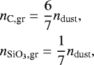
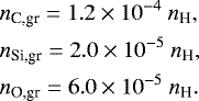
For now, we similarly assume that the initial chemical state of the refractories follows the ISM, meaning that there was no chemical interaction between the gas and refractory dust during the collapse of the cloud. If the chemical composition of the dust is representative of the ISM then it has an atomic carbon-to-silicon ratio C/SiISM = 6 (Bergin et al. 2015). Based on chemical equilibrium simulations of condensing refractories in protoplanetary disks, Alessi et al. (2017) found that the most abundant silicates have silicon-to-oxygen ratios no lower than ~ 1∕4, i.e., mostly enstatite (MgSiO3) or forsterite (MgSiO4). While they produce oxygen-bearing iron species (fayalite – Fe2 SiO4, ferrosilite – FeSiO3) within 5 AU, the majority of iron-bearing materials are troilite (FeS) and pure iron. When iron-oxides become more abundant, it is at the expense of enstatite, meaning that C/O remains unchanged, implying that refractories are generally carbon rich relative to oxygen (C/O > 1). If we assume that the dust is composed of only enstatite (Si/O = 1∕3, C/O = 2) and the Sun accretes gas and dustwith the characteristic gas-to-dust ratio (100) then we can estimate the photospheric C/O. The mean molecular weight of the gas is 2.4 g mol−1, while the molecular weight of the dust is 172.4 g mol−1 (6 carbon atoms per enstatite molecule − mmol,enstatite = 100.4 g mol−1). Hence,
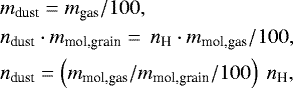
where ndust is the number of groupings of six carbon atoms and one enstatite molecule. Therefore (see a summary in Table 1),
and hence
 (1)
(1)
The volatile carbon and oxygen abundances of Eistrup et al. (2016) are nC,gas = 1.8 × 10⁻⁴ nH, and nO,gas = 5.2 × 10⁻⁴ nH. Combining these values with our computed elemental abundances from our simple refractory model, we predict a solar photosphere with C/O = 0.52, and C/Si = 15, which is close to the observed values for the Sun (0.54, ~10; Bergin et al. 2015). We can conclude two things about the solar photosphere: (1) it is carbon rich relative to the gas inherited in the protoplanetary disk, and (2) it has accreted refractories with a gas-to-dust mass ratio of at most 1001.
Carbon-to-hydrogen (C/H) and carbon-to-oxygen (C/O) ratios for the volatiles (gas), refractories (gr), and combined (tot) given the simple model (mdl) where dust mass is dominated by enstatite and solid carbon (with C/Si = 6).
2.2 Implication for planet formation
Following the above logic implies that the planets produced in Cridland et al. (2017b) have similarly substellar C/O as in Thiabaud et al. (2015) and Mordasini et al. (2016), but for different reasons. In Thiabaud et al. (2015) and Mordasini et al. (2016) the total disk (refractories and volatiles) C/O is set to solar and the carbon/oxygen component of the planet atmosphere is predominately set by the accretion of icy planetesimals directly into the (otherwise pure H/He) atmosphere. Because ice tends to be oxygen-rich, these authors predict substellar C/O. In Cridland et al. (2017b), the initial disk volatile C/O (=0.288) is dictated by the inheritance of gas from a dark cloud chemical simulation, which has substellar C/O. Since the delivery of carbon and oxygen is dominated by gas accretion in that model, their planets similarly have substellar C/O.
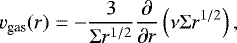
Whether a planet inherits its carbon and oxygen inventory from the gas or icy planetesimals depends on the treatment of the radial evolution of the gas. For example, Thiabaud et al. (2015) evolve the radial distribution of oxygen and carbon bearing volatiles through the disk at the radial speed of the gas,
 (2)
(2)
where Σ is the surface density of the gas and ν is the strength of viscosity.
By ignoring the transport of volatiles frozen onto grains, Eq. (2) implies that elements heavier than helium are cleared from the planet formation region of the disk (r ≲ 3 AU) in less than a 106 yr (Thiabaud et al. 2015). Including the transport and sublimation of frozen volatiles, Bosman et al. (2018) showed that the abundance of oxygen and carbon carrying volatiles can be maintained near their initial abundances over longer timescales (≳ 1 Myr), which would make them available for accretion onto a planetary atmosphere. We assume that carbon and oxygen bearing volatiles do not evolve radially, and hence only their chemical evolution is important to the abundance of elemental carbon and oxygen in either the gas or ice phases.
The substellar C/O results discussed above are currently at odds with the previously mentioned observational work that suggests that planetary atmospheres have either stellar or super-stellar C/O (Brewer et al. 2017).
2.3 Refractory carbon depletion
A final detail regarding the distribution of carbon in the protoplanetary disk was pointed out by Mordasini et al. (2016), and is based on past work (Allègre et al. 2001; Lee et al. 2010; Bergin et al. 2015), namely carbon depletion. While the ISM is carbon rich relative to silicon, the Earth is depleted in carbon by more than 3 orders of magnitude (Bergin et al. 2015). Similarly, some asteroids show intermediate levels of carbon depletion, leading Mordasini et al. (2016) to derive a simple radial distribution for the level of carbon depletion in the solar nebula, i.e.,
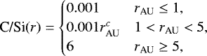 (3)
(3)
where rAU is the orbital radius in units of AU, and c ~ 5.2 is used to connect the outer (r ≥ 5 AU) and inner (r ≤ 1 AU) parts of the disk. Because of this refractory carbon depletion, solids in the Mordasini et al. (2016) model are generally more oxygen rich than assumed in this work, where the abundances are derived in Eq. (1). Such a refractory carbon depletion has been proposed to exist in other solar systems by studying the pollution of white dwarf stars, which show subsolar carbon abundances indicative of the accretion of shredded carbon-poor planetesimals (Jura 2008).
In Fig. 1 we show the graphical form of Eq. (3) in linear and log-space (inset). The source of this carbon depletion is not well constrained (see e.g. Bergin et al. 2015). Two plausible explanations involve ongoing processing of the refractory carbon through oxidation and photodissociation (Lee et al. 2010; Anderson et al. 2017), or early thermal processing of the grains as they are accreted onto the disk (Bergin et al. 2015), which is similar to the reset scenario discussed earlier. In both cases the carbon is returned to the gaseous state and would be available for accretion onto a planetary atmosphere.
The carbon that is returned to the gas quickly reacts with water to create CO. Within 1 AU, the maximum amount of carbon that is released into the gas is nearly all of the solid carbon budget inherited from the ISM. In the ISM, Mishra & Li (2015) reported Si/HISM = 40.7 ppm, which is twice as high as the value that we derive in the simple model above. When combined with C/SiISM = 6, we find an excess carbon abundance of C/Hexc = 2.44 × 10⁻⁴ (i.e., two-thirds of the total carbon) that would be released into the gas phase. This excess gaseous carbon leads to a gas disk C/O = 0.82 inside the water ice line.
Along with the increase in the refractory carbon in the disk we similarly expect a higher available refractory oxygen. To estimate this refractory component we follow Mordasini et al. (2016) who assume that the refractories have a mass ratio of 2:4:3 for thecarbon, silicates, and irons, respectively. This assumption leads to a refractory oxygen abundance of O/Href = 1.75 × 10⁻⁴.
In Fig. 2 we show two toy models for the amount of excess carbon that is available in the gas, given the two depletion mechanisms mentioned above. In the ongoing scenario oxidation or photochemistry maintains the high abundance of gaseous carbon shown in Fig. 1 over the lifetime of the gas disk. In this model, while the gas is advected into the host star rapidly (see below), inflowing dust particles from larger radii (through radial drift) are processed efficiently to maintain the carbon excess in the gas that is inferred by the carbon depletion observed today in the solids on Earth. Hence we assume that the carbon excess is maintained for the whole lifetime of the disk.
In the reset scenario we assume that all of the excess carbon is delivered early in the lifetime of the disk. This excess would then advect with the gas as it accretes onto the host star. Because there is no excess carbon advecting from larger radii, its carbon excess is not regenerated as in the ongoing scenario. We model this process by evolving the shape of the ongoing model (blue curve in Fig. 2) inward with an assumed constant advection speed vadv. The time evolving version of Eq. (3) becomes
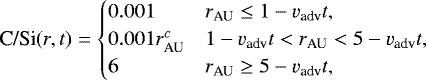 (4)
(4)
such that the excess carbon in the gas phase is

where we take vadv = 0.03 m s−1 = 6.3 AU Myr−1, which represents a typical advection speed from Bosman et al. (2018) for a gaseous disk with viscous α = 10−3. The time evolution shown in Fig. 2 is qualitatively similar to the evolution of molecular gas species shown in Thiabaud et al. (2015). As in that work, we find the radial extent of the excess carbon in the gas is lost to the host star by 0.8 Myr into the lifetime of the disk.
We note that carbon depletion does not affect the earlier prediction of the stellar photosphere, since the excess carbon that is processed off of the grains would be delivered to the gas and accrete toward the host star. Hence the number of carbon atoms accreting through the disk is preserved.
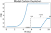 |
Fig. 1 Radial dependency of carbon depletion as described in Eq. (3). The inset shows the same plot in log-space, mimicking Fig. 2 of Mordasini et al. (2016). |
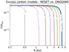 |
Fig. 2 Available excess carbon for atmospheric accretion. We assume that in the ongoing model the excess carbon is supplied by ongoing processing of dust grains, delivering the carbon to the gas. In the reset model the carbon excess is generated early in the disk life and advects with the bulk gas into the host star. |
3 Physical and chemical models of disk
For the gas and ice abundances in the disk we use the chemical results produced by Eistrup et al. (2018). A benefit in using their chemical model over that presented in Cridland et al. (2017b) is that their treatment of grain-surface chemistry is more comprehensive and includes a more extended network of chemical reactions that are relevant for determining the final abundance of carbon and oxygen-bearing molecules in both the gas and ice phases.
The most important result of Eistrup et al. (2018) is the evolution of the C/O in the gas and ice. Because of their network of surface reactions, Eistrup et al. (2018) found a departure from the typical “step function” description of C/O as first pointed out by Öberg et al. (2011). In particular, through the destructive reaction of CO in gas-grain interactions,

between the CO2 and O2 ice lines, carbon and oxygen are slowly converted from the gas phase to the ice phase (denoted by the lower case “i”). In a similar region of the disk (inward of the O2 ice line) molecular oxygen can similarly be produced on the grain surface through the reaction (Eistrup et al. 2018) as follows:

and subsequent desorption of O2.
The disk model used in Eistrup et al. (2018) was based on a power-law fit to numeric results of Alibert et al. (2013). Key features of the disk model include its cooling gas temperature and lowering surface density as the disk ages. This evolution is the main driver of the inward motion of the volatile ice lines, but also impacts the flux of ionization radiation, which depends on the surface density of the gas. The main driver of gas ionization along the disk midplane is cosmic-ray ionization whose rate depends exponentially on the gas surface density (see Eistrup et al. 2018 for details).
In Fig. 3 their evolution of C/O is presented along with the locations of the water (solid), CO2 (dashed), O2 (dotted), and CO (dot-dashed) ice lines. The step-function in C/O with steps at each of the ice lines is clearly seen, and they slowly move inward as the disk ages and cools. Outward of the CO2 ice line at times later than ~ Myr we see the conversion of gaseous CO into frozen CO2, which enhances the frozen C/O at the expense of the gaseous C/O.
This enhancement occurs between the CO2 and O2 ice lines where the most dominant molecular species in the gas (heavier than He) are CO and O2 (because of its production mentioned above), hence as CO freezes out, the gas becomes more oxygen rich (C/O decreases). The icy volatile component begins oxygen rich (primarily CO2 and H2O), and adding equal amounts of carbon and oxygen (i.e., by freezing out CO) generally increases C/O. This exchange occurs inward of the O2 ice line, where CO should tend to be gas. However, outside of the CO2 ice line when a CO molecule happens to stick to a dust grain its reaction with frozen OH proceeds faster than its desorption back to the gas phase.
This exchange of elements between the ice and gas could be important to the chemical composition of planetary atmospheres because of the relative amount of solid and gas accretion that is responsible for enhancing the atmosphere in heavier (than helium) elements.
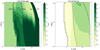 |
Fig. 3 Evolution of C/O in gas (left) and ice (right) from Eistrup et al. (2018). We note the location of the water (solid), CO2 (dashed), O2 (dotted), and CO (dot-dashed) ice lines. A step-function in C/O is seen early on in the disk’s life, which becomes complicated by chemistry as the disk ages. After ~ Myr CO is converted into frozen CO2 outward of the CO2 ice line, which lowers the gas C/O while raising the ice C/O, eventually becoming more carbon rich than the gas. |
4 Planet formation
Currently the process of planet formation through core accretion (as opposed to planet formation through gravitational instability, which is not the subject of this paper) is split into two dominant methods: planetesimal and pebble accretion. The former is discussed below and involves the accretion of large (10–100 km) bodies, while the latter describes growth through the accretion of millimeter-to-centimeter sized “pebbles” (Ormel & Klahr 2010; Lambrechts & Johansen 2014; Bitsch et al. 2015). A particular advantage of accreting pebbles over planetesimals is that the process is at least a few orders of magnitudes faster (Bitsch et al. 2015), which offers a second way of circumventing the previously mentioned Type-I migration problem.
Along with their differences in accretion rates, pebbles may also alter the delivery of heavy elements to the atmosphere of forming planets because their survivability through a proto-atmosphere is lower than that of planetesimals (Mordasini et al. 2006; Brouwers et al. 2018), and hence they should tend to deliver more refractory material to the upper atmosphere (for example, as studied by Ali-Dib 2017) than planetesimals. While this offers a possible method of differentiating the two formation mechanisms, combining pebble accretion with our chemical model is currently beyond the scope of this work.
The planet formation model used in this work is outlined in Cridland et al. (2017b) and assumes the standard planetesimal accretion paradigm. In the following section, we outline some key features of the model.
4.1 Solid accretion
In the planetesimal accretion model of planet formation (i.e., Pollack et al. 1996; Kokubo & Ida 2002; Ida & Lin 2004) planetary cores grow by first accreting from a disk of 10–100 km sized planetesimals. Known as the oligarchic phase, it has an accretion timescale of (Kokubo & Ida 2002; Ida & Lin 2004)
![Mathematical equation: \begin{align*} t_{\textrm{c,acc}} = \;& 1.2\times 10^5 \textrm{yr} \left(\frac{\Sigma_{\textrm{d}}}{10\,\textrm{g~cm}^{-2}}\right)^{-1}\left(\frac{a_{\textrm{p}}}{\textrm{AU}}\right)^{1/2}\left(\frac{M_{\textrm{c}}}{M_{\oplus}}\right)^{1/3}\nonumber\\[2pt] &\times\; \left(\frac{M_*}{M_{\odot}}\right)^{-1/6}\left[\left(\frac{\Sigma_{\textrm{g}}}{2.4\times 10^3\,\textrm{g~cm}^{-2}}\right)^{-1/5}\right.\nonumber\\[2pt] &\times\; \left. \left(\frac{a_{\textrm{p}}}{\textrm{AU}}\right)^{1/20}\left(\frac{m}{10^{18}\,\textrm{g}}\right)^{1/15}\right]^2,\end{align*}](/articles/aa/full_html/2019/07/aa34378-18/aa34378-18-eq10.png) (5)
(5)
which includes the effect of gas drag on the incoming planetesimals (terms in the square brackets). The surface density of solids (Σd) and gas (Σg) are evaluated at the radial position of the planet (ap) at each time step, and the incoming material is added to the mass of the planetary core (Mc) via Mc (t+ dt) = Mc(t)(1 + dt∕tc,acc).
Globally we assume a gas-to-dust ratio of 100, such that Σd = 0.01Σg, however as has been assumed in the past (see, e.g., Alessi et al. 2017) we enhance the amount of solid material in the planet-forming region by an order of magnitude to account for the dust trapping expected from the streaming instability (i.e., Raettig et al. 2015), which leads to the generation of planetesimals (Schäfer et al. 2017). So while the planet is undergoing oligarchic growth, Σd = 0.1Σg.
We assume that the refractory component of every planetesimal is made of the same chemical composition. The carbon and oxygen content has the same elemental abundance as derived above, i.e., C/H = 2.44 × 10⁻⁴ and O/H = 1.75 × 10⁻⁴. Meanwhile the volatile ice component follows from the results of our chemical model.
During the initial formation of the core we assume that none of the carbon and oxygen that accretes ends up in the atmosphere. This reasoning comes from work by Schlichting et al. (2015) who have shown that planetesimal accretion events are efficient at eroding atmospheres, particularly around low mass planets. This implies that any volatiles that might be out-gassed during the initial formation of the core are unlikely to survive as a proto-atmosphere. So in accounting for the elements in the atmosphere we ignore the contribution of the material that originally formed the core.
At a certain point in its evolution, the growing planet consumes or scatters most of the planetesimals in its immediate vicinity. At this point the heating from impacting planetesimals is no longer sufficient to maintain pressure support of the surrounding gas and the planet transitions from a stage of oligarchic growth to a stage of gas accretion. When this happens we assume that the original population of planetesimals is no longer present, and hence we return the gas-to-dust ratio to 100. We continue to allow planetesimal accretion during the gas accretion phase to occur (now with Σd = 0.01Σg), and it is at this point that the delivery of heavy elements to the atmosphere can begin.
As the gas envelope begins to develop we start counting the elements that are delivered into the atmosphere by solid bodies. The delivery of carbon and oxygen depends on the survival of planetesimals as they pass through the atmosphere. The thermal ablation and aerodynamic fragmentation of a planetesimal has been calculated in detail by Mordasini et al. (2015). We use a simple approach and assume that if the atmosphere is lighter than 3 M⊕ the planetesimal can fully penetrate and reach the core, while above 3 M⊕ the planetesimal is completely destroyed in the atmosphere. In the former case, only the most volatile species (e.g. CO2, H2 O) are released into the atmosphere, if they are frozen to the incoming planetesimals as computed by the chemical model; while in the latter case we assume that both the volatile ices and the refractories are distributed into the atmosphere. The critical atmosphere mass was chosen by inspecting Fig. 9 in Mordasini et al. (2015) and selecting the highest atmospheric mass where planetesimals of all sizes are destroyed in the atmosphere. This is a necessary simplification since we compute neither the internal structure of the atmosphere, nor the size distribution of the incoming planetesimals.
We note that in computing the carbon and oxygen content of the icy planetesimals we have generally ignored their radial transport that could enhance the local gas C/O (as in Booth et al. 2017) or the atmosphere directly by volatile delivery through N-body interactions after the gas disk has evaporated.
Later in its evolution, the planet opens a gap in the gas disk (see below). The gap stops the flow of dust through the disk because it forms a positive pressure gradient that traps most of the dust that is decoupled from the gas (Pinilla et al. 2016; Bitsch et al. 2018). However, the smallest grains that are still coupled to the gas dynamics can still flow across the gap (Bitsch et al. 2018), but these grains are generally about two orders of magnitude less abundant (by mass) than the typical millimeter-to-centimeter sized grains (Cridland et al. 2017a). Additionally, the gas drag that contributes to widening the effective feeding zone of the proto-planet (square brackets in Eq. (5)) vanishes. Without the gas drag, planetesimal accretion rates are reduced by about two orders of magnitude (Ida & Lin 2004). Hence, we expect the rate of solid accretion will drop when the planet opens a gap. To account for the change we reduce the surface density of solids available for accretion by two orders of magnitude (Σd= 0.0001Σg) when the gap is opened.
Finally, we set a global maximum to the amount of solid material that can be accreted by a planet. This global maximum is defined as the total solid mass in the disk, which we estimate by integrating the gas surface density profile over the whole disk (radii between 0.01 and 30 AU) and scaling it by a gas-to-dust ratio of 100.
4.2 Gas accretion
When the planet reaches a critical mass it can begin to draw down the gas from the surrounding protoplanetary disk. This process is limited by the rate of heating that the planet receives from infalling planetesimals, and the rate at which the gas can radiate away its gravitational energy. Both of these processes ultimately depend on the opacity of the envelope (κenv) (Ikoma et al. 2000; Ida & Lin 2008; Hasegawa & Pudritz 2014; Mordasini 2014; Alessi & Pudritz 2018), with the critical mass havingthe form
 (6)
(6)
and the mass accretion rate depends on the Kelvin-Helmholtz timescale
 (7)
(7)
where c and d depend on κenv (see Alessi & Pudritz 2018 for their description). Given this timescale the rate at which gas is accreted onto the planet is written as
 (8)
(8)
Given their population synthesis model, Alessi & Pudritz (2018) picked a nominal opacity of κenv = 0.001 cm2g−1 that best reproduces the population of observed exoplanets; with this opacity, c = 7.7, and d = 2.
Eventually the planet has grown to a mass of ~10 M⊕, at which point it opens a gap in the protoplanetary disk. When this happens the planet decouples from the surrounding disk and the geometry of the gas accretion changes (Szulágyi et al. 2014). In this regime the gas primarily accretes vertically onto the planet from above the midplane of the disk. Some of the gas is circulated back into the surrounding disk as described by Morbidelli et al. (2014) and illustrated by Batygin (2018).
As described by Batygin (2018), as the gas falls toward the midplane it interacts with a planetary magnetic field that dictates the dynamics of the gas within the planetary magnetosphere. Within the magnetosphere gas that falls planet-ward of the critical magnetic field line crest falls onto the planet, while gas that falls on the far side of the crest falls onto the circumplanetary disk. This gas is then recycled back into the protoplanetary disk as outlined by Morbidelli et al. (2014). Recently, Cridland (2018) derived a planetary mass accretion rate based on the following physical picture:
 (9)
(9)
where Ṁ is the gas accretion rate into the gap, RH =  is the Hill radius,
 is a scaling factor with units of length, and
  is the magnetic moment for an (assumed) magnetic dipole of magnetic field strength B and planetary radius Rp.
As argued in Cridland (2018), we set B = 500 gauss for the young planet, which assumes that the field is in equipartition with the kinetic energy of the convecting part of the planetary interior. This strength is about two orders of magnitude stronger than Jupiter’s magnetic field today, but weaker by a factor of a few than a typical brown dwarf. In effect, setting the field strength in this way represents an interpolation between our understanding of the geo- and solar dynamo (Christensen et al. 2009). For simplicity we keep the magnetic field strength constant throughout the growth of the planet, assuming that the majority of the gravitational energy of infalling gas is radiated away (i.e., a cold start model). Generally we expect the mass accretion rate to weakly depend on the magnetic field strength since Ṁ p,mag ∝ B8∕7.
As shown in Mordasini (2013), the size of the planet stays nearly constant after it has opened a gap in its disk. Hence we similarly assume that Rp does not change during this phase of planet formation. We assume that the planet has undergone a “cold-start”, such that the planet has not stored a large amount of entropy during its early stage of gas accretion (see Mordasini 2013), and Rp = 1.5 RJ.
When the gap is opened, the gas accretion is still limited by the rate at which it can release its gravitational energy, hence the true mass accretion rate is the smaller of Eqs. (8) and (9), i.e.,
 (10)
(10)
We place a similar maximum gas mass on the gas accretion as we did for the solid accretion, since our disk is on the lower mass end of known disk masses with M0 ~ 5 MJ (~ 0.005 M⊙) of gas. Hence when the planet exceeds this gas mass, it is reverted to its mass of the previous time step.
4.3 Planet migration
The planet interacts gravitationally with the gas in its protoplanetary disk, which exchanges angular momentum. The result of this interaction is that the planet changes its orbital radius, a process often called “planet migration”. The rate of migration depends on the radial structure of the gas temperature and density structure. Recently Cridland et al. (2019) outlined a method of computing the rate of planetary migration for a given disk model. The method is based on the work of Paardekooper et al. (2011) and Coleman & Nelson (2014) and includes the effect of transitions in the dust opacity and turbulent α at ice lines and the dead zone edge, respectively.
We follow the methods of Cridland et al. (2019) and compute a modified temperature profile based on a combination of the profile used in Eistrup et al. (2018), and a radially dependent dust opacity that depends on the local abundance of water and CO2 ice. Generally this warms the gas within the water ice line, because the dust opacity is higher when it is not covered with a layer of ice and flattens the temperature profile over the remainder of the disk. At the original ice line location of the Eistrup et al. (2018) disk model the gas is warmed by about 50% so that in the new disk model the ice line is shifted out by about 0.5 AU. In principle this shift changes the distribution of volatile C/O in the new disk model however such a small change does not drastically impact the chemical signature of the disk on the chemical composition of planetary atmospheres.
Changing the temperature profile has a larger effect on the total torque on the planet, which has the form (Coleman & Nelson 2014)
![Mathematical equation: \begin{align*} \Gamma_{I,\textrm{tot}} =&\, \Gamma_{\textrm{LR}} + \left[\Gamma_{\textrm{VHS}}F_{p_{\nu}}G_{p_{\nu}} + \Gamma_{\textrm{EHS}}F_{p_{\nu}}F_{p_{\chi}}\sqrt{G_{p_{\nu}}G_{p_{\chi}}} \right. \nonumber\\ &+ \left. \Gamma_{\textrm{LVCT}}\left(1-K_{p_{\nu}}\right) + \Gamma_{\textrm{LECT}}\sqrt{\left(1-K_{p_{\nu}}\right)\left(1-K_{p_{\chi}}\right)}\right],\end{align*}](/articles/aa/full_html/2019/07/aa34378-18/aa34378-18-eq20.png) (11)
(11)
where ΓLR, ΓVHS, ΓEHS, ΓLVCT, and ΓLECT are the Lindblad torques, vorticity and entropy-related horseshoe drag torques, and linear vorticity and entropy-related corotation torques, respectively (see Eqs. (3)–(7) in Paardekooper et al. 2011). The damping functions  ,
,  ,
,  ,
,  ,
,  , and
, and  are related to the ratio of either the viscous or thermal diffusion timescales with the horseshoe libration or horseshoe U-turn timescales (see Eqs. (23), (30), and (31) in Paardekooper et al. 2011). Owing to these torques the angular momentum of the planet evolves such that d L∕dt = ΓI,tot, and
 (12)
(12)
assuming the planet is a point mass in a circular, Keplerian orbit.
Each torque depends on the local gradient of the gas temperature and surface density. As an example, changes to the dust opacity can lead to a local change in the temperature gradient at the water ice line. The water ice line is the smallest radius in the disk midplane where water vapor is sufficiently cold to freeze onto dust grains. Within the ice line, the abundance of water ice smoothly changes from zero to its maximum abundance over a ~ 0.5 AU wide region. This abundance gradient leads to a smooth transition in the dust opacity because it depends on the abundance of ice frozen out on the grains (see, e.g., Miyake & Nakagawa 1993). If the water ice line inhabits a portion of the disk that is heated primarily by viscous heating, the opacity gradient in the water ice line leads to a local flattening of the gas temperature gradient. Accordingly, to maintain a constant mass accretion rate at the water ice line, the gas surface density gradient also flattens.
These changes in gradients often result in a process known as planet trapping (Lyra et al. 2010; Horn et al. 2012; Hasegawa & Pudritz 2011; Dittkrist et al. 2014), generating points of zero torque toward which planets migrate (see details outlined in Cridland et al. 2016). Generally it is assumed that trapped planets migrate with their trap until they reach their gap opening mass, which saves computing time by eliminating the need to compute the net torque on the planet (Eq. (11)). However in this work we fully compute the net torque according to Eq. (11) and the resulting change in orbital radius according to Eq. (12).
Once above the gap opening mass (Matsumura & Pudritz 2006)
 (13)
(13)
the torques responsible for the first type of planet migration (often called Type-I) disappear and the planet enters into a second phase of migration (Type-II). In this second phase planet migration proceeds on the viscous time,  , where ν = αcsH is the viscosity in the standard α-disk model (Shakura & Sunyaev 1973) and cs and H are the sound speed and scale height of the gas. With this prescription the migration rate is written as
 (14)
(14)
In the event that the planet becomes more massive than the total mass of the gas disk within its orbital radius (denoted by Mcrit) then the rate of Type-II migration is reduced by a factor of Mp /Mcrit.
In what follows, we do not invoke planet trapping, but instead compute the torques using Eqs. (11) (using the expressions from Paardekooper et al. 2011) and (12) until the gap is opened, and then we use Eq. (14).
5 Results: connecting planet formation and astrochemistry
We model the formation of 11 planets, each with different initial orbital radii equally spaced between 1 and 3 AU. For this disk model, planets starting within 1 AU tend to migrate into the host star, while planets that started at radii outside of 3 AU tend not to grow very large. All planets were initialized with masses of 0.01 M⊕ and allowed to freely migrate according to the torques computed with Eq. (11). We note that while these planets are often shown as forming in unison, in reality they are grown in isolation and no gravitational interaction between the embryos are allowed to occur.
5.1 Planet formation tracks
A convenient way of discussing the formation of a planet is through its formation track: the planet’s evolution through the mass-semimajor axis diagram as it grows. The specific details depend on the physics included in the planet formation, migration, and disk model. Hence the cases presented in this work are meant as representations of what can happen.
In Fig. 4 we show the planet formation tracks for the planets formed for this work. Planets that started with ap ≤ 2.4 AU end up as hot Jupiters, while planets starting farther out stay in the smaller super-Earth/Neptune mass range at radii between 3 and 10 AU. The outward migration of these planets is due to their interaction with a strong positive torque (see below) caused in part by the CO2 ice line, andpartly due to the properties of the outer parts of our disk model (discussed below).
The orbital properties of the planets are shown in Table 2. The general trend is that planets that start at smaller radii accrete faster, and hence do not migrate as far before their Type-II migration is slowed by their inertia. They also tend to be more massive than planets that start farther out because they accrete most of their gas in higher surface density regions of the disk.
This trend is broken for the planet that starts at 2.4 AU. For that planet we see a very slight outward migration as it interacts with the disk. This short stage of outward migration stalls its growth enough that it only accretes ~ 4 MJ of gas and ends farther out than the other hot Jupiters. Starting the planet outside of 2.4 AU places the planet in a regime of strong outward migration, moving it to lower density regions of the disk. This severely suppresses further planetary growth, resulting in the range of lower final masses. In a more in-depth study of formation history we focus on three planets, starting at 2.2 (blue), 2.4 (orange), and 2.6 (yellow) AU.
In Fig. 5 we show the individual formation tracks for the three planets along with a map of the total torque. In the map, red denotes inward migration, white is zero torque, and blue shows outward migration. The large band of outward migration that grows as the disk ages is caused by a combination of our choice of disk model (which steepens with time), and the opacity transition that occurs at the H2 O and CO2 ice lines. The mass independent outward migration feature at 10 AU is caused by a discontinuity in the temperature profile caused by our setting a minimum temperature of 20 K for radii outside of 10 AU. The color map extends up to the gap opening mass, where Type-I torques cease to be relevant for planetary migration.
In Fig. 5a we show an early snapshot of the formation tracks. Up to this point, the planets are not sufficiently massive to show significant migration, hence the tracks grow almost completely in the vertical direction.
Once the planets reach a mass of a few M⊕ they begin to feel the effect of the disk torques. In Fig. 5b the blue planet has grown so massive that it misses the band of outward migration, and begins to rapidly move inward. The orange planet has coincidentally grown to a mass where it sits in a region of zero torque, and hence has not migrated far in the first 0.5 Myr. The green planet’s growth places it in the outward migrating band, and hence it begins to migrate outward.
By Fig. 5c the blue planet has opened a gap (decoupling it from Type-I migrating torques) and its core has nearly reached its final mass. At this stage its gas accretion is limited by Eq. (9) and it is sufficiently massive that Type-II migration is also suppressed. The orange planet has grown enough to escape the region of zero torque that it has previously occupied, and begins to migrate inward rapidly. Meanwhile the green planet continues to migrate outward. Since it continues to move to larger radii, and smaller gas/solid surface densities its growth is suppressed when compared to the other planets that move inward to higher surface densities.
In Fig. 5d we show a late time in the evolution of the disk. At this point the orange planet has opened its gap and accreted nearly all of its available material. The green planet reaches the end of the outward migration band and becomes trapped between inward and outward migration. Once this planet grows enough to open a gap in the disk, it begins to move inward under Type-II migration.
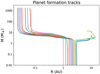 |
Fig. 4 Planet formation tracks for the synthetic planets formed in this work. There is an easily distinguishable bifurcation between the orbital evolution of the planets caused by their interaction with the disk. |
Orbital properties of the simulated planets.
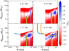 |
Fig. 5 Combined torque maps and planet formation tracks for four different snapshots throughout the formation history of our three planets of interest. In the torque maps (colored region) red denotes inward migration, white denotes zero net torque, and blue denotes outward migration. The band of outward migration between 1 and 10 AU is caused by our choice of disk model and the opacity arising from CO2 freeze out. |
5.2 Carbon-to-oxygen ratio
In Fig. 6 we have overplotted the evolving map of C/O with the orbital radius evolution for the three planets along with excess C/O that is generated by the reset scenario of refractory carbon destruction (dark green regionwithin 5 AU). In the case of the ongoing scenario, the dark green region of the figure would extend for the whole life of the disk, while in the reset scenario it eventually vanishes. In this figure, we illustrate the chemical implication of the migration history of the planets. Along the tracks we denote three important milestones with points (starting from the bottom): the point when the planet begins accreting gas, when it has accreted 3 M⊕ of gas, and when it has accreted half of its mass.
While all three of the planets begin their gas accretion at nearly the same time, their migration histories can end up delaying when they hit the later milestones. For example, the blue and orange planets both end up in a similar mass regime, but since the orange planet’s early migration was slower than the blue planet, it did not reach its half mass until ~ 1 Myr later. Similarly, since the green planet underwent significant outward migration, the point where it reached 3 M⊕ of gas was delayed by up to ~3 Myr relativeto the two other planets.
When and where planets accrete their material has important implications for the chemical make-up of their atmosphere. We note that we used a simple prescription for determining if refractories are delivered to the planetary atmosphere during a planetesimal collision. When the atmosphere is heavier than 3 M⊕ the planetesimal is completely destroyed, releasing its entire abundance of refractories and volatiles. Below this cut off, only the volatiles are delivered to the atmosphere.
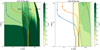 |
Fig. 6 Similar to Fig. 3, but including the effect of the excess gaseous carbon caused by the reset scenario of carbon depletion. The carbon advects inward quickly, disappearing before 1 Myr. The ongoing scenario would maintain the same level of carbon excess over the lifetime of the disk. Additionally we overplot the radial evolution of the three targeted planets. The dots along each track denote thepoint at which (starting from the bottom) the planet begins accreting gas, when it has accreted 3 M⊕ of gas, and when the planet has reached half of its final mass. The inner two planets accrete their gas primarily within the ice line, while the outer planet accretes its gas between the CO2 and CO ice lines. |
5.2.1 Hot Jupiters
Both blue and orange planets accrete the majority of their material inside the water ice line where the gas is significantly oxygen rich (in the case of the reset carbon excess scenario). Additionally they accrete well within the part of the disk where the solids are carbon depleted, hence their refractory accretion is also oxygen rich. The only significant contribution to the carbon inventory can come from the carbon rich gas, which is produced through one of the solid carbon depletion mechanisms discussed before.
This is illustrated by including our carbon excess models to the evolution map of the gaseous C/O. In Fig. 6 we show the effect of the “reset” scenario, where the gaseous carbon excess is produced early in the disk lifetime, then advects toward the host star with the bulk gas. In this case the carbon rich gas quickly (within 1 Myr) vanishes, leaving behind the oxygen rich gas we would have had if carbon enrichment was not considered. In the ongoing scenario, the carbon excess does not disappear, maintaining the carbon rich gas for the entire lifetime of the disk.
In Fig. 7 the resulting C/O for the atmosphere of each of the synthetic planets and for each of the carbon excess models is presented. Generally speaking in the ongoing excess model the planets end up more carbon rich than in the reset model. This is not surprising because each of the planets accrete the majority of their gas at times > 1 Myr at which point the carbon excess from the reset model has accreted into the host star. In effect, the results of the reset model are indistinguishable from a result of not including the excess gaseous carbon at all, as was done in Mordasini et al. (2016).
The difference is minimal in the planets with initial orbital radii larger than 2.4 AU. These planets accrete the majority of their gas outside of 5 AU, which we assume is the outer radius of the carbon depleted region (Sect. 2.3). Hence the C/O of these Neptune-sized planets is independent of the particular carbon excess model.
The hot Jupiters that formed in the reset model (starting at radii < 2.4 AU) all ended with C/O that would be lower than their host star (~0.52). This is driven by the fact that the carbon excess component of the gas disappears within 1 Myr (recall Fig. 6), prior to when the hot Jupiters accrete the majority of their gas. In the ongoing scenario the gaseous carbon excess contributes strongly to the bulk carbon abundance in the planetary atmosphere, resulting in carbon masses that increase by a factor of a few times the carbon accreted from the gas in the reset scenario (see Table 3). As a result these planets end their accretion phase with an atmosphere that is around twice as carbon rich relative to oxygen as the planets formed in the reset scenario.
These carbon-rich planets depend strongly on both the treatment of the solid accretion as well as the distribution of the carbon that is processed off of the dust, hence these results should be interpreted with caution. As previously mentioned, the process thatdrives carbon depletion is not well understood. In the model of Anderson et al. (2017), which we adopt as motivation for the ongoing model, the dust processing is done above the midplane in a region of the disk that is less shielded from high energy radiation. The assumption is that the excess carbon is mixed back down to near the midplane where it can be accreted by the forming planet. This dust processing has recently been called into question by Klarmann et al. (2018) who separately computed the radial and vertical transport of the dust grains that are responsible for this carbon depletion. These authors find that refractory carbon depletion along the midplane is suppressed when considering the combined effect of the grain transport and chemistry.
Given that the current view is that late stage (post-gap opening) gas accretion is done vertically, from above the midplane, means that the excess carbon does not need to mix completely to the midplane to be incorporated into the planet. However it is not clear whether the height at which the carbon is produced coincides well with the feeding height of the accreting planet.
In Table 3 we break down the total carbon and oxygen mass into the contributions made by gas accretion and solid accretion (including ice and refractories). Because the refractories are oxygen rich within 5 AU, the solid contribution to atmosphericoxygen outweighs carbon by almost an order of magnitude in the hot Jupiter planets. These planets accreted the majority of their atmosphere inside the water ice line (see Fig. 6), so we can be sure that the accretion of ices have had minimal impact on C/O of these planets. We can see that the carbon mass directly accreted from the disk gas into the hot Jupiter varies by a factor of about 2 depending on our choice of carbon excess model.
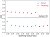 |
Fig. 7 Carbon-to-oxygen ratio (C/O) for the atmospheres of the synthetic planets. In red we plot the case in which carbon depletion is ongoing, and the carbon excess in the gas is maintained at the same abundance throughout the whole disk life. In blue we plot the case in which carbon depletion occurred in a single reset event near the beginning of the disk life. In this case the carbon excess in the gas would advect inward with the accreting gas. Included is the stellar C/O (dashed line). |
Total carbon and oxygen mass inventory from volatile gas (g), ice (i), and refractory (gr) accretion in the planetary atmosphere.
5.2.2 Super-Earths
The atmospheric C/O for the low mass planets are primarily dominated by the accretion of icy planetesimals. They tend to have lower mass atmospheres for longer, and hence incoming planetesimals tend to deposit their refractory mass directly onto the core of the planet rather than evaporate in the atmosphere. As a result, their low C/O is caused by their accretion of carbon depleted gas and oxygen rich ice after 1 Myr, driven by the surface chemistry reactions discussed earlier. We note that because of their lower masses, their global C/O may be susceptible to chemical processing of the planetary core, which we ignore.
6 Conclusions
How the astrochemisty of protoplanetary disks are imprinted into the atmospheric chemistry of exoplanets is a complex, time-dependent problem that requires a combination of detailed planet formation and disk chemistry models. Here we have combined two such models along with a new treatment of refractory carbon depletion, and its corresponding gaseous carbon excess, to compute the carbon-to-oxygen ratio (C/O) in the gas that forms the atmospheres of synthetic exoplanets.
A particularly important feature of our model is that solar system solids show signs of refractory carbon depletion relative to the carbon observed in the ISM. We argue that this missing carbon would have been released into the gas, where it is possibly available for accretion into the atmospheres of growing planets. What dictates the availability of excess carbon depends on the mechanism that produces the carbon depletion, which is currently unknown.
We posit two possible models: the reset model and the ongoing model. The first represents a catastrophic thermal event that occurred very early in the disk lifetime, while the second represents an ongoing process that is constantly producing an excess of gaseous carbon. The excess carbon from the reset model advects into the host star within 0.8 Myr, and hence is not accreted onto forming planets, while the ongoing model maintains a carbon excess in the inner (<5 AU) solar system, allowing for carbon rich (relative to solar) gas to be accreted by forming planets.
This carbon excess model is combined with the results from the chemcial evolution models by Eistrup et al. (2018) to compute the C/O distribution of the gas and solids (ice + dust) over the whole lifetime of the disk. In this evolving astrochemical disk we compute the growth and migration of planets beginning in a range of radii between 1 and 3 AU. More than half the planets end up as hot Jupiters, while the others remain super-Earth sized at radii ≥7 AU, depending on their migration histories.
In the hot Jupiters the atmospheric C/O depends on our treatment of the carbon excess model because their gas accretion is exclusively done in the region where carbon depletion is found in our solar system (volatile ices do not contribute). On the other hand, the super-Earths are more dependent on the details of the chemical model because the majority of their growth occurs outside the carbon depletion zone of the disk. For the hot Jupiters we can produce atmospheric C/O that exceeds their host star, as long as they accrete gas in the ongoing model of carbon excess. Otherwise their C/O is strictly lower than their host star because they accrete gas and solids that are both oxygen rich with respect to the host star.
We have intentionally kept the source of the carbon excess simple, studying only two possible extremes. We assumed that similar carbon depletion processes could occur in other solar systems and have not explored variance in initial C/O in both the host star and gas disk. Instead, we opted to explore what variation in C/O could occur simply from processes internal to the protoplanetary disk. Regardless we demonstrated that if the general trend of Brewer et al. (2017) holds, that most hot Jupiters have super-stellar C/O, then it is suggestive that there is a source of carbon excess in the inner parts of most stellar systems that persists throughout the lifetime of the disk or at least long enough to be incorporated into the planetary atmospheres.
Acknowledgements
Astrochemistry in Leiden is supported by the European Union A-ERC grant 291141 CHEMPLAN, by the Netherlands Research School for Astronomy (NOVA), and by a Royal Netherlands Academy of Arts and Sciences (KNAW) professor prize.
References
- Alessi, M., & Pudritz, R. E. 2018, MNRAS, 478, 2599 [NASA ADS] [CrossRef] [Google Scholar]
- Alessi, M., Pudritz, R. E., & Cridland, A. J. 2017, MNRAS, 464, 428 [NASA ADS] [CrossRef] [Google Scholar]
- Alibert, Y., Carron, F., Fortier, A., et al. 2013, A&A, 558, A109 [NASA ADS] [CrossRef] [EDP Sciences] [Google Scholar]
- Ali-Dib, M. 2017, MNRAS, 464, 4282 [NASA ADS] [CrossRef] [Google Scholar]
- Allègre, C., Manhès, G., & Lewin, É. 2001, Earth Planet. Sci. Lett., 185, 49 [NASA ADS] [CrossRef] [Google Scholar]
- Anderson, D. E., Bergin, E. A., Blake, G. A., et al. 2017, ApJ, 845, 13 [NASA ADS] [CrossRef] [Google Scholar]
- Atreya, S. K., Crida, A., Guillot, T., et al. 2016, ArXiv e-prints [arXiv:1606.04510] [Google Scholar]
- Batygin, K. 2018, AJ, 155, 178 [NASA ADS] [CrossRef] [Google Scholar]
- Bergin, E. A., Blake, G. A., Ciesla, F., Hirschmann, M. M., & Li, J. 2015, Proc. Natl. Acad. Sci., 112, 8965 [NASA ADS] [CrossRef] [Google Scholar]
- Bitsch, B., Lambrechts, M., & Johansen, A. 2015, A&A, 582, A112 [NASA ADS] [CrossRef] [EDP Sciences] [Google Scholar]
- Bitsch, B., Morbidelli, A., Johansen, A., et al. 2018, A&A, 612, A30 [NASA ADS] [CrossRef] [EDP Sciences] [Google Scholar]
- Boogert, A. C. A., Gerakines, P. A., & Whittet, D. C. B. 2015, ARA&A, 53, 541 [Google Scholar]
- Booth, R. A., Clarke, C. J., Madhusudhan, N., & Ilee, J. D. 2017, MNRAS, 469, 3994 [NASA ADS] [CrossRef] [Google Scholar]
- Bosman, A. D., Tielens, A. G. G. M., & van Dishoeck, E. F. 2018, A&A, 611, A80 [NASA ADS] [CrossRef] [EDP Sciences] [Google Scholar]
- Brewer, J. M., Fischer, D. A., & Madhusudhan, N. 2017, AJ, 153, 83 [NASA ADS] [CrossRef] [Google Scholar]
- Brouwers, M. G., Vazan, A., & Ormel, C. W. 2018, A&A, 611, A65 [NASA ADS] [CrossRef] [EDP Sciences] [Google Scholar]
- Christensen, U. R., Holzwarth, V., & Reiners, A. 2009, Nature, 457, 167 [NASA ADS] [CrossRef] [PubMed] [Google Scholar]
- Cleeves, L. I., Bergin, E. A., & Adams, F. C. 2014, ApJ, 794, 123 [NASA ADS] [CrossRef] [Google Scholar]
- Coleman, G. A. L., & Nelson, R. P. 2014, MNRAS, 445, 479 [NASA ADS] [CrossRef] [Google Scholar]
- Coleman, G. A. L., & Nelson, R. P. 2016, MNRAS, 460, 2779 [NASA ADS] [CrossRef] [Google Scholar]
- Cridland, A. J. 2018, A&A, 619, A165 [NASA ADS] [CrossRef] [EDP Sciences] [Google Scholar]
- Cridland, A. J., Pudritz, R. E., & Alessi, M. 2016, MNRAS, 461, 3274 [Google Scholar]
- Cridland, A. J., Pudritz, R. E., & Birnstiel, T. 2017a, MNRAS, 465, 3865 [NASA ADS] [CrossRef] [Google Scholar]
- Cridland, A. J., Pudritz, R. E., Birnstiel, T., Cleeves, L. I., & Bergin, E. A. 2017b, MNRAS, 469, 3910 [NASA ADS] [CrossRef] [Google Scholar]
- Cridland, A. J., Pudritz, R. E., & Alessi, M. 2019, MNRAS, 484, 345 [NASA ADS] [CrossRef] [Google Scholar]
- Dittkrist, K.-M., Mordasini, C., Klahr, H., Alibert, Y., & Henning, T. 2014, A&A, 567, A121 [NASA ADS] [CrossRef] [EDP Sciences] [Google Scholar]
- Drozdovskaya, M. N., Walsh, C., Visser, R., Harsono, D., & van Dishoeck, E. F. 2014, MNRAS, 445, 913 [NASA ADS] [CrossRef] [Google Scholar]
- Drozdovskaya,M. N., Walsh, C., van Dishoeck, E. F., et al. 2016, MNRAS, 462, 977 [NASA ADS] [CrossRef] [Google Scholar]
- Eistrup, C., Walsh, C., & van Dishoeck, E. F. 2016, A&A, 595, A83 [NASA ADS] [CrossRef] [EDP Sciences] [Google Scholar]
- Eistrup, C., Walsh, C., & van Dishoeck, E. F. 2018, A&A, 613, A14 [NASA ADS] [CrossRef] [EDP Sciences] [Google Scholar]
- Fogel, J. K. J., Bethell, T. J., Bergin, E. A., Calvet, N., & Semenov, D. 2011, ApJ, 726, 29 [NASA ADS] [CrossRef] [Google Scholar]
- Hasegawa, Y., & Pudritz, R. E. 2011, MNRAS, 417, 1236 [NASA ADS] [CrossRef] [Google Scholar]
- Hasegawa, Y., & Pudritz, R. E. 2013, ApJ, 778, 78 [NASA ADS] [CrossRef] [Google Scholar]
- Hasegawa, Y., & Pudritz, R. E. 2014, ApJ, 794, 25 [NASA ADS] [CrossRef] [Google Scholar]
- Horn, B., Lyra, W., Mac Low, M.-M., & Sándor, Z. 2012, ApJ, 750, 34 [Google Scholar]
- Ida, S., & Lin,D. N. C. 2004, ApJ, 604, 388 [NASA ADS] [CrossRef] [PubMed] [Google Scholar]
- Ida, S., & Lin,D. N. C. 2008, ApJ, 673, 487 [NASA ADS] [CrossRef] [Google Scholar]
- Ikoma, M., Nakazawa, K., & Emori, H. 2000, ApJ, 537, 1013 [NASA ADS] [CrossRef] [Google Scholar]
- Jura, M. 2008, AJ, 135, 1785 [NASA ADS] [CrossRef] [Google Scholar]
- Klarmann, L., Ormel, C. W., & Dominik, C. 2018, A&A, 618, L1 [NASA ADS] [CrossRef] [EDP Sciences] [Google Scholar]
- Kokubo, E., & Ida, S. 2002, ApJ, 581, 666 [NASA ADS] [CrossRef] [Google Scholar]
- Lambrechts, M., & Johansen, A. 2014, A&A, 572, A107 [NASA ADS] [CrossRef] [EDP Sciences] [Google Scholar]
- Lee, J.-E., Bergin, E. A., & Nomura, H. 2010, ApJ, 710, L21 [NASA ADS] [CrossRef] [Google Scholar]
- Lyra, W., Paardekooper, S.-J., & Mac Low, M.-M. 2010, ApJ, 715, L68 [NASA ADS] [CrossRef] [Google Scholar]
- Madhusudhan, N., Amin, M. A., & Kennedy, G. M. 2014, ApJ, 794, L12 [Google Scholar]
- Madhusudhan, N., Bitsch, B., Johansen, A., & Eriksson, L. 2017, MNRAS, 469, 4102 [NASA ADS] [CrossRef] [Google Scholar]
- Masset, F. S., Morbidelli, A., Crida, A., & Ferreira, J. 2006, ApJ, 642, 478 [NASA ADS] [CrossRef] [Google Scholar]
- Matsumura, S., & Pudritz, R. E. 2006, MNRAS, 365, 572 [NASA ADS] [CrossRef] [Google Scholar]
- McElroy, D., Walsh, C., Markwick, A. J., et al. 2013, A&A, 550, A36 [NASA ADS] [CrossRef] [EDP Sciences] [Google Scholar]
- Mishra, A., & Li, A. 2015, ApJ, 809, 120 [NASA ADS] [CrossRef] [Google Scholar]
- Miyake, K., & Nakagawa, Y. 1993, Icarus, 106, 20 [NASA ADS] [CrossRef] [Google Scholar]
- Morbidelli, A., Szulágyi, J., Crida, A., et al. 2014, Icarus, 232, 266 [NASA ADS] [CrossRef] [Google Scholar]
- Mordasini, C. 2013, A&A, 558, A113 [NASA ADS] [CrossRef] [EDP Sciences] [Google Scholar]
- Mordasini, C. 2014, A&A, 572, A118 [NASA ADS] [CrossRef] [EDP Sciences] [Google Scholar]
- Mordasini, C., Alibert, Y., & Benz, W. 2006, in Tenth Anniversary of 51 Peg-b: Status of and Prospects for Hot Jupiter Studies, eds. L. Arnold, F. Bouchy, & C. Moutou (Paris: Frontier Group), 84 [Google Scholar]
- Mordasini, C., Dittkrist, K.-M., Alibert, Y., et al. 2011, in The Astrophysics of Planetary Systems: Formation, Structure, and Dynamical Evolution, eds. A. Sozzetti, M. G. Lattanzi, & A. P. Boss, IAU Symp., 276, 72 [NASA ADS] [Google Scholar]
- Mordasini, C., Mollière, P., Dittkrist, K.-M., Jin, S., & Alibert, Y. 2015, Int. J. Astrobiol., 14, 201 [CrossRef] [Google Scholar]
- Mordasini, C., van Boekel, R., Mollière, P., Henning, T., & Benneke, B. 2016, ApJ, 832, 41 [NASA ADS] [CrossRef] [Google Scholar]
- Öberg, K. I., Murray-Clay, R., & Bergin, E. A. 2011, ApJ, 743, L16 [NASA ADS] [CrossRef] [Google Scholar]
- Ormel, C. W., & Klahr, H. H. 2010, A&A, 520, A43 [NASA ADS] [CrossRef] [EDP Sciences] [Google Scholar]
- Paardekooper, S.-J., Baruteau, C., & Kley, W. 2011, MNRAS, 410, 293 [NASA ADS] [CrossRef] [Google Scholar]
- Pinilla, P., Klarmann, L., Birnstiel, T., et al. 2016, A&A, 585, A35 [NASA ADS] [CrossRef] [EDP Sciences] [Google Scholar]
- Pollack, J. B., Hubickyj, O., Bodenheimer, P., et al. 1996, Icarus, 124, 62 [NASA ADS] [CrossRef] [Google Scholar]
- Pontoppidan, K. M., Salyk, C., Bergin, E. A., et al. 2014, Protostars and Planets VI (Tucson, AZ: University of Arizona Press), 363 [Google Scholar]
- Raettig, N., Klahr, H., & Lyra, W. 2015, ApJ, 804, 35 [NASA ADS] [CrossRef] [Google Scholar]
- Schäfer, U., Yang, C.-C., & Johansen, A. 2017, A&A, 597, A69 [NASA ADS] [CrossRef] [EDP Sciences] [Google Scholar]
- Schlichting, H. E., Sari, R., & Yalinewich, A. 2015, Icarus, 247, 81 [NASA ADS] [CrossRef] [Google Scholar]
- Shakura, N. I., & Sunyaev, R. A. 1973, A&A, 24, 337 [NASA ADS] [Google Scholar]
- Szulágyi, J., Morbidelli, A., Crida, A., & Masset, F. 2014, ApJ, 782, 65 [NASA ADS] [CrossRef] [Google Scholar]
- Thiabaud, A., Marboeuf, U., Alibert, Y., Leya, I., & Mezger, K. 2015, A&A, 574, A138 [NASA ADS] [CrossRef] [EDP Sciences] [Google Scholar]
- Visser, R., van Dishoeck, E. F., Doty, S. D., & Dullemond, C. P. 2009, A&A, 495, 881 [NASA ADS] [CrossRef] [EDP Sciences] [Google Scholar]
- Visser, R., Doty, S. D., & van Dishoeck, E. F. 2011, A&A, 534, A132 [NASA ADS] [CrossRef] [EDP Sciences] [Google Scholar]
- Walsh, C., Nomura, H., & van Dishoeck, E. 2015, A&A, 582, A88 [NASA ADS] [CrossRef] [EDP Sciences] [Google Scholar]
- Weidenschilling, S. J. 1977, MNRAS, 180, 57 [NASA ADS] [CrossRef] [Google Scholar]
- Whittet, D. C. B., Poteet, C. A., Chiar, J. E., et al. 2013, ApJ, 774, 102 [NASA ADS] [CrossRef] [Google Scholar]
Radial drift is a known physical process that brings dust into the inner disk faster than viscous evolution. So in principle the Sun has accreted material with a lower gas-to-dust mass ratio than 100. Low gas-to-dust ratios would lead to large estimates of ndust and hence larger elemental abundances in refractories
All Tables
Carbon-to-hydrogen (C/H) and carbon-to-oxygen (C/O) ratios for the volatiles (gas), refractories (gr), and combined (tot) given the simple model (mdl) where dust mass is dominated by enstatite and solid carbon (with C/Si = 6).
Total carbon and oxygen mass inventory from volatile gas (g), ice (i), and refractory (gr) accretion in the planetary atmosphere.
All Figures
|
Fig. 1 Radial dependency of carbon depletion as described in Eq. (3). The inset shows the same plot in log-space, mimicking Fig. 2 of Mordasini et al. (2016). |
| In the text | |
|
Fig. 2 Available excess carbon for atmospheric accretion. We assume that in the ongoing model the excess carbon is supplied by ongoing processing of dust grains, delivering the carbon to the gas. In the reset model the carbon excess is generated early in the disk life and advects with the bulk gas into the host star. |
| In the text | |
|
Fig. 3 Evolution of C/O in gas (left) and ice (right) from Eistrup et al. (2018). We note the location of the water (solid), CO2 (dashed), O2 (dotted), and CO (dot-dashed) ice lines. A step-function in C/O is seen early on in the disk’s life, which becomes complicated by chemistry as the disk ages. After ~ Myr CO is converted into frozen CO2 outward of the CO2 ice line, which lowers the gas C/O while raising the ice C/O, eventually becoming more carbon rich than the gas. |
| In the text | |
|
Fig. 4 Planet formation tracks for the synthetic planets formed in this work. There is an easily distinguishable bifurcation between the orbital evolution of the planets caused by their interaction with the disk. |
| In the text | |
|
Fig. 5 Combined torque maps and planet formation tracks for four different snapshots throughout the formation history of our three planets of interest. In the torque maps (colored region) red denotes inward migration, white denotes zero net torque, and blue denotes outward migration. The band of outward migration between 1 and 10 AU is caused by our choice of disk model and the opacity arising from CO2 freeze out. |
| In the text | |
|
Fig. 6 Similar to Fig. 3, but including the effect of the excess gaseous carbon caused by the reset scenario of carbon depletion. The carbon advects inward quickly, disappearing before 1 Myr. The ongoing scenario would maintain the same level of carbon excess over the lifetime of the disk. Additionally we overplot the radial evolution of the three targeted planets. The dots along each track denote thepoint at which (starting from the bottom) the planet begins accreting gas, when it has accreted 3 M⊕ of gas, and when the planet has reached half of its final mass. The inner two planets accrete their gas primarily within the ice line, while the outer planet accretes its gas between the CO2 and CO ice lines. |
| In the text | |
|
Fig. 7 Carbon-to-oxygen ratio (C/O) for the atmospheres of the synthetic planets. In red we plot the case in which carbon depletion is ongoing, and the carbon excess in the gas is maintained at the same abundance throughout the whole disk life. In blue we plot the case in which carbon depletion occurred in a single reset event near the beginning of the disk life. In this case the carbon excess in the gas would advect inward with the accreting gas. Included is the stellar C/O (dashed line). |
| In the text | |
Current usage metrics show cumulative count of Article Views (full-text article views including HTML views, PDF and ePub downloads, according to the available data) and Abstracts Views on Vision4Press platform.
Data correspond to usage on the plateform after 2015. The current usage metrics is available 48-96 hours after online publication and is updated daily on week days.
Initial download of the metrics may take a while.