| Issue |
A&A
Volume 627, July 2019
|
|
|---|---|---|
| Article Number | A156 | |
| Number of page(s) | 7 | |
| Section | Numerical methods and codes | |
| DOI | https://doi.org/10.1051/0004-6361/201730557 | |
| Published online | 16 July 2019 | |
Polarimetric imaging of circumstellar disks
I. Artifacts due to limited angular resolution
Leiden Observatory, Leiden University, PO Box 9513, 2300 RA Leiden, The Netherlands
e-mail: This email address is being protected from spambots. You need JavaScript enabled to view it.
Received:
3
February
2017
Accepted:
28
February
2019
Abstract
Context. Polarimetric images of circumstellar environments, even when corrected with adaptive optics, have a limited angular resolution. Finite resolution greatly affects polarimetric images because of the canceling of adjacent polarization signals with opposite signs. In radio astronomy this effect is called beam depolarization and is well known. However, radio techniques to mitigate beam depolarization are not directly applicable to optical images as a consequence of the inherent lack of phase information at optical wavelengths.
Aims. We explore the effects of a finite point-spread function (PSF) on polarimetric images and the application of Richardson-Lucy deconvolution to polarimetric images.
Methods. We simulated polarimetric images of highly simplified, circumstellar disk models and convolved these with simulated and actual SPHERE/ZIMPOL PSFs. We attempted to deconvolve simulated images in orthogonal linear polarizations and polarized intensity images.
Results. The most significant effect of finite angular resolution is the loss of polarimetric signal close to the central star where large polarization signals of opposite signs average out. The finite angular resolution can also introduce polarized light in areas beyond the original, polarized signal such as outside of disks. These effects are particularly severe for disks that are not rotationally symmetric. The deconvolution of polarimetric images is far from trivial. Richardson-Lucy deconvolution applied to images in opposite linear polarization states, which are subsequently subtracted from each other, cannot recover the signal close to the star. Sources that lack rotational symmetry cannot be recovered with this deconvolution approach.
Key words: polarization / methods: numerical / techniques: polarimetric / techniques: image processing
© ESO 2019
1. Introduction
To understand the evolution of planetary systems from dust to planets we need to observe circumstellar disks around other stars. The observations of different circumstellar systems can provide us with information of how and where planets form in disks. There are a myriad of systems each with different structures such as multiple rings, gaps, and even spiral arms (Avenhaus et al. 2014; Pohl et al. 2017). Many of the structures expected from planet-disk interactions occur on very small scales. Observations of light scattered by dust grains in disks are an excellent approach to detect disk structures at high angular resolution. Since the scattered light is polarized, it can be easily distinguished from starlight using polarimetric imaging.
Over the last few years polarimetric imaging of circumstellar disks at visible and near-infrared wavelengths has made great progress in terms of angular resolution and polarimetric sensitivity. High-contrast imagers for the direct imaging of circumstellar disks and exoplanets often include polarimetric imaging capabilities because polarization easily differentiates between the unpolarized starlight and polarized scattered light from dust and planetary atmospheres and surfaces (Kuhn et al. 2001; Apai et al. 2003; Rodenhuis et al. 2012). In particular the Gemini Planet Imager (GPI; Macintosh et al. 2014) and Spectro-Polarimetric High-contrast Exoplanet REsearch (SPHERE; Beuzit et al. 2008) combine extreme adaptive optics (AO), coronagraphs, and imaging polarimeters. Both instruments measure two orthogonal linear polarization states simultaneously (Perrin et al. 2015) or almost simultaneously (Thalmann et al. 2008), thereby providing high-quality polarimetric images.
GPI and the Infrared Dual-band Imager and Spectrograph (IRDIS) of SPHERE achieve high Strehl ratios at near-infrared wavelengths for bright targets (Poyneer et al. 2014; Fusco et al. 2006). Observations at visible wavelengths with the Zurich Imaging Polarimeter (ZIMPOL) of SPHERE, even for bright targets, and observations with GPI and SPHERE/IRDIS in the near-infrared for faint targets suffer from limited Strehl ratios, resulting in a significant smearing of the polarimetric image. The Strehl ratio for SPHERE/ZIMPOL approaches 60% for the brightest targets and decreases for fainter targets; for magnitude 12 and greater the Strehl ratio is less than 10% (SPHERE User Manual P97.2). Even under the most favorable atmospheric conditions and for bright targets, the point-spread function (PSF) can be far from ideal due to the so-called low wind effect (Sauvage et al. 2015).
The PSF of an image that has been corrected by an extreme AO system consists of a diffraction-limited core with a peak intensity of S, the Strehl ratio. Outside of the diffraction-limited core, 1 − S of the intensity is smeared over a disk with a radius of r0(λ)/D, where r0 is the Fried parameter at the relevant wavelength λ, and D is the telescope diameter. For intensity images that are always positive, the convolution with an AO-corrected PSF leads to a sharp image on top of a relatively smooth background. The influence of such a PSF is markedly different for polarimetric images, which contain positive and negative signals. These signals with opposite sign cancel each other in the center of the image as a consequence of smearing by the PSF. This instrumental depolarization is due to the combined PSF of the atmosphere, telescope, and instrument. This cancelation of polarization signals is similar to the widely known beam depolarization in radio observations. This depolarization occurs when magnetized plasma between the source and observer changes the polarization signal emitted by a source on angular scales smaller than the beam width (Tribble 1991; Haverkorn & Heitsch 2004).
In this paper we study the effects of limited angular resolution on polarimetric images by convolving simulated polarized images of circumstellar disk models with simulated and observed PSFs. Section 2 shows educational examples of how a PSF can affect a polarimetric image. In Sect. 3 we explore whether deconvolution can retrieve the original polarization signal by applying a Richardson-Lucy (RL) deconvolution to intensity images in orthogonal linear polarization states and to polarized intensity images. We discuss this deconvolution approach in Sect. 4.
2. Influence of finite PSF on polarimetric images
To study the influence of limited angular resolution on polarimetric images, we convolved two simulated sources with a simulated PSF and an actual SPHERE/ZIMPOL PSF in the R and I bands. The two simulated sources are a uniform, face-on disk and a partially obscured disk. Section 2.1 describes the disk models and Sects. 2.2 and 2.3 describe the effects of a Gaussian PSF and SPHERE/ZIMPOL PSFs, respectively.
2.1. Face-on disk and obscured disk models
We assume that the circumstellar disk is seen in scattered starlight where a photon is only scattered once (single-scattering approximation). We further assume that the scattered light becomes 100% linearly polarized with an angle of linear polarization that is orthogonal to the radius vector. While actual scattering mechanisms do not completely polarize the scattered light, the following simulations and analyses are independent of the overall degree of linear polarization. The observed light from a uniform, face-on circumstellar disk with outer radius rdisk is then given by
 (1)
(1)
 (2)
(2)
 (3)
(3)
The quantity I is the intensity of the scattered light, which drops off as 1/r2 to account for the decrease in starlight with radius r, θ is the azimuth of the polar coordinate system with the star at its origin, and Q and U are the two Stokes vector components that describe linearly polarized light.
Using these equations we simulated two highly idealized, polarized sources: a uniform, face-on disk as shown in Fig. 1 and a partially obscured face-on disk shown in Fig. 2, to reduce the high dynamic range in the disk images it is common to scale the images with r2. The obscured disk is the upper half of the uniform disk. Since we define the center of a pixel as the center of our coordinate system, the horizontal row of pixels going through the origin only contains half of the signal in the full-disk model. This ensures that the sum of all polarization signals is zero. While this model of a partially obscured disk is rather unrealistic, its simplicity and relation to the rotationally symmetric face-on disk model makes it ideal to showcase the issues arising from a lack of symmetry.
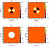 |
Fig. 1. Simulated images of a uniform, face-on disk in Q, U, Qϕ, and Uϕ. All images are scaled with r2 owing to the high dynamic range created by the intensity drop-off. We note that the scale goes to ±100; we multiplied the intensity value from Eq. (1) by 100. |
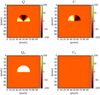 |
Fig. 2. Model of a partially obscured polarized disk in Q, U, Qϕ, and Uϕ. All images are scaled with r2 owing to the high dynamic range created by the intensity drop-off. We note that the scale goes to ±100; we multiplied the intensity value from Eq. (1) by 100. |
Polarimetric images of circumstellar environments are often shown in terms of Qϕ and Uϕ (Quanz et al. 2013), which are defined as
 (4)
(4)
 (5)
(5)
Single scattering polarization is tangential to the radius vector between the star and scatterer. Therefore Uϕ is expected to vanish for single scattering, and Qϕ is a measure of the amount of polarized light that has been scattered. By assuming that Uϕ = 0, depolarization, and instrumental polarization induced by the telescope and instrument can be disentangled from the actual polarization signal (Avenhaus et al. 2014).
While Eqs. (4) and (5) seem to be linear at first sight, they actually present a nonlinear transformation of the linear polarization coordinate system. Similarly the degree of linear polarization  is also nonlinear with respect to the Stokes parameters Q and U. Because of these nonlinearities, the influence of a finite PSF is not immediately obvious.
2.2. Convolution with Gaussian PSF
To showcase the effect of limited angular resolution on polarimetric images of circumstellar disks, we used a Gaussian PSF with a full width at half maximum (FWHM) of 20 pixels; in comparison, the face-on disk diameter is twice as large as the PSF FWHM. The cross section of the Gaussian PSF is shown in Fig. 5. We did not add noise to these simulations to emphasize the effect of the convolution as compared to other effects that may occur due to noise. The convolution of the disk models with the Gaussian PSF are shown in Figs. 3 and 4 where the top rows show Stokes Q and U, and the bottom rows show Qϕ and Uϕ, where Qϕ and Uϕ are calculated from the convolved Q and U with the PSF.
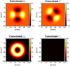 |
Fig. 3. Q, U, Qϕ and Uϕ of the uniform, face-on disk convolved with the Gaussian PSF. All images are scaled with r2 due to the high dynamic range created by the intensity drop-off. |
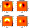 |
Fig. 4. Values Q, U, Qϕ, and Uϕ of the partially obscured disk convolved with the Gaussian PSF. All images are scaled with r2 owing to the high dynamic range created by the intensity drop-off. |
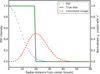 |
Fig. 5. Educational example of PSF depolarization on convolved images due to simulated Gaussian PSF. The cross section of the uniform disk as shown in Fig. 1 and Qϕ of the convolved disk as shown in Fig. 3. Solid green line: true disk polarization; red dotted line: Qϕ of the convolved disk; blue, dashed line: the Gaussian PSF. |
The convolved image shows a larger disk with an inner hole. The comparison of cross sections in Fig. 5 shows that the signal completely disappears at the center; polarized flux is found beyond the original disk radius and even extends beyond the FWHM of the PSF. Both the apparent lack of polarized flux at the center and the substantial extension in the apparent disk radius are due to the finite extent of the PSF and the presence of both positive and negative signals in Q and U. The value Uϕ remains zero even after the convolution with the PSF in this particular case with complete azimuthal symmetry.
Sources without azimuthal symmetry such as the obscured disk described above also suffer from the convolution with the PSF to the point where the convolved source has little resemblance with the original source (see Fig. 4). After the convolution, the orientation of the linear polarization is no longer tangential to the radius vector. The quantity Qϕ even turns negative in the lower half where the model has no signal at all. The value Uϕ is comparable in magnitude to Qϕ and does not vanish as in the case of the face-on disk that is rotationally symmetric and uniform.
At first sight the nonzero Uϕ of the convolved image might be surprising as all equations are linear. However, Eqs. (1)–(3) have a spatially varying linear coefficient, which depends on the azimuth. Therefore Qϕ and Uϕ of the convolved data are not the same as the convolution of the true Qϕ and Uϕ with the PSF. In the case of Uϕ, the convolution with the PSF can create a Uϕ signal if the object deviates from rotational symmetry.
2.3. Convolution with SPHERE/ZIMPOL PSF
We conclude our simulations with a real SPHERE/ZIMPOL PSF, an intensity image of the mV = 11.4 reference star TYC 5259-446-1. The simultaneously observed R and I band PSFs have Strehl ratios of 2.8% and 6.8%, respectively and the FWHMs are 18 pixels or 50 mas and 14 pixels or 40 mas, respectively. Both PSFs show deviation from rotational symmetry. Figure 7 shows the azimuthally averaged PSF in R band.
The convolution of the uniform, face-on disk model and the partially obscured face-on disk model with the SPHERE/ZIMPOL PSF in R band are shown in Fig. 6. As expected, the polarized flux in the convolved Qϕ image is strongly suppressed in the center. This is also evident in Fig. 7, which shows the cross section of the convolved Qϕ image along with the original source model. For the partially obscured disk, the convolution with the PSF destroys the azimuthal symmetry of the original source.
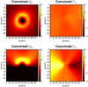 |
Fig. 6. Top row: Qϕ and Uϕ images of the uniform disk convolved with the SPHERE/ZIMPOL reference PSF in R band. Bottom row: Qϕ and Uϕ images of the partially obscured disk convolved with the SPHERE/ZIMPOL reference PSF in R band. All images are scaled with r2 owing to the high dynamic range created by the intensity drop-off. |
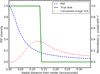 |
Fig. 7. Educational example of PSF depolarization on convolved images due to a reference SPHERE/ZIMPOL PSF. The cross sections of uniform, face-on disk. Green, solid line: the original polarized disk signal. Blue, dashed line: the SPHERE/ZIMPOL PSF in R band as shown in Fig. 6. Red dotted line: the polarization signal after convolution with the SPHERE/ZIMPOL PSF in R band. |
2.4. Effects of finite PSF on intensity images
Intensity images are also affected by the convolution with the PSF and show a marked loss of signal at disk center, in addition to the general smearing expected from a finite PSF. The intensity of our uniform, face-on disk drops off with 1/r2; when scaled with r2, as is usual when showing disk images, the r2 signal is constant within the disk radius. After convolution with a Gaussian PSF, the disk signal is smeared and exhibits a central hole when scaled with r2 (see Fig. 8): the larger the FWHM of the PSF, the larger the size of the apparent central hole.
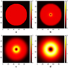 |
Fig. 8. Intensity images of the uniform, face-on disk scaled with r2. Original disk model (a), original disk model convolved with a Gaussian PSF with a FWHM of 2 pixels (b), 5 pixels (c), and 10 pixels (d). |
3. Deconvolution
The previous section showed that the effect of limited angular resolution on polarimetric images goes far beyond a simple smearing of the true polarization signal. The question arises whether a deconvolution algorithm could restore the original polarization signal. The convolution of the PSF with the source image can create asymmetry in the Qϕ and Uϕ signals. To remove the PSF and noise signal from the observed signal the deconvolution needs to take place in the Q and U frame as a consequence of the nonlinear transformation between Q and Qϕ and U and Uϕ as shown in Eqs. (4) and (5). In this section we explore deconvolutions of Q and U; we also study the deconvolution of PL to assess the effects of deconvolving a quantity that is nonlinear in Q and U.
Deconvolution is used to mitigate noise and PSF smearing in observed images. Intensity images that are affected by broad PSF wings can profit from deconvolution to improve the angular resolution. Many deconvolution algorithms have been developed and applied successfully to a variety of problems, for example, Starck et al. (2002). In astronomy, RL deconvolution (Richardson 1972; Lucy 1974) is frequently used and is based on Bayes theorm, Poisson noise, and the non-negativity of the true signal. The RL deconvolution approach maximizes the likelihood of a deconvolved image (Starck et al. 2002; McLean 2008) using the following iterative equation:
 (6)
(6)
where again O is the deconvolved image, I are the observed data, and P is the normalized PSF. Several authors have published deconvolved polarimetric images including L2 Puppis and Betelgeuse, where polarized images have been deconvolved with the RL technique (Kervella et al. 2015, 2016). In the infrared this technique was applied by Potter et al. (1999) and Rauch et al. (2013). We used our simulated observations to assess the validity of using standard RL deconvolution to polarized data sets.
Since RL enforces non-negativity of the deconvolved image, this technique cannot be applied directly to images such as Stokes Q and U. We therefore deconvolve intensity images in opposite polarization states and the polarized intensity, which is also a positive quantity. Our aim is not to resolve disk structures smaller than the core of the PSF, which is difficult to achieve as demonstrated by Lucy (1992).
3.1. Richardson-Lucy deconvolution of polarization images
Stokes Q and U are not directly observed, but intensity images I + Q, I − Q, I + U, I − U are directly observable quantities. The directly observed images are therefore non-negative and can be deconvolved. After deconvolution, estimates of the true source polarization signal, Q′ and U′, can be obtained from
![Mathematical equation: $$ \begin{aligned} Q=(\text {\DH } [I+Q]-\text {\DH } [I-Q] ) /2, \end{aligned} $$](/articles/aa/full_html/2019/07/aa30557-17/aa30557-17-eq8.gif) (7)
(7)
![Mathematical equation: $$ \begin{aligned} U=(\text {\DH } [I+U]-\text {\DH } [I-U] ) /2, \end{aligned} $$](/articles/aa/full_html/2019/07/aa30557-17/aa30557-17-eq9.gif) (8)
(8)
where Ð stands for the deconvolution. The quantities  and
and  can then be calculated from Q′ and U′ using Eqs. (4) and (5). Since the deconvolution is a nonlinear process, Q′ and U′ are not necessarily adequate estimates of the actual source polarization.
Another non-negative polarization quantity derived from the observations is the polarized intensity  . Deconvolution of the polarized intensity might seem like an attractive solution as the intensity is no longer involved. However, the nonlinear nature of the polarized intensity with respect to the observed quantities poses a problem. As such there is no obvious solution to the lack of non-negative quantities in polarimetric imaging. In the following we explore the effectiveness of these two deconvolution approaches using our uniform, face-on disk, and obscured disk models.
3.2. Deconvolution results
The results of RL deconvolving the intensity images for the models convolved with the Gaussian PSF are shown in Figs. 9 and 10. The quantity Uϕ is not shown for the uniform disk deconvolution because the deconvolved Uϕ signal is very small. While the deconvolved Qϕ images look sharper, the central hole remains. Similarly for the partially obscured disk, both Qϕ and Uϕ become sharper but the deconvolution does not retrieve the original structure. In the case of the SPHERE/ZIMPOL PSF case (Figs. 11 and 12), the uniform disk shows signals in both Qϕ and Uϕ because the reference PSF is not symmetrical, which results in a finite Uϕ signal. The deconvolution sharpens the observed structure, and for the partially obscured disk it does not decrease the Uϕ signal. Deconvolution of the intensity images generally sharpens the features seen in the convolved images and the diameter of the deconvolved disk decreases. A nonphysical signal is still present after deconvolution of the intensity images. The RL deconvolution does reduce some artifacts but does not recover the original structure.
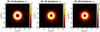 |
Fig. 9. Deconvolution of intensity images of the uniform disk convolved with the Gaussian PSF. The deconvolved Qϕ images are shown after 10, 50, and 80 iterations; Uϕ is not shown because of the small signal levels. All images are scaled with r2 owing to the high dynamic range created by the intensity drop-off. |
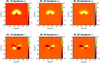 |
Fig. 10. Deconvolution of intensity images of the partially obscured disk convolved with the Gaussian PSF. The deconvolved Qϕ and Uϕ images are shown after 10, 50, and 80 iterations. All images are scaled with r2 owing to the high dynamic range created by the intensity drop-off. |
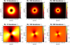 |
Fig. 11. Deconvolution of intensity images of the uniform disk convolved with the SPHERE/ZIMPOL PSF. The deconvolved Qϕ and Uϕ images are shown after 10, 100, and 500 iterations. All images are scaled with r2 owing to the high dynamic range created by the intensity drop-off. |
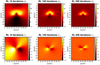 |
Fig. 12. Deconvolution of intensity images of the partially obscured polarized disk convolved with the SPHERE/ZIMPOL PSF. The deconvolved Qϕ and Uϕ images are shown after 10, 100, and 500 iterations. All images are scaled with r2 owing to the high dynamic range created by the intensity drop-off. |
Deconvolution of the linearly polarized intensity pL leads to rather different results (Figs. 13 and 14). The disk diameter does not decrease with an increase in iterations but the signal is reduced into a small ring. The uniform disk model convolved with the Gaussian PSF and the SPHERE/ZIMPOL I-band PSF show similar results. The inner hole becomes larger and the ring becomes sharper. The most apparent difference between PSFs occurs for the partially obscured disk. For the Gaussian PSF, the polarized intensity shows a ring-like structure that the deconvolution decreases in size. Almost half of the deconvolved signals appears in the lower half where the original source has no signal at all. For the sharper SPHERE/ZIMPOL PSF, the deconvolved signal is largely confined to the area of the original signal, although the inner hole persists. This dependence on the PSF shape happens because the polarized intensity is not a linear combination of directly observed quantities. The deconvolution of the polarized intensity sharpens the image, but does not recover the polarization signal lost by averaging over close-by polarization signals with opposite sign and may even introduce artificial structures that are not present in the original source.
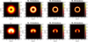 |
Fig. 13. Deconvolution of the polarized intensity of uniform disk and partially obscured disk convolved with the Gaussian PSF. The convolved image and deconvolved images are shown after 10, 50, and 80 iterations. All images are scaled with r2 owing to the high dynamic range created by the intensity drop-off. |
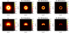 |
Fig. 14. Deconvolution of the polarized intensity of uniform disk and partially obscured disk convolved with the SPHERE/ZIMPOL reference PSF. The convolved image and deconvolved images are shown after 10, 100, and 500 iterations. All images are scaled with r2 owing to the high dynamic range created by the intensity drop-off. |
Both the RL deconvolution of the intensity images and the polarized intensity reduce the size of features. In case of the polarized intensity, a single image is deconvolved, which generally sharpens the structures seen in the convolved polarized intensity without reducing the diameter of the features. In contrast, RL deconvolution of the intensity images I + Q, I − Q, I + U, and I − U simply reduces the diameter of the features because these images are dominated by the intensity and the deconvolved images have most of their signal very close to the center. The resulting Q and U images are therefore scaled versions of the convolved features. In summary, both deconvolution approaches result in deconvolved images that often have little resemblance with the original structure.
One might wonder whether the RL deconvolution would converge to the correct result if the number of iterations were increased; we have never observed that. There is no substantial change in terms of the observed artifacts in the deconvolved images after about 100 iterations. This is not surprising since PL is not linear in Q and U; also RL deconvolution is nonlinear, which implies that the difference between the deconvolved I + Q and I − Q images is not the same as the deconvolution of Q itself.
4. Discussion
We have shown that the limited angular resolution of images in polarized light can introduce artifacts that go far beyond a simple smearing. In particular linear polarization observations of circumstellar disks displayed in terms of Qϕ and Uϕ are easily misinterpreted. Limited angular resolution leads to three types of artifacts in observations of circumstellar disks: (1) the apparent outer disk radius is determined by the extension of the PSF halo given by the ratio of λ/r0, unless the true disk size is much larger than the PSF; (2) the depolarization close to the center of the disk is due to the proximity of positive and negative polarization signals that cancel each other when observed with limited angular resolution and therefore, polarimetric images of circumstellar disks always have a hole in the center even if that is not really the case and (3) if either the source or the PSF lack rotational symmetry, the polarization of the convolved image is no longer confined to the azimuthal direction, and a finite signal in Uϕ can be due to the limited resolution, which may be confused with effects due to multiple scattering (Canovas et al. 2015) or instrumental polarization (Avenhaus et al. 2014). Moreover, limited angular resolution on only intensity images results in the peak flux levels of the observed source leveling out, which also creates a gap in the center of the disk that is emphasized by r2 scaling.
The RL deconvolution and subsequent subtraction of the observed I + Q, I − Q, I + U and I − U images does not recover the original source signal. Deconvolving the polarized intensity does not recover the original signal either and can create a narrow ring in the case of a uniform, face-on disk. In conclusion, none of these deconvolution approaches are able to recover even the most simple of structures.
If comparisons of observations with models are made, the models should always be convolved with the observed PSF instead of trying to deconvolve polarized images. This is particularly important when trying to estimate the disk brightness close to the star and the extension of the disk.
Acknowledgments
We thank Jos de Boer for the TYC 5259-446-1 dataset.
References
- Apai, D., Brandner, W., Pascucci, I., et al. 2003, in Earths: DARWIN/TPF and the Search for Extrasolar Terrestrial Planets, eds. M. Fridlund, T. Henning, & H. Lacoste, ESA SP, 539, 329 [NASA ADS] [Google Scholar]
- Avenhaus, H., Quanz, S. P., Schmid, H. M., et al. 2014, ApJ, 781, 87 [NASA ADS] [CrossRef] [Google Scholar]
- Beuzit, J. L., Feldt, M., Dohlen, K., et al. 2008, Proc. SPIE, 7014, 18 [Google Scholar]
- Canovas, H., Ménard, F., de Boer, J., et al. 2015, A&A, 582, L7 [NASA ADS] [CrossRef] [EDP Sciences] [Google Scholar]
- Fusco, T., Rousset, G., Sauvage, J.-F., et al. 2006, Opt. Exp., 14, 7515 [Google Scholar]
- Haverkorn, M., & Heitsch, F. 2004, A&A, 421, 1011 [NASA ADS] [CrossRef] [EDP Sciences] [Google Scholar]
- Kervella, P., Montargès, M., & Lagadec, E. 2015, EAS Pub. Ser., 71, 211 [CrossRef] [Google Scholar]
- Kervella, P., Lagadec, E., Montargès, M., et al. 2016, A&A, 585, A28 [NASA ADS] [CrossRef] [EDP Sciences] [Google Scholar]
- Kuhn, J. R., Potter, D., & Parise, B. 2001, ApJ, 553, L189 [NASA ADS] [CrossRef] [Google Scholar]
- Lucy, L. B. 1974, AJ, 79, 745 [NASA ADS] [CrossRef] [Google Scholar]
- Lucy, L. B. 1992, AJ, 104, 1260 [NASA ADS] [CrossRef] [Google Scholar]
- Macintosh, B., Graham, J. R., Ingraham, P., et al. 2014, Proc. Nat. Acad. Sci., 111, 12661 [Google Scholar]
- McLean, I. S. 2008, Electronic Imaging in Astronomy (Springer) [Google Scholar]
- Perrin, M. D., Duchene, G., Millar-Blanchaer, M., et al. 2015, ApJ, 799, 182 [Google Scholar]
- Pohl, A., Benisty, M., Pinilla, P., et al. 2017, ApJ, 850, 52 [NASA ADS] [CrossRef] [Google Scholar]
- Potter, D. E., Close, L. M., Roddier, F., et al. 1999, in European Southern Observatory Conference and Workshop Proceedings, ed. D. Bonaccini, 56, 353 [Google Scholar]
- Poyneer, L. A., De Rosa, R. J., Macintosh, B., et al. 2014, Proc. SPIE, 91480K [Google Scholar]
- Quanz, S. P., Avenhaus, H., Buenzli, E., et al. 2013, ApJ, 766, L2 [NASA ADS] [CrossRef] [Google Scholar]
- Rauch, C., Mužić, K., Eckart, A., et al. 2013, A&A, 551, A35 [NASA ADS] [CrossRef] [EDP Sciences] [Google Scholar]
- Richardson, W. H. 1972, J. Opt. Soc. Am. (1917–1983), 62, 55 [Google Scholar]
- Rodenhuis, M., Canovas, H., Jeffers, S. V., et al. 2012, Proc. SPIE, 8446, 9 [Google Scholar]
- Sauvage, J. F., Fusco, T., Guesalaga, A., et al. 2015, Adaptive Optics for Extremely Large Telescopes 4 – Conference Proceedings [Google Scholar]
- Starck, J. L., Pantin, E., & Murtagh, F. 2002, PASP, 114, 1051 [NASA ADS] [CrossRef] [Google Scholar]
- Thalmann, C., Schmid, H. M., Boccaletti, A., et al. 2008, Proc. SPIE, 7014, 3 [Google Scholar]
- Tribble, P. C. 1991, MNRAS, 250, 726 [NASA ADS] [CrossRef] [Google Scholar]
All Figures
|
Fig. 1. Simulated images of a uniform, face-on disk in Q, U, Qϕ, and Uϕ. All images are scaled with r2 owing to the high dynamic range created by the intensity drop-off. We note that the scale goes to ±100; we multiplied the intensity value from Eq. (1) by 100. |
| In the text | |
|
Fig. 2. Model of a partially obscured polarized disk in Q, U, Qϕ, and Uϕ. All images are scaled with r2 owing to the high dynamic range created by the intensity drop-off. We note that the scale goes to ±100; we multiplied the intensity value from Eq. (1) by 100. |
| In the text | |
|
Fig. 3. Q, U, Qϕ and Uϕ of the uniform, face-on disk convolved with the Gaussian PSF. All images are scaled with r2 due to the high dynamic range created by the intensity drop-off. |
| In the text | |
|
Fig. 4. Values Q, U, Qϕ, and Uϕ of the partially obscured disk convolved with the Gaussian PSF. All images are scaled with r2 owing to the high dynamic range created by the intensity drop-off. |
| In the text | |
|
Fig. 5. Educational example of PSF depolarization on convolved images due to simulated Gaussian PSF. The cross section of the uniform disk as shown in Fig. 1 and Qϕ of the convolved disk as shown in Fig. 3. Solid green line: true disk polarization; red dotted line: Qϕ of the convolved disk; blue, dashed line: the Gaussian PSF. |
| In the text | |
|
Fig. 6. Top row: Qϕ and Uϕ images of the uniform disk convolved with the SPHERE/ZIMPOL reference PSF in R band. Bottom row: Qϕ and Uϕ images of the partially obscured disk convolved with the SPHERE/ZIMPOL reference PSF in R band. All images are scaled with r2 owing to the high dynamic range created by the intensity drop-off. |
| In the text | |
|
Fig. 7. Educational example of PSF depolarization on convolved images due to a reference SPHERE/ZIMPOL PSF. The cross sections of uniform, face-on disk. Green, solid line: the original polarized disk signal. Blue, dashed line: the SPHERE/ZIMPOL PSF in R band as shown in Fig. 6. Red dotted line: the polarization signal after convolution with the SPHERE/ZIMPOL PSF in R band. |
| In the text | |
|
Fig. 8. Intensity images of the uniform, face-on disk scaled with r2. Original disk model (a), original disk model convolved with a Gaussian PSF with a FWHM of 2 pixels (b), 5 pixels (c), and 10 pixels (d). |
| In the text | |
|
Fig. 9. Deconvolution of intensity images of the uniform disk convolved with the Gaussian PSF. The deconvolved Qϕ images are shown after 10, 50, and 80 iterations; Uϕ is not shown because of the small signal levels. All images are scaled with r2 owing to the high dynamic range created by the intensity drop-off. |
| In the text | |
|
Fig. 10. Deconvolution of intensity images of the partially obscured disk convolved with the Gaussian PSF. The deconvolved Qϕ and Uϕ images are shown after 10, 50, and 80 iterations. All images are scaled with r2 owing to the high dynamic range created by the intensity drop-off. |
| In the text | |
|
Fig. 11. Deconvolution of intensity images of the uniform disk convolved with the SPHERE/ZIMPOL PSF. The deconvolved Qϕ and Uϕ images are shown after 10, 100, and 500 iterations. All images are scaled with r2 owing to the high dynamic range created by the intensity drop-off. |
| In the text | |
|
Fig. 12. Deconvolution of intensity images of the partially obscured polarized disk convolved with the SPHERE/ZIMPOL PSF. The deconvolved Qϕ and Uϕ images are shown after 10, 100, and 500 iterations. All images are scaled with r2 owing to the high dynamic range created by the intensity drop-off. |
| In the text | |
|
Fig. 13. Deconvolution of the polarized intensity of uniform disk and partially obscured disk convolved with the Gaussian PSF. The convolved image and deconvolved images are shown after 10, 50, and 80 iterations. All images are scaled with r2 owing to the high dynamic range created by the intensity drop-off. |
| In the text | |
|
Fig. 14. Deconvolution of the polarized intensity of uniform disk and partially obscured disk convolved with the SPHERE/ZIMPOL reference PSF. The convolved image and deconvolved images are shown after 10, 100, and 500 iterations. All images are scaled with r2 owing to the high dynamic range created by the intensity drop-off. |
| In the text | |
Current usage metrics show cumulative count of Article Views (full-text article views including HTML views, PDF and ePub downloads, according to the available data) and Abstracts Views on Vision4Press platform.
Data correspond to usage on the plateform after 2015. The current usage metrics is available 48-96 hours after online publication and is updated daily on week days.
Initial download of the metrics may take a while.