| Issue |
A&A
Volume 626, June 2019
|
|
|---|---|---|
| Article Number | A67 | |
| Number of page(s) | 12 | |
| Section | Catalogs and data | |
| DOI | https://doi.org/10.1051/0004-6361/201935713 | |
| Published online | 13 June 2019 | |
Photospheric and coronal magnetic fields in six magnetographs
III. Photospheric and coronal magnetic fields in 1974–2017
ReSoLVE Centre of Excellence, Space Climate research unit, University of Oulu, POB 3000, 90014 Oulu, Finland
e-mail: This email address is being protected from spambots. You need JavaScript enabled to view it.
, This email address is being protected from spambots. You need JavaScript enabled to view it.
Received:
17
April
2019
Accepted:
7
May
2019
Abstract
Context. Solar photospheric magnetic fields have been observed since the 1950s and calibrated digital data are available from the 1970s onwards. Synoptic maps of the photospheric magnetic field are widely used in solar research, especially in the modeling of the solar corona and solar wind, and in studies of space weather and space climate. Magnetic flux density of the solar corona is a key parameter for heliospheric physics.
Aims. The observed photospheric magnetic flux depends on the instrument and data processing used, which is a major problem for long-term studies. Here we scale the different observations of the photospheric field to the same absolute level and form a uniform record of coronal magnetic flux since the 1970s.
Methods. We use a recently suggested method of harmonic scaling, which scales any pair of synoptic observations of any resolution to the same level. After scaling, we use the Potential Field Source Surface (PFSS) model to calculate the scaled magnetic field at various altitudes from photosphere to coronal source surface.
Results. Harmonic scaling gives effective, latitudinally dependent scaling factors, which vary over the solar cycle. When scaling low-resolution data to high-resolution data, effective scaling factors are typically largest at low latitudes in the ascending phase of solar cycle and smallest for unipolar polar fields around solar minima. The harmonic scaling method used here allows for the observations of the different data sets to be scaled to the same level and the scaled unsigned coronal flux densities agree very well with each other. We also find that scaled coronal magnetic fields show a slightly different solar cycle variation from that of the nonscaled fields.
Key words: Sun: magnetic fields / Sun: photosphere / Sun: corona / Sun: activity
© ESO 2019
1. Introduction
The photosphere is the visible surface of the Sun, where magnetic flux generated in the convection zone emerges at active regions with large field intensities. Most of the solar photosphere is covered by weak magnetic fields, but due to the low temperature of about 6000 K the ionization state of the photosphere is rather low and the gas is mainly neutral. Conditions change rapidly with height and the temperature reaches millions of degrees in the corona. Coronal gas is almost completely ionized, and gets accelerated to high velocities. Magnetic field also experiences a rapid change in the corona. Most flux is closed, but some remains open up to the upper corona where the solar wind dynamic pressure overtakes magnetic pressure and the magnetic field is more or less radial. The region in the upper corona where plasma flow starts to dominate the magnetic field and the magnetic field becomes radial is often called the coronal source surface. Unfortunately, the source surface field cannot be directly measured. All estimates are based on coronal field models, the most common of which is the potential field source surface (PFSS) model (Altschuler & Newkirk 1969; Schatten et al. 1969; Hoeksema et al. 1983).
The heliosphere is the region of space which is dominated by the extended open coronal magnetic field, the heliospheric magnetic field (HMF), and the continuous plasma flow from the corona, the solar wind. In the heliosphere, outside the source surface the total unsigned magnetic flux is independent of radial distance and the magnetic flux density decreases like 1/r2. Thus, the (unsigned) magnetic flux density at the coronal source surface determines the magnetic flux density in the entire heliosphere. Heliospheric magnetic field flux density is one of the most important heliospheric quantities for a wide range of studies, including space weather, space climate, cosmic ray modulation, and geomagnetic activity.
Photospheric unsigned magnetic flux correlates fairly well with the sunspot number. However, as noted above, most of the flux is closing already in the lower corona, and the contribution of active regions to the unsigned flux decreases considerably up to the height of the coronal source surface. The coronal magnetic field mainly originates from coronal holes whose occurrence, location, and field intensity vary over the solar cycle (Wang et al. 2000). Polar coronal holes are the largest and most persistent coronal holes. They appear systematically, while low-latitude coronal holes appear more sporadically and have shorter lifetimes. Polar coronal hole areas and total fluxes reach their maxima during the mid-declining to minimum phase of the solar cycle, while photospheric and heliospheric flux densities reach their maxima during the early declining phase and their minima slightly after sunspot minima (Wang et al. 2000; Lockwood et al. 2009; Erdös & Balogh 2014). Accordingly, the coronal flux density does not closely follow the polar coronal hole area (Tlatov et al. 2014).
Coronal magnetic field models are used in various studies, for example to understand the connection between the observed photospheric and heliospheric magnetic fields (Schatten et al. 1969) or to derive the sector structure of coronal and heliospheric magnetic fields (Hoeksema et al. 1983). Coronal models can be validated and their free parameters optimized only by comparing the modeled sector structure to observations (Lee et al. 2009; Arden et al. 2014; Koskela et al. 2017). Coronal models are also essential for space weather predictions (see, e.g., Arge & Pizzo 2000; Arge et al. 2010, and references therein). Space weather models, like WSA-ENLIL, typically consist of separate coronal and heliospheric models. Heliospheric models use the coronal source surface magnetic field and solar wind as inner boundary conditions, while possible transients, like coronal mass ejections (CMEs), are added to the quiet-time model (Mays et al. 2015). For models of galactic cosmic ray modulation, the characteristics of the coronal magnetic field, especially the tilt of the neutral line/heliospheric current sheet, are essential parameters (Parker 1965; Asvestari & Usoskin 2016). Reconstructions of the early heliospheric magnetic field also rely on coronal models (see, e.g., Jiang et al. 2011, and references therein).
There are a variety of different coronal models. The PFSS model assumes a current-free corona and a radial magnetic field at the coronal source surface, typically at the distance of only a few solar radii. It is the most simple and is relatively inexpensive to run, but is still very successful and is therefore traditionally used in many applications. The current sheet source surface model (CSSS; Zhao & Hoeksema 1995) is an extension of the PFSS, where the vacuum corona assumption is replaced by including horizontal currents in order to make the coronal magnetic field configuration more realistic. Force-free models and nonlinear force-free field models (NLFFFs) are used for active regions, where magnetic field dominates plasma and currents are field-aligned (see, e.g., Malanushenko et al. 2014, and references therein). However, force-free models are not adequate when modeling coronal magnetic fields outside active regions where plasma is not entirely controlled by a weaker magnetic field. Magnetohydrodynamic (MHD) models rely on the approximation that the coronal plasma behaves like magnetized fluid. These latter models typically assume a single fluid and thermodynamic approximations. However, the heating of corona and the acceleration of solar wind are not well described by MHD models (Wiegelmann et al. 2015). Moreover, MHD models tend to significantly underestimate the amount of magnetic flux at the source surface (Stevens et al. 2012). Comparisons with the observed HMF show that the PFSS model predicts the configuration of the heliospheric magnetic field roughly as well as the MHD model (Riley et al. 2006; Wiegelmann et al. 2015).
Models of coronal magnetic field use the observed photospheric magnetic field as an inner boundary condition. Continuous, calibrated, digital observations with sufficient quality are available from the Mount Wilson Observatory (MWO) for 1974–2013, Wilcox Solar Observatory (WSO) from 1976 onwards, NSO Kitt Peak for 1976–2003, NSO SOLIS/VSM for 2003–2017, SOHO/MDI in for 1996–2010, and SDO HMI from 2010 onwards. Unfortunately, coronal magnetic flux densities derived for example from nonscaled WSO and MWO observations using the PFSS model seriously disagree with each other and with heliospheric measurements (Wang & Sheeley 1995). This is at least partly because WSO and MWO magnetographs tend to suffer from saturation, which significantly reduces strong field values and therefore the total flux density. A latitudinally dependent correction factor has been suggested for use with MWO data (Ulrich 1992; Wang & Sheeley 1995) which multiplies the photospheric measurements in the Fe I 525 nm line by f5250(λ) = 4.5−2.5 sin2λ (where λ is the latitude). This should remove the effect of line saturation. However, this correction factor is based only on a few days of measurements. Saturation depends on magnetic field intensity and temporally constant scaling factors assume that the latitudinal distribution of field intensity does not change in time, which is incorrect. That is probably the reason why the source surface flux, even when using this correction, is not always in perfect agreement with HMF measurements, especially during the ascending phase of the solar cycle (Wang et al. 2000). Modern magnetographs (especially SOLIS/VSM and HMI) do not suffer from significant saturation due to improved instrumentation with better spatial and spectral resolutions.
The different photospheric data sets depict at least somewhat different magnitudes for the photospheric magnetic field, which directly reflects to the coronal magnetic field. While the different instruments show a fairly similar large-scale topology and temporal evolution of the photospheric magnetic field (Virtanen & Mursula 2016, hereafter referred to as Paper I), the overall level of magnetic field intensity differs between the different data sets. Recently we introduced a new method for scaling the different data sets by comparing their harmonic coefficients (Virtanen & Mursula 2017, hereafter referred to as Paper II). The harmonic scaling method of Paper II yields a simple and accurate scaling between any data sets. A correct scaling of the lowest few (n ≤ 3) harmonics is most essential for coronal modeling, since the lowest harmonics are the most important for coronal and heliospheric magnetic fields due to the faster radial decrease of high harmonics. Harmonic scaling can be applied, without any changes or adjustments to resolution, to all possible data sets of any resolution. In Paper II we found for example that the axial and equatorial dipoles have typically different scaling factors between any two data sets, and when scaling low-resolution data to higher-resolution data, the axial dipole scaling factor is often smaller than the equatorial dipole scaling factors. This is in agreement with latitude-dependent scaling methods (Ulrich 1992; Wang & Sheeley 1995), which show maximum scaling factor at the equator.
In this paper we use observations of the photospheric magnetic field from six data sets. We derive the harmonic coefficients for each data set and scale them to each other. We study the effect of scaling for the photospheric and coronal fields. With the new method we are able to scale any two sets of observations with a sufficiently long overlapping period. This allows us to scale WSO and MWO to the same level with SOLIS/VSM or HMI, which yields a reliable homogenous series of coronal magnetic flux densities from the 1970s onwards. This harmonic scaling method significantly raises the level of coronal flux densities of WSO and MWO, and increases their agreement with later, more-accurate data sets.
This paper is organized as follows: Sect. 2 describes the methods and data sets used. Section 3 shows the effect of scaling in the photosphere and Sect. 4 in the corona. Section 5 discusses the effect of the highest multipole nmax for coronal magnetic field. We present the nonscaled coronal unsigned magnetic flux densities in Sect. 6 and the scaled densities in Sect. 7. Section 8 shows the scaled magnetic flux density between photosphere and coronal source surface. We discuss our results in Sect. 9 and give our final conclusions in Sect. 10.
2. Data and methods
2.1. Data
Here we use the synoptic maps constructed from measurements of the photospheric field at the WSO, the MWO, Kitt Peak, SOLIS/VSM, SOHO/MDI, and SDO/HMI. Table 1 shows the spectral line of observations, and the resolution and time span of synoptic maps. A more detailed description of the data sets is found in Papers I and II.
Properties of synoptic map data sets used in this study.
2.2. Methods
As discussed above, the most commonly used coronal model is the potential field source surface model, which was first implemented already more than 40 years ago (Altschuler & Newkirk 1969; Schatten et al. 1969; Hoeksema et al. 1983). The PFSS model assumes that the magnetic field inside the solar corona is current-free and stationary (at least over one rotation). Using Maxwell equations this leads to the Laplace equation for the magnetic scalar potential, which can be solved in terms of spherical harmonics. The PFSS model assumes that at a certain distance, referred to as the source surface (rss), the radially out-flowing plasma takes over the magnetic field and the field becomes radial. Thereby the outer boundary condition requires that the field is radial at rss. The PFSS solution for the radial component of the coronal field from the photosphere to the source surface is
 (1)
(1)
where the radial functions C(r, n) are
![Mathematical equation: $$ \begin{aligned} C(r,n) = \left(\frac{R_{\rm s}}{r}\right)^{n+2} \left[\frac{n+1+n\left(\frac{r}{r_{\rm ss}}\right)^{2n+1}}{n+1+n\left(\frac{R_{\rm s}}{r_{\rm ss}}\right)^{2n+1}} \right], \end{aligned} $$](/articles/aa/full_html/2019/06/aa35713-19/aa35713-19-eq2.gif) (2)
(2)
and  are the associated Legendre functions, Rs is the solar radius, r is the radial distance, θ is the co-latitude (polar angle), and ϕ is the longitude. Source surface radius rss is the only free parameter in the PFSS model and its most common value is rss = 2.5Rs. In the photosphere (r = Rs), C(r, n) = 1 and the radial function vanishes.
The harmonic coefficients  and
and  of the expansion (1) are obtained from the synoptic maps of the observed photospheric magnetic field. When the map is given in the longitude–sine-latitude grid, the harmonic coefficients
  and
and  are as follows.
 (3)
(3)
where  refers to the measured photospheric line-of-sight value at longitude–sine-latitude bin (j,i), Nϕ is the number of data bins in longitude, and Nθ is the number of data bins in latitude; the sin(θi)−1 term comes from the assumption that the photospheric magnetic field is radial. N is the number of existing data points in the grid (N = NθNϕ if no data gaps exist). The solid angle covered by each cell is constant ΔΩ = 4π/NϕNθ.
When the measured data are given in the longitude–latitude grid, the bin area decreases with latitude and solid angle ΔΩ = sinθΔθΔϕ, where Δθ = π/Nθ and Δϕ = 2π/Nϕ. In this case the harmonic coefficients are as follows:
 (4)
(4)
The harmonic scaling method introduced in Paper II finds, for each  and
and  , the linear regression between the corresponding coefficients derived for any two data sets using rotations included in the overlapping time interval. For each pair of data sets, we calculate the scaling matrices, hereafter referred to as, for example,
  (MWO → SOLIS) or
  (MWO → SOLIS), which are used to multiply the harmonic coefficients of the data set to be scaled (MWO) to the level of the other data set (SOLIS). We note that the scaling matrices
  and
and  are constant in time. After scaling the (photospheric) harmonic coefficients of a data set we can derive its new coronal magnetic field using the scaled
  and
and  and Eqs. (1) and (2).
Since the total magnetic flux over any closed sphere is zero by Maxwell’s equations, one often uses the unsigned magnetic flux (or density) of the solar corona as a measure of the overall magnetic flux (density). When the coronal source surface magnetic field at r = rss is derived in the sine- longitude–latitude grid, the area of each cell (i,j) in the grid is constant. Therefore, the mean unsigned magnetic flux density is
 (5)
(5)
At the source surface (r = rss) the magnetic field is radial and therefore the total unsigned flux, 4πr2⟨|Br(r)|⟩, is invariant with distance. We derive the coronal flux density in a 360 (longitude) by 180 (sine latitude) grid.
3. Scaling the photospheric field
Figure 1 shows the effect of scaling the MWO photospheric field to the same level with SOLIS/VSM. Scaling MWO to SOLIS/VSM is used as an example because we can assume that SOLIS/VSM is a very reliable (perhaps the most reliable) data set. Due to a relatively high spatial resolution, a very high spectral resolution and suitable selection of spectral lines, SOLIS/VSM observations are not particularly saturated, even in strong fields. SOLIS/VSM also has a better signal-to-noise ratio than SDO/HMI (Keller & Solis Team 2001; Henney et al. 2006). Moreover, there is a sufficiently long overlapping period between MWO and SOLIS/VSM. In Paper II we showed that MWO-to-SOLIS/VSM scaling can be made up to n = 90 with reasonably small error bars (see Fig. 5 of Paper II). Since MWO synoptic maps are available from 1974 onwards, the combined scaled MWO-SOLIS/VSM data set now covers four solar cycles.
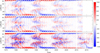 |
Fig. 1. Top: supersynoptic map of the observed radial component of the photospheric magnetic field at MWO. Middle and bottom: supersynoptic map derived from the PFSS solution of the photospheric radial field (nmax = 90). Middle panel: PFSS field derived from nonscaled MWO harmonic coefficients and bottom panel: PFSS field when MWO coefficients are scaled to SOLIS/VSM for 1974–2012 and SOLIS/VSM PFSS field for 2013–2017. |
The first panel of Fig. 1 shows the supersynoptic map (rotational longitudinal averages in time; also called the magnetic butterfly diagram) of the radial photospheric magnetic field derived from the original MWO observations. The radial component is derived from the line-of-sight by assuming that the field is radial in the photosphere (dividing BLOS by cosine of latitude). The middle and bottom panels show the scaled and nonscaled MWO supersynoptic maps derived from PFSS solution at the photosphere (r = Rs).
The top and middle panels of Fig. 1 look almost identical, which indicates that the PFSS model with nmax = 90 describes the longitudinal averages very well. One should note that in the longitudinally averaged PFSS field all terms with m ≠ 0 average to zero and therefore the longitudinally averaged PFSS field only depends on axial (m = 0) harmonics. The effect of scaling in the bottom panel of Fig. 1 is seen as a larger magnitude of the magnetic field at all latitudes, but the main patterns and the solar cycle evolution are more or less unchanged. The change from scaled MWO to SOLIS/VSM at the turn of 2012/2013 is not visible in the bottom panel of Fig. 1, which indicates that the MWO PFSS field scaled to SOLIS/VSM very much resembles the SOLIS/VSM PFSS field.
In the upper panel of Fig. 2 we first calculated the longitudinal means of the absolute values of both data sets for each rotation and then their ratios. The lower panel of Fig. 2 shows the ratio of the longitudinal means of the PFSS fields shown in the middle and bottom panels of Fig. 1 after first applying a threshold of 50 μT to the longitudinal means of the nonscaled data before calculating the ratio.
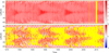 |
Fig. 2. Ratio between longitudinal means of scaled and nonscaled MWO photospheric PFSS radial fields (nmax = 90). Upper panel: ratio of longitudinal means of absolute field values. Lower panel: ratio of longitudinal means of signed field values. The longitudinal means of nonscaled PFSS field below 50 μT are excluded. Yellow color depicts data gaps due to missing observations or because of the intensity threshold. |
The upper panel of Fig. 2 depicts that the effective scaling factor from MWO to SOLIS/VSM is about three at mid-latitudes, but almost twice larger around the equator in the ascending to maximum phase of the solar cycle. Scaling factors around the poles are rather small (close to one) during solar minima, but are considerably larger during maxima. We note however that larger scaling factors are seen almost up to the pole during the previous solar minimum. The general pattern seems to be that scaling is smallest in the most unipolar field regions, especially for polar fields, and larger in regions where both polarities appear.
The lower panel of Fig. 2 shows a different configuration. Overall, the lower panel is relatively patchy while the upper panel depicts a smoother variation. Largest values in the lower panel are centered around the active regions, and show the equatorward drift (butterfly evolution) of the active regions, as well as a few individual poleward surges from active regions. There are only a few latitudes and rotations with (a small number of) negative ratios, which shows that the original and scaled means have, by a very large fraction, the same rotationally averaged polarities. Polar field scaling is quite similar in the upper and lower panels of Fig. 2, which is expected since polar fields are mainly unipolar and the rotational means of signed and absolute field values are closely similar.
Even though the harmonic scaling matrices do not vary in time, the effective scaling factors and their latitudinal variation have a significant solar cycle variability due to the varying relative contributions of the different harmonics over the solar cycle. We note that during solar maximum the effective latitudinal scaling factor of the absolute field (the ratios of the upper panel of Fig. 2) is somewhat similar to the latitudinal scaling factor of 4.5−2.5 sin2λ suggested by Ulrich (1992, see also later in Sect. 4).
We also note that the method of ratios used in Fig. 2 cannot be applied to original observations because, for example, of different noise levels in the different data sets. The observed magnetic field values include a significant contribution from noise, especially in the weak field areas. Noise levels between the different data sets vary significantly, but the harmonic coefficients of the PFSS model fields at least up to n = 90 are not significantly disturbed by noise (Paper II). This is one important benefit of the harmonic scaling method.
4. Scaling the coronal field
Figure 3 shows the supersynoptic maps of the coronal radial magnetic field using scaled and nonscaled MWO data and the PFSS model. The large-scale pattern and the solar cycle evolution of two panels are quite similar, but the magnitude of the coronal magnetic field is larger in the lower panel. The annual variation at low latitudes (due to the vantage point effect) seems to be reduced in the lower panel. This relates to the scaling of even axial terms, especially the axial quadrupole term  , which is affected by the vantage point effect and other problematic issues of high-latitude observations, like pole-filling (Virtanen & Mursula 2014, 2017). The
  scaling factor from MWO to SOLIS/VSM is 0.41 ± 0.49, which is significantly smaller than, for example, the dipole scaling factors (see Table A.7 in Paper II). This indicates that the vantage point effect and other problematic issues are more important for MWO than for SOLIS/VSM.
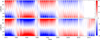 |
Fig. 3. Supersynoptic maps of the MWO PFSS radial field at the coronal source surface (nmax = 90, rss = 2.5Rs). Upper panel: magnetic field derived from nonscaled MWO harmonic coefficients, while lower panel: field when MWO photospheric harmonic coefficients are scaled to SOLIS/VSM. SOLIS/VSM coronal PFSS field for 2013–2017 is added in the lower panel. |
Figure 4 shows the ratio between the scaled and nonscaled coronal magnetic fields at the source surface (similarly to Fig. 2 for photospheric field). The upper panel of Fig. 4 depicts the ratio for the rotational means of the absolute field values and indicates that scaling is largest around the heliospheric current sheet (HCS; for more results on HCS, see Paper I). The PFSS magnetic field is weak in the HCS region and the large scaling factors at HCS in the upper panel of Fig. 4 reflect the above-mentioned alleviation of the vantage point effect in the SOLIS/VSM data as compared to MWO data. Outside the HCS region the scaling factor is typically between one and two and does not have a notable latitude variation. The average scaling factor in the upper panel of Fig. 4 is 1.35.
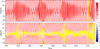 |
Fig. 4. Ratio between longitudinal means of scaled and nonscaled MWO coronal fields at Rss = 2.5Rs (nmax = 90). Upper panel: ratio of longitudinal means of absolute field values. Lower panel: ratio of longitudinal means of signed field values after removing values smaller than 1 μT. Yellow color depicts data gaps due to missing observations or because of the intensity threshold. |
The lower panel of Fig. 4 shows the ratio of the longitudinal means of the PFSS field in the upper and lower panels of Fig. 3 after first applying a threshold of 1 μT to the longitudinal means of the nonscaled data before calculating the ratio. As for photospheric fields, the polarities of the longitudinal means of nonscaled and scaled coronal fields mainly agree (most ratios are positive). The average scaling factor in the lower panel of Fig. 4 is 1.34, which is only slightly smaller than the ratio of absolute values. We also note that these ratios are close to the axial dipole scaling factor of 1.50 (see Appendix A.7 of paper II), the difference being largely due to the effect of even harmonics, such as axial quadrupole, which have scaling factors of below one.
Figure 5 shows the latitudinal variation of the effective scaling factors for the photospheric and coronal fields from MWO to SOLIS/VSM. One should note that the results in Fig. 5 are 11-year averages of effective latitudinal scaling factors, which have significant solar cycle variability, as depicted in Figs. 2 and 4. The observed MWO data was here re-sampled to the same 360*180 pixels longitude – sine-latitude grid as SOLIS/VSM in order to derive the ratios for the same latitudinal binning. In order to avoid very small values and singularities, absolute values smaller than 50 μT (1 μT) are excluded from the rotational averages of the photospheric (coronal) fields like in Figs. 2 and 4.
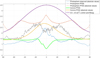 |
Fig. 5. Latitude variation of the effective scaling factors from MWO to SOLIS/VSM for photospheric and coronal fields. The blue curve is the ratio of averages of rotational means of absolute values observed by SOLIS/VSM and MWO over the overlapping period of two instruments in 2003–2013. The black (green) curve shows the ratio between scaled and nonscaled means of longitudinally averaged photospheric (coronal) PFSS magnetic fields. The red (yellow) curve shows the ratio between scaled and nonscaled means of longitudinally averaged absolute values of the photospheric (coronal) PFSS magnetic fields. The purple curve is the latitudinal scaling factor by Ulrich (1992) and Wang & Sheeley (1995). |
Figure 5 shows that when comparing observed absolute values of the photospheric field from SOLIS/VSM and MWO (blue curve in Fig. 5), the mean scaling factor at the equator is about 2.4 and decreases towards the poles. At mid-latitudes the scaling factor varies from 1 to 1.5 but at the poles it is about 1. However, we point out that the scaling factor derived from longitudinal means of absolute values of observed data might be misleading, for example because of the different resolutions of observations and noise levels in two data sets. These problems initially motivated the development of the harmonic scaling method.
The black curve in Fig. 5 shows that in case of signed values of the photospheric PFSS field the scaling factor is about 2.2 at the equator; it increases to about 2.9 at low latitudes and then decreases to about 1.5 at high latitudes. The black curve also shows much more bin-to-bin fluctuations than any other curve in Fig. 5. This is a consequence of signed values and the somewhat different topology and polarity structure of scaled and nonscaled MWO PFSS fields in the photosphere, which is also seen in the patchy structure of the lower panel of Fig. 2. The red curve in Fig. 5 shows that when using absolute values of the photospheric PFSS field, the mean effective harmonic scaling has its maximum of 3.6 at the equator, which is not very far from the factor of 4.5 given by Ulrich (1992) and Wang & Sheeley (1995). The scaling factor smoothly decreases from equator to about ±25°, where it has a local minimum of 2.85. It has a second local maximum of approximately 3.1 at about ±47° and a local minimum of 2.4 at ±79°, increasing again toward the pole. We note how closely this scaling factor and the one derived by Ulrich (1992) and Wang & Sheeley (1995) agree with one another over a considerable latitude range at mid- to high latitudes.
Coronal magnetic field is dominated only by a few lowest harmonics and therefore scaling mainly reflects the factors of those terms. The yellow curve in Fig. 5 shows that in case of absolute values the effective coronal scaling is about 2.9 at the equator and 1.4 at polar regions. We note that the latitude variation of this coronal curve is reminiscent of that of Ulrich (1992) and Wang & Sheeley (1995) for the photosphere, only some 50% lower. The effective scaling for the unsigned field has a rather narrow minimum of about 0.6 at the equator and a relatively constant value of about 1.4 beyond ±20° of latitude. The two coronal scaling factors of Fig. 5 and the two panels of Fig. 4 clearly show that the latitudinal variation is related to the proximity of the HCS.
5. Coronal flux density for different nmax and rss
Previous studies have shown that the coronal magnetic field and the heliospheric magnetic field can be described by using only a few of the lowest terms of the harmonic expansion (Wang 2014; Koskela et al. 2017). Figure 6 shows the mean unsigned coronal magnetic flux densities derived for nine different nmax values (nmax = 1–9) and for five different source surface radius values (rss = 1.5RS–3.5RS) using the entire data set. We note that the values of the different data sets in Fig. 6 cannot be directly compared since they represent different time intervals, as shown in Table 1.
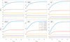 |
Fig. 6. Dependence of mean coronal magnetic flux density ⟨|Br(r)|⟩ on nmax from 1 to 9 and on source surface radius rss from 1.5RS to 3.5RS. For comparison, all values have been scaled to 2.5Rs by multiplying with (2.5Rs/rss)2. |
The general pattern in Fig. 6 is that rss and ⟨|Br(r)|⟩ are roughly inversely proportional. The larger the source surface distance is, the more flux is enclosed within it, leaving less flux to be open. On the other hand, ⟨|Br(r)|⟩ naturally increases with nmax, as the higher multipoles give additional contributions to the absolute flux density. However, the increase of the flux with nmax is highly nonlinear, and is saturated already at relatively low nmax. This is because the higher multipoles decrease increasingly quickly with radial distance (see Eqs. (1) and (2)). Accordingly, their contribution to the coronal field is small, although it can be significant at the photosphere.
As Fig. 6 shows, the effect of increasing nmax becomes smaller with increasing rss. When rss ≥ 2.0RS, all data sets depict little change beyond nmax = 2 and reach the final maximum already at nmax = 4. Thus, nmax = 4 is sufficiently large to describe the mean PFSS coronal unsigned flux density for all data sets when rss ≥ 2.0RS. For rss = 1.5RS, the pattern is different and some increase in ⟨|Br(r)|⟩ is seen until nmax = 9. However, the value of rss = 1.5RS is too small, as it leads to excessively large coronal hole areas (Linker et al. 2017) and unrealistic HMF sector structures (Koskela et al. 2017).
For the largest source surface radius of 3.5RS included in Fig. 6, the coronal magnetic field is close to a dipole (nmax = 1), and adding the higher multipoles up to nmax = 9 would increase ⟨|Br(r)|⟩ only by 1–11%, depending on the data set used. Correspondingly, for rss values of 3.0RS, 2.5RS, 2.0RS and 1.5RS the harmonics from n = 2 to n = 9 would add up to about 2–15%, 3–23%, 8–43% and 27–112% with respect to the dipole term. Wang et al. (2000) suggested that the heliospheric unsigned flux density mainly follows the absolute value of solar  dipole strength. This is in agreement with our results, which show that in the case of a sufficiently large value of rss only the lowest harmonic defines the coronal (and heliospheric) magnetic field. We note that the contribution of higher harmonics varies over the solar cycle. During most of the solar cycle the field is almost dipolar, but becomes more complicated during the ascending to maximum phase of solar cycle (see Fig. 3).
Figure 7 shows that the mean photospheric and coronal magnetic flux densities depends on nmax. We use SOLIS/VSM data here since it covers more than one solar cycle and has a high spatial resolution, thus allowing us to study the dependence of nmax. The upper panel of Fig. 7 shows that the photospheric ⟨|Br(r)|⟩ systematically and significantly increases with nmax. The relative increase of ⟨|Br(r)|⟩ when nmax grows from 1 to 90 is about one order of magnitude during solar maximum times in 2014–2015. During solar minimum times this increase is smaller because the high harmonics decrease with lower solar activity but the dipole term increases. The ⟨|Br(r)|⟩ for the observed data at a resolution of 360*180 very closely resembles ⟨|Br(r)|⟩ from PFSS with nmax = 90 and the ratio between their means is 1.0. The observed data at 1800*900 pixels shows the largest ⟨|Br(r)|⟩ values, as expected. This directly relates to the fact that opposite polarities cancel each other when averaging to lower resolution. The ratio of observed mean ⟨|Br(r)|⟩ between resolutions of 1800*900 and 360*180 is 1.4, which is the same as the ratio of the observed ⟨|Br(r)|⟩ between a resolution of 1800*900 pixels and PFSS with nmax = 90.
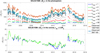 |
Fig. 7. Dependence of mean photospheric and coronal magnetic flux density ⟨|Br(r)|⟩ on nmax. Upper panel: rotational values of ⟨|Br(r)|⟩ in the photosphere (r = Rs) with nmax = 1, 2, 5, 10, 20, 50, 90 and the observed values from synoptic maps of 1800*900 and 360*180 pixels, respectively. Lower panel: ⟨|Br(r)|⟩ in the coronal source surface (rss = 2.5RS) using the same values of nmax as in the upper panel. |
The lower panel of Fig. 7 shows that at the coronal source surface even the dipole term (nmax = 1) alone defines the ⟨|Br(r)|⟩ fairly well over most of the solar cycle. The largest difference between nmax = 1 and the higher harmonics (temporally more than 100%) is seen in the ascending phase of solar cycle 24 in 2012. The ⟨|Br(r)|⟩ does not significantly increase beyond nmax = 2 and beyond nmax = 5; adding higher multipoles has no effect (curves for nmax = 5−90 are exactly on top of each other). The smaller difference between the different nmax values in the lower panel of Fig. 7 is a direct consequence of the fast radial decay of high harmonics. Moreover, as we can infer from Fig. 6, the chosen source surface radius distance rss = 2.5Rs is sufficiently large to reduce the effect of higher harmonics to ⟨|Br(r)|⟩.
6. Nonscaled coronal unsigned magnetic flux density
Figure 8 shows the rotational values of nonscaled coronal unsigned magnetic flux density ⟨|Br(r)|⟩ for the six data sets using nmax = 9. The basic patterns are in agreement with Fig. 6 and Paper II. For rss = 3.5Rs and rss = 2.5Rs the different data sets show a relatively similar cyclic behavior. The only significant difference between results for rss = 3.5Rs and rss = 2.5Rs is that values for the latter are about 2.7 times larger, which closely corresponds to the r−3 radial decrease of the dipole term ((3.5/2.5)3 ≈ 2.7). The minimum ⟨|Br(r)|⟩ is reached during the ascending or maximum phase of the solar cycles in 1979, 1990, 1999–2000 and 2012–2013. The different data sets show the cycle minima at fairly similar times, separated by approximately one year. For rss = 3.5Rs and rss = 2.5Rs the cycle maxima of ⟨|Br(r)|⟩ are found in the early declining phase of the solar cycle in 1981–1982, 1991, 2002–2003 and 2014–2015.
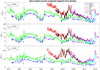 |
Fig. 8. Original nonscaled coronal magnetic flux densities derived from six independent data sets of source surface radii rss of 2.5RS and 1.5RS. Upper, middle, and lower panels: results for rss = 3.5Rs, rss = 2.5Rs, and rss = 1.5Rs, respectively. |
For rss = 1.5Rs the magnetic flux density ⟨|Br(r)|⟩ fluctuates over the solar cycle in a different manner compared to that for rss = 3.5Rs and rss = 2.5Rs. This relates to the larger relative contribution of higher-order terms, which tend to have a larger (and somewhat different) solar cycle variation than the lowest terms. For rss = 1.5Rs the minima of ⟨|Br(r)|⟩ are typically at different times compared to those for rss = 2.5Rs and rss = 3.5Rs, and they differ more between the different data sets. The flux levels in the ascending and maximum phase rise relative to rss = 3.5Rs or rss = 2.5Rs due to new flux increasing the higher harmonic terms. This shifts the ⟨|Br(r)|⟩ minima mostly to the late declining to minimum phase of the solar cycle in 1975–1976, 1995–1997, and 2009. On the other hand, ⟨|Br(r)|⟩ cycle maxima for rss = 1.5Rs are not significantly different from those for rss = 3.5Rs and rss = 2.5Rs. The maxima of solar cycles 21, 22, and 24 for rss = 1.5Rs are found in 1981–1982, 1991, and 2014–2015, similarly to rss = 3.5Rs and rss = 2.5Rs. In the late 1990s and late 2005, ⟨|Br(r)|⟩ is relatively much larger for rss = 1.5Rs than for rss = 3.5Rs and rss = 2.5Rs. Still, most data sets depict the maximum of cycle 23 to be in 2002–2003 also for rss = 1.5Rs. Only MDI shows the corresponding maximum already in 1999.
For rss = 3.5Rs, rss = 2.5Rs, and rss = 1.5Rs the mean ⟨|Br(r)|⟩ (over the common time interval) is largest in SOLIS/VSM and KP, slightly smaller in MDI and HMI, significantly smaller in MWO, and smallest in WSO. While the flux density ⟨|Br(r)|⟩ and its solar cycle evolution depend on the used rss value, all data sets that cover several solar cycles (mainly WSO and MWO) depict a gradual decrease of the average ⟨|Br(r)|⟩ minimum values decreasing from around 1990 and having maximum values in the early 1980s. Cycle minimum values of ⟨|Br(r)|⟩ for rss = 3.5Rs and rss = 2.5Rs in WSO and MWO have decreased by about 60%, from their minimum in cycle 22 of 1990 to their minimum in cycle 24 of 2012. For rss = 1.5Rs a similar decrease of ⟨|Br(r)|⟩ minimum by about 50% is observed from the late 1980s to 2009. The maximum values of ⟨|Br(r)|⟩ for both WSO and MWO decreased by about 30% from the early 1980s to early 2000s for all rss values.
7. Scaled coronal unsigned magnetic flux density
With the harmonic scaling method described above and in Paper II, we are able to scale the harmonic coefficients of the six data sets to each other. This allows for ⟨|Br(r)|⟩ to be scaled to the same level for all six data sets. We use all six data sets as reference stations to which all other data sets are scaled. This allows for a detailed comparison to be made of the long-term time evolution of ⟨|Br(r)|⟩ according to each station. Since there is no time overlap between KP and SOLIS/VSM, nor between KP and HMI, those pairings cannot be calculated.
Figure 9 shows the unsigned coronal magnetic flux densities (nmax = 9) using each of the six stations as a reference to which all other stations that have a sufficient overlapping period in observations have been scaled. Scaling has been made using two source surface distances, rss = 2.5Rs (left panel) and rss = 1.5Rs (right panel). The case of rss = 3.5Rs is left out because it closely resembles the case of rss = 2.5Rs as already seen in Fig. 8. Nonscaled values of ⟨|Br(r)|⟩ in each panel of Fig. 9 duplicate the corresponding curve of Fig. 8. Therefore, for the period of the nonscaled data, the time evolution and the location of ⟨|Br(r)|⟩ minima and maxima follow the results discussed in Fig. 8.
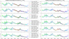 |
Fig. 9. Scaled coronal magnetic flux densities derived from six data sets for nmax = 9 using source surface radii of 2.5RS (left) and 1.5RS (right). In the upper row all other data sets have been scaled to WSO data. In the lower rows, MWO, KP, SOLIS/VSM MDI and HMI are use as the reference station to which all the other data sets are scaled. |
Figure 9 shows that scaling works very well in general and that the scaled flux densities are typically quite close to the reference station and each other in each case. Moreover, the time evolutions of unsigned fluxes for the different reference stations for rss = 2.5Rs greatly resemble each other, but the absolute levels of ⟨|Br(r)|⟩ vary.
Interestingly, the fluxes for rss = 1.5Rs (right panels of Fig. 9) show larger mutual differences in their time evolution than fluxes for rss = 2.5Rs. We find a relatively similar time evolution of ⟨|Br(r)|⟩ when WSO or MWO are used as a reference station to scale the other data sets. However, when KP, SOLIS/VSM or MDI are used as reference stations, the location of the minimum ⟨|Br(r)|⟩ in 1988–1989 in WSO and MWO is shifted to 1987 and the minimum of the 1990s is shifted from 1999 to 1997. This was already seen for the 1990s minimum in the nonscaled fluxes in Fig. 8, and Fig. 9 shows a similar shift of minimum for scaled fluxes. Similarly, the 2009 minimum is independent of the reference station used, both for the scaled and nonscaled fluxes for rss = 1.5Rs.
8. Magnetic flux density between photosphere and source surface
In order to study the effect of scaling inside the corona, we show in Fig. 10 the scaled unsigned magnetic flux densities at four altitudes from the photosphere to the source surface 2.5RS. We use here SOLIS/VSM as the reference data set to which all other data sets are scaled (as in the fourth row of Fig. 9).
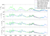 |
Fig. 10. Scaled magnetic flux densities at four altitudes from photosphere to the source surface(1RS, 1.5RS, 2.0RS and 2.5RS) for four data sets scaled to SOLIS (nmax = 90 for others, 9 for WSO). Upper panel: dark-green curve shows the observed (not PFSS modeled) unsigned magnetic flux density of SOLIS/VSM (360*180 resolution). Second and third panels: ⟨|Br(r)|⟩ at r = 1.5Rs and r = 2.0Rs and fourth panel: at the source surface of r = 2.5Rs. |
The upper panel of Fig. 10 shows that the nonscaled PFSS SOLIS/VSM, the HMI and MDI PFSS scaled to SOLIS/VSM (nmax = 90), and the observed SOLIS/VSM (360*180) flux densities all agree very well. This verifies that the potential field with nmax = 90 describes the photospheric flux density quite reliably. On the other hand, WSO depicts smaller field values in the photosphere because of its low resolution and smaller nmax. However, we note that WSO agrees with the level of the other data sets already at r = 1.5Rs.
All data sets agree on the fact that the photospheric magnetic flux density (see upper panel of Fig. 10) always starts to increase right after the sunspot minimum. However, the coronal field at r = rss = 2.5Rs starts to increase, as already discussed above, only around the cycle maximum. The coronal field evolution is similar also in WSO, even though only harmonics up to nmax = 9 are used. This similarity is related to the fast radial decrease of the high-order harmonic terms. Low harmonics dominate around solar minima but start to decrease thereafter when new flux appears in the photosphere. However, the new flux does not immediately contribute to the source surface field; this only happens around sunspot maximum when low harmonics have almost disappeared and high harmonics dominate.
9. Discussion
Here, we used the harmonic scaling method presented in Paper II to scale the observations of the photospheric magnetic field between different data sets. One motivation of this work is to correct WSO and MWO, the two longest time series of photospheric magnetic field observations, which are known to underestimate the photospheric magnetic flux due for example to line saturation (Svalgaard et al. 1978; Ulrich 1992; Wang & Sheeley 1995). The more recent higher-resolution instruments tend to suffer less from saturation, but their time span is rather short.
The PFSS model with nmax = 90 gives a fairly reliable approximation of the observed MWO photospheric magnetic field, which can then be scaled to the SOLIS/VSM. The scaled MWO PFSS field closely resembles the observed photospheric SOLIS/VSM field as well as the coronal SOLIS/VSM field at the source surface. The most significant difference between nonscaled and scaled MWO PFSS data at 2.5Rs is the reduced annual oscillation of HCS in the scaled data. This is a direct consequence of the smaller  quadrupole term in scaled data due to the small scaling factor.
The effective latitudinal scaling factors from MWO to SOLIS/VSM (see Fig. 5) depend on the averaging method. Scaling factors are typically larger when comparing latitudinal averages of absolute field values. This is mainly a consequence of differences in the detailed spatial distribution of field values in original MWO and SOLIS/VSM observations, as well as in the scaled and nonscaled MWO data. Moreover, the noise is different in the two instruments, which causes differences between the mean field values. We also point out that the overlapping time interval between MWO and SOLIS/VSM observations is only about 10 years. This is sufficient to cover changes over the solar cycle, but not possible long-term changes.
The effective latitudinal scaling factor in the photosphere is typically largest at low latitudes or the equator and decreases towards the poles. Depending on the method of derivation, the equatorial scaling factor is 2.0–3.6, the low-latitude (active region) scaling factor is 1.5–2.9, and the high-latitude scaling factor is 1–2.5. We note that the reliability of the equatorial scaling factor is somewhat questionable since equatorial magnetic fields are very weak in general, especially in the case of signed rotational means. Latitudinal effective scaling factors are in agreement with the results of Paper II, where we found that when scaling low-resolution data to high-resolution data, scaling factors increase with harmonic order. In the case of scaling MWO to SOLIS/VSM, the scaling factor for axial dipole is 1.50, but the mean scaling factor up to n = 90 is 3.86. Because low-latitude active regions mainly reflect higher harmonics and polar fields reflect the axial dipole, effective latitudinal scaling is larger at low latitudes. For absolute field values, the coronal scaling factor has a maximum of about 2.9 at the equator, but for signed values this factor has a minimum of about 0.6. This is a consequence of the vicinity of the HCS at low latitudes. The high-latitude scaling factor is about 1.4 in both cases, which reflects the unipolar high-latitude fields.
Coronal source surface magnetic field can be reliably modeled using only the lowest harmonics up to nmax = 5. Figure 6 shows that adding higher harmonics changes the amount of flux significantly only for rss = 1.5Rs but for rss ≥ 2.5Rs the flux does not change beyond nmax = 3. Figure 7 confirms that in the case of SOLIS/VSM PFSS the coronal field with nmax = 5 gives exactly the same unsigned magnetic flux density ⟨|Br(r)|⟩ as with nmax = 90 (or any value between them). On the other hand, in the photosphere ⟨|Br(r)|⟩ increases with nmax, and nmax = 90 agrees very well with the observed SOLIS/VSM ⟨|Br(r)|⟩ derived from 360*180 pixel synoptic maps. For the 1800*900-pixel high-resolution maps the ⟨|Br(r)|⟩ is systematically slightly larger. Figure 8 shows that the different nonscaled photospheric data sets depict different absolute levels and even different solar cycle evolutions for the coronal ⟨|Br(r)|⟩. While the six data sets agree with each other when using rss = 3.5Rs or rss = 2.5Rs, for rss = 1.5Rs the high-resolution data sets (KP, MDI, SOLIS/VSM and HMI) depict different solar cycle evolution.
Different data sets show quite similar results for the unsigned coronal magnetic flux density ⟨|Br(r)|⟩ when harmonic scaling is applied. When the source surface radius is 3.5Rs or 2.5Rs, using different instruments as a reference data set to scale the others leads to a relatively similar solar cycle evolution of ⟨|Br(r)|⟩ for all data sets. The minima of ⟨|Br(r)|⟩ are around 1979, 1990, 1999–2000, and 2012–2013, and maximum in 1981–1982, 1991, 2002–2003 (1999 in MDI), and 2014–2015. However, for rss = 1.5Rs, the different reference data sets lead to a rather different solar cycle evolution. When KP, MDI, SOLIS/VSM or HMI is used as a reference station, minima are located in the later declining to minimum phase of the solar cycle in 1975–1976, 1995–1997, and 2009. This is because the scaling of WSO and MWO observations to higher-resolution and less-saturated data sets increases the relative fraction of higher harmonics. The contribution of higher harmonics, which have a relatively small fraction in nonscaled WSO and MWO data, increases when lowering the source surface radius. This is particularly important during the ascending phase of the cycle, when low multipoles, especially the axial dipole, weaken and the higher multipole terms strengthen rapidly.
Harmonic scaling method can be applied to any pair of data sets with a sufficiently long overlapping period, despite resolution differences between data sets. However, the maximum resolution and the highest possible PFSS harmonic nmax for the scaled field is determined by the resolution (and the corresponding nmax) of the original data. Figure 10 shows that this limitation is important in the photosphere, where ⟨|Br(r)|⟩ for WSO scaled to SOLIS/VSM remains significantly smaller than for the other data sets with higher resolution. However, already at r = 1.5Rs (rss = 2.5Rs) the scaled WSO field agrees very well with other scaled data sets.
The results of this paper show that the distance of the source surface radius has a significant impact on the solar cycle evolution and the absolute level of ⟨|Br(r)|⟩. The question of a correct source surface radius is complicated. In this paper we have shown that the source surface radius significantly affects the coronal magnetic flux derived from the PFSS model and even the time evolution of coronal flux density. The topology of the field (sector structure), the unsigned magnetic flux, and coronal hole areas all depend on the data set, the pole-filling method, and the source surface radius. Source surface is typically defined as a sphere with a constant radius, typically between 1.5 and 3.5 solar radii. However, it has been shown that the shape may not be a sphere and the radius may vary over the solar cycle (Lee et al. 2011; Arden et al. 2014; Koskela et al. 2017). It is in principle possible to determine the true source surface radius (and its topological structure) from coronagraph or solar eclipse images (like Fig. 1 in Habbal et al. 2010), but the lack of low-coronal coronagraphs and the rareness of eclipses makes this practically impossible for long-term studies. Recent studies also indicate that, at least occasionally, it is impossible to define the source surface radius which would give a correct unsigned magnetic flux and a realistic coronal hole area within the PFSS model assumptions (Linker et al. 2017). This raises the question of whether all solar wind and magnetic flux indeed originate from coronal holes, or whether another mechanism exists which is not included in the PFSS model. The question of solar wind sources and the definition of the best source surface radius will be discussed in a future article.
10. Conclusions
Synoptic maps of the photospheric magnetic field are widely used in solar research, especially in the modeling of the solar corona and the solar wind, as well as when estimating the effects on space weather and space climate. One major issue for long-term studies has been that the observed photospheric magnetic flux depends on the instrument and data processing used. We have recently developed a method to scale the observations in terms of harmonic expansion (Virtanen & Mursula 2017). Harmonic scaling can be applied to scale any pair of synoptic data regardless of their resolution, which facilitates the comparison and allows for a long-term uniform data set to be constructed.
In this paper we used the harmonic scaling method to calculate effective latitudinal scaling factors which vary over the solar cycle. Effective scaling factors are typically largest at low latitudes during the ascending phase of the solar cycle and are smallest in unipolar polar fields during solar minimum times. We find that the coronal magnetic flux density can be correctly scaled using only the lowest harmonics up to about nmax = 5 in the PFSS model. When using original nonscaled observations the unsigned magnetic flux density depends on the data set at any altitude between photosphere and coronal source surface. However, harmonic scaling sets the observations to the same intensity level at all coronal altitudes from photosphere to the source surface.
The unsigned magnetic flux derived from the different scaled data sets has a similar solar cycle variability for all data sets for rss = 2.5Rs and rss = 3.5Rs. However, the location of solar cycle minima and maxima depends on the reference data set for rss = 1.5Rs. This is a consequence of the varying contribution of the different harmonics during the solar cycle. Scaling changes the relative fraction of harmonics and a low source surface radius emphasizes the relative contribution of higher harmonics. Scaled magnetic flux densities depict a systematic long-term decrease of ⟨|Br(r)|⟩. Cycle minimum values of ⟨|Br(r)|⟩ (for rss = 3.5Rs and rss = 2.5Rs) in WSO and MWO have decreased from cycle 22 minimum to cycle 24 minimum by about 60%.
The most reliable data set and the optimum value of the coronal source surface radius to be used in the PFSS model remain to be fully determined and will be further investigated in subsequent studies.
Acknowledgments
We acknowledge the financial support by the Academy of Finland to the ReSoLVE Centre of Excellence (project no. 307411). Wilcox Solar Observatory data used in this study were obtained via the web site http://wso.stanford.edu courtesy of J.T. Hoeksema. This study includes data from the synoptic program at the 150-Foot Solar Tower of the Mt. Wilson Observatory, which is acknowledged. NSO/Kitt Peak magnetic data used here are produced cooperatively by NSF/NOAO, NASA/GSFC and NOAA/SEL. Data were acquired by SOLIS instruments operated by NISP/NSO/AURA/NSF. SOHO/MDI is a project of international cooperation between ESA and NASA. HMI data are courtesy of the Joint Science Operations Center (JSOC) Science Data Processing team at Stanford University. Authors are members of international team on Reconstructing Solar and Heliospheric Magnetic Field Evolution Over the Past Century supported by the International Space Science Institute (ISSI), Bern, Switzerland. Data used in this study was obtained from the following web sites: WSO: http://wso.stanford.edu, MWO: ftp://howard.astro.ucla.edu/pub/obs/synoptic_charts/fits/, Kitt Peak: ftp://solis.nso.edu/kpvt/synoptic/mag/, MDI: http://soi.stanford.edu/magnetic/synoptic/carrot/M_Corr, HMI: http://jsoc.stanford.edu/data/hmi/synoptic, SOLIS/VSM: http://solis.nso.edu/0/vsm/vsm_maps.php .
References
- Altschuler, M. D., & Newkirk, G. 1969, Sol. Phys., 9, 131 [Google Scholar]
- Arden, W. M., Norton, A. A., & Sun, X. 2014, J. Geophys. Res. (Space Phys.), 119, 1476 [NASA ADS] [CrossRef] [Google Scholar]
- Arge, C. N., & Pizzo, V. J. 2000, J. Geophys. Res., 105, 10465 [NASA ADS] [CrossRef] [Google Scholar]
- Arge, C. N., Henney, C. J., Koller, J., et al. 2010, Twelfth Int. Sol. Wind Conf., 1216, 343 [NASA ADS] [Google Scholar]
- Asvestari, E., & Usoskin, I. G. 2016, J. Space Weather Space Clim., 6, A15 [CrossRef] [EDP Sciences] [Google Scholar]
- Erdös, G., & Balogh, A. 2014, ApJ, 781, 50 [NASA ADS] [CrossRef] [Google Scholar]
- Habbal, S. R., Druckmüller, M., Morgan, H., et al. 2010, ApJ, 719, 1362 [NASA ADS] [CrossRef] [Google Scholar]
- Henney, C. J., Keller, C. U., & Harvey, J. W. 2006, in ASP Conf. Ser., eds. R. Casini, & B. W. Lites, 358, 92 [NASA ADS] [Google Scholar]
- Hoeksema, J. T., Wilcox, J. M., & Scherrer, P. H. 1983, J. Geophys. Res., 88, 9910 [NASA ADS] [CrossRef] [Google Scholar]
- Jiang, J., Cameron, R. H., Schmitt, D., & Schüssler, M. 2011, A&A, 528, A83 [NASA ADS] [CrossRef] [EDP Sciences] [Google Scholar]
- Keller, C. U., & Solis Team 2001, in Advanced Solar Polarimetry – Theory, Observation, and Instrumentation, ed. M. Sigwarth, ASP Conf. Ser., 236, 16 [NASA ADS] [Google Scholar]
- Koskela, J. S., Virtanen, I. I., & Mursula, K. 2017, ApJ, 835, 63 [NASA ADS] [CrossRef] [Google Scholar]
- Lee, C. O., Luhmann, J. G., Zhao, X. P., et al. 2009, Sol. Phys., 256, 345 [NASA ADS] [CrossRef] [Google Scholar]
- Lee, C. O., Luhmann, J. G., Hoeksema, J. T., et al. 2011, Sol. Phys., 269, 367 [Google Scholar]
- Linker, J. A., Caplan, R. M., Downs, C., et al. 2017, ApJ, 848, 70 [NASA ADS] [CrossRef] [Google Scholar]
- Lockwood, M., Owens, M., & Rouillard, A. P. 2009, J. Geophys. Res., 114, 11104 [CrossRef] [Google Scholar]
- Malanushenko, A., Schrijver, C. J., DeRosa, M. L., & Wheatland, M. S. 2014, ApJ, 783, 102 [NASA ADS] [CrossRef] [Google Scholar]
- Mays, M. L., Taktakishvili, A., Pulkkinen, A., et al. 2015, Sol. Phys., 290, 1775 [CrossRef] [Google Scholar]
- Parker, E. N. 1965, Planet. Space Sci., 13, 9 [Google Scholar]
- Riley, P., Linker, J. A., Mikić, Z., et al. 2006, ApJ, 653, 1510 [Google Scholar]
- Schatten, K. H., Wilcox, J. M., & Ness, N. F. 1969, Sol. Phys., 6, 442 [Google Scholar]
- Stevens, M. L., Linker, J. A., Riley, P., & Hughes, W. J. 2012, J. Atmos. Sol. Terr. Phys., 83, 22 [Google Scholar]
- Svalgaard, L., Duvall, Jr., T. L., & Scherrer, P. H. 1978, Sol. Phys., 58, 225 [Google Scholar]
- Tlatov, A., Tavastsherna, K., & Vasil’eva, V. 2014, Sol. Phys., 289, 1349 [NASA ADS] [CrossRef] [Google Scholar]
- Ulrich, R. K. 1992, in Cool Stars, Stellar Systems, and the Sun, eds. M. S. Giampapa, & J. A. Bookbinder, ASP Conf. Ser., 26, 265 [NASA ADS] [Google Scholar]
- Virtanen, I. I., & Mursula, K. 2014, ApJ, 781, 99 [Google Scholar]
- Virtanen, I., & Mursula, K. 2016, A&A, 591, A78 [NASA ADS] [CrossRef] [EDP Sciences] [Google Scholar]
- Virtanen, I., & Mursula, K. 2017, A&A, 604, A7 [NASA ADS] [CrossRef] [EDP Sciences] [Google Scholar]
- Wang, Y.-M. 2014, Space Sci. Rev., 186, 387 [NASA ADS] [CrossRef] [Google Scholar]
- Wang, Y.-M., & Sheeley, Jr., N. R. 1995, ApJ, 447, L143 [NASA ADS] [Google Scholar]
- Wang, Y.-M., Lean, J., & Sheeley, Jr., N. R. 2000, Geophys. Res. Lett., 27, 505 [Google Scholar]
- Wiegelmann, T., Petrie, G. J. D., & Riley, P. 2015, Space Sci. Rev. [Google Scholar]
- Zhao, X., & Hoeksema, J. T. 1995, Adv. Space Res., 16 [Google Scholar]
All Tables
All Figures
|
Fig. 1. Top: supersynoptic map of the observed radial component of the photospheric magnetic field at MWO. Middle and bottom: supersynoptic map derived from the PFSS solution of the photospheric radial field (nmax = 90). Middle panel: PFSS field derived from nonscaled MWO harmonic coefficients and bottom panel: PFSS field when MWO coefficients are scaled to SOLIS/VSM for 1974–2012 and SOLIS/VSM PFSS field for 2013–2017. |
| In the text | |
|
Fig. 2. Ratio between longitudinal means of scaled and nonscaled MWO photospheric PFSS radial fields (nmax = 90). Upper panel: ratio of longitudinal means of absolute field values. Lower panel: ratio of longitudinal means of signed field values. The longitudinal means of nonscaled PFSS field below 50 μT are excluded. Yellow color depicts data gaps due to missing observations or because of the intensity threshold. |
| In the text | |
|
Fig. 3. Supersynoptic maps of the MWO PFSS radial field at the coronal source surface (nmax = 90, rss = 2.5Rs). Upper panel: magnetic field derived from nonscaled MWO harmonic coefficients, while lower panel: field when MWO photospheric harmonic coefficients are scaled to SOLIS/VSM. SOLIS/VSM coronal PFSS field for 2013–2017 is added in the lower panel. |
| In the text | |
|
Fig. 4. Ratio between longitudinal means of scaled and nonscaled MWO coronal fields at Rss = 2.5Rs (nmax = 90). Upper panel: ratio of longitudinal means of absolute field values. Lower panel: ratio of longitudinal means of signed field values after removing values smaller than 1 μT. Yellow color depicts data gaps due to missing observations or because of the intensity threshold. |
| In the text | |
|
Fig. 5. Latitude variation of the effective scaling factors from MWO to SOLIS/VSM for photospheric and coronal fields. The blue curve is the ratio of averages of rotational means of absolute values observed by SOLIS/VSM and MWO over the overlapping period of two instruments in 2003–2013. The black (green) curve shows the ratio between scaled and nonscaled means of longitudinally averaged photospheric (coronal) PFSS magnetic fields. The red (yellow) curve shows the ratio between scaled and nonscaled means of longitudinally averaged absolute values of the photospheric (coronal) PFSS magnetic fields. The purple curve is the latitudinal scaling factor by Ulrich (1992) and Wang & Sheeley (1995). |
| In the text | |
|
Fig. 6. Dependence of mean coronal magnetic flux density ⟨|Br(r)|⟩ on nmax from 1 to 9 and on source surface radius rss from 1.5RS to 3.5RS. For comparison, all values have been scaled to 2.5Rs by multiplying with (2.5Rs/rss)2. |
| In the text | |
|
Fig. 7. Dependence of mean photospheric and coronal magnetic flux density ⟨|Br(r)|⟩ on nmax. Upper panel: rotational values of ⟨|Br(r)|⟩ in the photosphere (r = Rs) with nmax = 1, 2, 5, 10, 20, 50, 90 and the observed values from synoptic maps of 1800*900 and 360*180 pixels, respectively. Lower panel: ⟨|Br(r)|⟩ in the coronal source surface (rss = 2.5RS) using the same values of nmax as in the upper panel. |
| In the text | |
|
Fig. 8. Original nonscaled coronal magnetic flux densities derived from six independent data sets of source surface radii rss of 2.5RS and 1.5RS. Upper, middle, and lower panels: results for rss = 3.5Rs, rss = 2.5Rs, and rss = 1.5Rs, respectively. |
| In the text | |
|
Fig. 9. Scaled coronal magnetic flux densities derived from six data sets for nmax = 9 using source surface radii of 2.5RS (left) and 1.5RS (right). In the upper row all other data sets have been scaled to WSO data. In the lower rows, MWO, KP, SOLIS/VSM MDI and HMI are use as the reference station to which all the other data sets are scaled. |
| In the text | |
|
Fig. 10. Scaled magnetic flux densities at four altitudes from photosphere to the source surface(1RS, 1.5RS, 2.0RS and 2.5RS) for four data sets scaled to SOLIS (nmax = 90 for others, 9 for WSO). Upper panel: dark-green curve shows the observed (not PFSS modeled) unsigned magnetic flux density of SOLIS/VSM (360*180 resolution). Second and third panels: ⟨|Br(r)|⟩ at r = 1.5Rs and r = 2.0Rs and fourth panel: at the source surface of r = 2.5Rs. |
| In the text | |
Current usage metrics show cumulative count of Article Views (full-text article views including HTML views, PDF and ePub downloads, according to the available data) and Abstracts Views on Vision4Press platform.
Data correspond to usage on the plateform after 2015. The current usage metrics is available 48-96 hours after online publication and is updated daily on week days.
Initial download of the metrics may take a while.