| Issue |
A&A
Volume 625, May 2019
|
|
|---|---|---|
| Article Number | A3 | |
| Number of page(s) | 7 | |
| Section | The Sun | |
| DOI | https://doi.org/10.1051/0004-6361/201935188 | |
| Published online | 29 April 2019 | |
Pulse-beam heating of deep atmospheric layers, their oscillations and shocks modulating the flare reconnection
1
University of South Bohemia, Faculty of Science, Institute of Physics, Branišovská 1760, 370 05 České Budějovice, Czech Republic
e-mail: This email address is being protected from spambots. You need JavaScript enabled to view it.
2
Astronomical Institute of the Czech Academy of Sciences, Fričova 258, 251 65 Ondřejov, Czech Republic
Received:
1
February
2019
Accepted:
20
February
2019
Abstract
Aims. We study the processes occurring after a sudden heating of deep atmospheric layers at the flare arcade footpoints, which is assumed to be caused by particle beams.
Methods. For the numerical simulations we adopt a 2D magnetohydrodynamic (MHD) model, in which we solve a full set of the time-dependent MHD equations by means of the FLASH code, using the adaptive mesh refinement (AMR) method.
Results. In the initial state we consider a model of the solar atmosphere with densities according to the VAL-C model and the magnetic field arcade having the X-point structure above, where the magnetic reconnection is assumed. We found that the sudden pulse-beam heating of deep atmospheric layers at the flare arcade footpoints generates two magnetohydrodynamic shocks, one propagating upwards and the second propagating downwards in the solar atmosphere. The downward-moving shock is reflected at deep and dense atmospheric layers and triggers oscillations of these layers. The period of these oscillations in our case is about 174 s. These oscillations generate the upward-moving magnetohydrodynamic waves that can influence the flare magnetic reconnection in a quasi-periodic way. These processes require a sudden heating in very localized regions in dense atmospheric layers; therefore, they can be also associated with seismic waves.
Key words: Sun: flares / Sun: oscillations / methods: numerical / magnetohydrodynamics (MHD)
© ESO 2019
1. Introduction
In solar flares oscillations are quite typical. They are observed in a broad range of electromagnetic emission from radio, soft X-ray, hard X-ray, ultraviolet up to gamma rays (see e.g., Roberts et al. 1984; Fárník et al. 2003; Wang et al. 2005; Nakariakov et al. 2006, 2010). These oscillations have periods in the range from sub-seconds to tens of minutes (Mészárosová et al. 2006; Tan 2008; Karlický et al. 2010; Kupriyanova et al. 2010; Huang et al. 2014; Nisticò et al. 2014). Many models of these oscillations have been proposed; very important among them is the simulation presented by Takasao & Shibata (2016), where the authors, including essential physics, have found the spontaneously generated above-the-loop-top oscillation (for further simulations, see also the papers by Jelínek & Murawski 2013; Guo et al. 2016; Jelínek et al. 2017, and for a review, see e.g. the papers by Pascoe 2014; Nakariakov et al. 2016; McLaughlin et al. 2018).
During the impulsive phase of solar flares it is commonly accepted that particle beams, which are accelerated by the magnetic reconnection in the low corona, propagate downwards along the legs of the flare arcade and bombard dense atmospheric layers at their footpoints. Due to this bombardment the plasma at arcade footpoints is rapidly heated and the hard X-ray emission and magnetohydrodynamic shocks are generated (Brown 1971; MacNeice et al. 1984; Mariska & Poland 1985; Fisher et al. 1985a,b,c; Mariska et al. 1989; Karlický 1990; Karlický & Henoux 1992; Hawley & Fisher 1994; Abbett & Hawley 1999; Allred et al. 2005; Varady et al. 2014; Karlický & Jelínek 2016).
In our paper we present new aspects of the sudden heating of deep atmospheric layers assumed to be caused by a particle beam bombardment, which were not considered in the above-mentioned papers. Namely, as will be shown in the following, a sudden and very localized heating of the plasma at the flare arcade footpoints triggers not only upward- and downward-moving shocks, but also the oscillations of deep atmospheric layers that then quasi-periodically generate the upward-moving shocks/waves which can modulate the primary-flare reconnection process. The reconnection rate is then quasi-periodically modulated, and thus the oscillations found in the flare emissions can be explained. This scenario is a new alternative to the model presented by Nakariakov et al. (2006), where the authors assumed a huge oscillating loop (resonator) generating waves which modulate a nearby flare magnetic reconnection.
The structure of the present paper is as follows. In Sect. 2 we present our numerical model, including the governing equations, initial equilibrium, and perturbations. The results of numerical simulations and their interpretation are summarized in Sect. 3. Finally, we present our conclusions in Sect. 4.
2. Model
2.1. Governing equations
In our computer simulation we implement a gravitationally stratified solar atmosphere, according to the VAL-C model, in which the plasma dynamics are described by the two-dimensional (2D), time-dependent non-ideal (resistive) magnetohydrodynamic (MHD) equations. We solve the problem numerically using the FLASH code (Lee 2013), where the MHD equations are formulated in conservative form as
 (1)
(1)
 (2)
(2)
![Mathematical equation: $$ \begin{aligned}&\frac{\partial \varrho E}{\partial t} + \nabla \cdot \left[\left(\varrho E+p_{*}\right){\boldsymbol{v}} - {\boldsymbol{B}}({\boldsymbol{v}} \cdot {\boldsymbol{B}})\right]= \varrho {\boldsymbol{g}} \cdot {\boldsymbol{v}} + \nabla \cdot ({\boldsymbol{B}} \times (\eta \nabla \times {\boldsymbol{B}})), \end{aligned} $$](/articles/aa/full_html/2019/05/aa35188-19/aa35188-19-eq3.gif) (3)
(3)
 (4)
(4)
 (5)
(5)
Here 𝜚 is the mass density, v is the flow velocity, B is the magnetic field strength, g = [0, −g⊙, 0] is the gravitational acceleration with g⊙ = 274 m s−2, and η is the magnetic diffusivity taken constant throughout of the numerical box and corresponding to the relation η = 109T−3/2 (Priest 2014) for the coronal temperature T = 106 K.
The total pressure p* is given by
 (6)
(6)
p is the fluid thermal pressure, and B is the magnitude of the magnetic field. The specific total energy E in Eq. (3) is expressed as
 (7)
(7)
where ϵ is the specific internal energy,
 (8)
(8)
with the adiabatic coefficient γ = 5/3; v is the magnitude of the flow velocity; and μ0 = 1.26 × 10⁻⁶ H m−1 is the magnetic permeability of free space.
2.2. Initial state
For a still (v = 0) equilibrium, the Lorentz and gravity forces have to be balanced by the pressure gradient in the entire physical domain,
 (9)
(9)
Assuming a force-free magnetic field, j × B = 0, the solution of the remaining hydrostatic equation yields
![Mathematical equation: $$ \begin{aligned} p_{\rm h}(y) = p_0 \exp \left[-\int \limits _{y_0}^{y} \frac{1}{\Lambda (\tilde{y})}\mathrm{d} \tilde{y}\right], \end{aligned} $$](/articles/aa/full_html/2019/05/aa35188-19/aa35188-19-eq10.gif) (10)
(10)
 (11)
(11)
Here
 (12)
(12)
is the pressure scale-height, which in the case of isothermal atmosphere represents the vertical distance over which the gas pressure decreases by a factor of e ≈ 2.7; kB = 1.38 × 10⁻²³ J K−1 is the Boltzmann constant and  is the mean particle mass (mp = 1.672 × 10⁻²⁷ kg is the proton mass); p0 ≈ 10−2 Pa in Eq. (9) denotes the gas pressure at the reference level y0. In our calculations we set and hold fixed y0 = 10 Mm. For the solar atmosphere we used the temperature profile derived by Avrett & Loeser (2008). At the top of the photosphere, which corresponds to the height of y = 0.5 Mm, the temperature is T(y) = 5700 K. At higher altitudes, the temperature falls to its minimum value T(y) = 4350 K at y ≈ 0.95 Mm. Higher up the temperature rises slowly to a height of about y = 2.7 Mm where the transition region (TR) is located. Here the temperature increases abruptly to the value T(y) = 1.5 MK, at the altitude y = 10 Mm, which is typical for the solar corona.
The solenoidal condition, ∇ ⋅ B = 0, is identically satisfied with the use of the magnetic flux function, A, such that
 (13)
(13)
Specifically, to represent the non-potential null-point we use A = [0, 0, Az], such that (Parnell et al. 1997; Jelínek et al. 2015)
![Mathematical equation: $$ \begin{aligned} A_z = \frac{1}{4} B_{\mathrm{0} } \left[(\mathcal{I} _t - \mathcal{I} _z) y^2 - (\mathcal{I} _t + \mathcal{I} _z) x^2\right], \end{aligned} $$](/articles/aa/full_html/2019/05/aa35188-19/aa35188-19-eq15.gif) (14)
(14)
which gives us for magnetic field components
 (15)
(15)
and
 (16)
(16)
Here ℐt is the threshold current, which only depends on the parameters associated with the potential part of the field, and is assumed to be a constant in our calculations. The parameter ℐz is the magnitude of the current perpendicular to the plane of the null-point. Both ℐt and ℐz are free parameters that govern the magnetic field configuration (see Parnell et al. 1996 for more details). The magnetic field at the reference level is set and held fixed as B0 = 10 G.
The equilibrium gas pressure and mass density are computed according to the following equations (see Solov’ev 2010):
![Mathematical equation: $$ \begin{aligned} p(x,y) = p_{\rm h} - \frac{1}{\mu _0}\left[\int \limits _{-\infty }^{x}\frac{\partial ^2 A}{\partial y^2}\frac{\partial A}{\partial x}\mathrm{d} x + \frac{1}{2}\left(\frac{\partial A}{\partial x}\right)^2\right], \end{aligned} $$](/articles/aa/full_html/2019/05/aa35188-19/aa35188-19-eq18.gif) (17)
(17)
![Mathematical equation: $$ \begin{aligned} \varrho (x,y)&= \varrho _{\rm h}(y) +\frac{1}{\mu _0 g_{\odot }}\Bigg \{\frac{\partial }{\partial {y}}\Bigg [\int \limits _{-\infty }^{x} \frac{\partial ^2 A}{\partial y^2}\frac{\partial A}{\partial x}\mathrm{d} x+\frac{1}{2}\Bigg (\frac{\partial A}{\partial x}\Bigg )^2\Bigg ] - \frac{\partial A}{\partial y} \nabla ^2 A\Bigg \}. \end{aligned} $$](/articles/aa/full_html/2019/05/aa35188-19/aa35188-19-eq19.gif) (18)
(18)
Using Eq. (14) in these general formulas, we obtain the expressions for the equilibrium gas pressure (Jelínek et al. 2015)
 (19)
(19)
and mass density
 (20)
(20)
The initial state, showing the distribution of gas pressure in logarithmic scale and governing magnetic field (black lines) is illustrated in Fig. 1. The red line represents the separatrix.
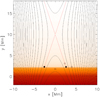 |
Fig. 1. Sketch of the initial state in the equilibrium represented by the distribution of gas pressure (in logarithmic scale) and magnetic field lines (black lines) along with the separatrices (red lines). The initial pressure pulses are depicted as two black full circles at separatrices at a height of 2.25 Mm above the photosphere, i.e. in the TR. The three unfilled black circles represent the detection points. |
Generally, the terms expressing the radiative losses Rloss, thermal conduction Tcond, and heating H should be added to the set of MHD equations. These terms are certainly important in building a realistic numerical model. However, at this stage when the wave and oscillatory processes are of primary interest, we neglect these terms.
2.3. Perturbations
At the start of the numerical simulation (t = 0 s), at two footpoints of the magnetic field structure, the equilibrium atmosphere is perturbed by an additional temperature (pressure) enhancement in the form
![Mathematical equation: $$ \begin{aligned} p = p_0 \Bigg \{1 + A_\mathrm{p} \sum _{i=1}^2 \exp {\Bigg [-\frac{(x-x_i^{\mathrm{P} })^2+(y-y^{\mathrm{P} })^2}{\lambda ^2} \Bigg ]} \Bigg \}, \end{aligned} $$](/articles/aa/full_html/2019/05/aa35188-19/aa35188-19-eq22.gif) (21)
(21)
where p0 is the initial gas pressure, Ap is the initial amplitude of the pressure pulse, λ = 0.1 Mm is the size of the pressure pulse, and  and yP are the positions of the initial perturbation pulses. The perturbation points are placed in
  Mm and
  Mm, respectively, with yP = 2.25 Mm for both points, which corresponds to the position in the TR (Fig. 1).
2.4. Numerical code
To solve the MHD Eqs. (1)–(4) we used the FLASH code, which is a well-tested, fully modular, parallel, multiphysics, open science simulation code that implements second- and third-order unsplit Godunov solvers with various slope limiters and Riemann solvers, as well as adaptive mesh refinement (AMR; Chung 2002). The Godunov solver combines the corner transport upwind method for multi-dimensional integration and the constrained transport algorithm for preserving the divergence-free constraint on the magnetic field (Lee & Deane 2009). We have used the minmod slope limiter and the Riemann solver (e.g., Toro 2006). The main advantage of using the AMR technique is to refine a numerical grid at steep spatial profiles, while keeping a grid coarse at the places where fine spatial resolution is not essential. In our case, the AMR strategy is based on controlling the numerical errors in a gradient of mass density that leads to the reduction of the numerical diffusion within the entire simulation region.
For our numerical simulations, we used a 2D Eulerian box of its width W = 20 Mm and height H = 20 Mm; we set the numerical box as ( − 10, 10) Mm × (−2,18) Mm in the x- and y- direction, respectively. The spatial resolution of the numerical grid was determined with the AMR method. We used the AMR grid with the minimum (maximum) level of the refinement blocks set to 3 (7). The whole simulation region was covered by 2962 blocks. Since every block consists of 8 × 8 numerical cells, this number of blocks corresponds to 189568 numerical cells and the smallest spatial resolution is Δx = Δy = 3.9 km.
At all boundaries, we fixed all plasma quantities to their equilibrium values using fixed-in-time boundary conditions, which lead only to negligibly small numerical reflections of incident wave signals.
3. Numerical results
Prior to running the numerical simulation, we verified that the system is in equilibrium for the adopted grid resolution by running the system without any pressure pulse. After this control test, we launched in the system two symmetric pressure pulses with the amplitudes of Ap = 10.0 in the points at  and yP (full black circles in Fig. 1). We took the amplitude Ap based on our previous simulations, where we found that during the pulse beam bombardment the transition region is rapidly heated due to the return-current effect (see the temperature profiles in Fig. 2 in Karlický & Henoux 1992), and the temperature enhancement depends on the chosen beam flux. Here we use Ap = 10.0 as an example in order to demonstrate the studied processes. Thus, the temperature at these points increases from the initial equilibrium value of Teq ≈ 0.17 MK to the temperature T ≈ 1.7 MK. We note that the perturbations we used are instantaneous, and thus mimic the heating caused by short-lasting particle beams. We based it on the hard X-ray flare emission (assumed to be generated by electron beams), which shows bursts lasting only a few seconds and e-folding times that are even shorter (Kane et al. 1980).
In Figs. 2–10 we show the results from our numerical simulations. For better readability and to see more details, Figs. 2–4 are shown within a range ( − 5, 5) Mm along the x-direction.
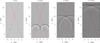 |
Fig. 2. Temporal evolution of changes in mass density Δ𝜚/𝜚0 at four different times, t = 2, 26, 64, and 106 s. The initial pressure pulse was launched in TR on separatrices (solid red lines). |
In Fig. 2 we show the time evolution of changes in the mass density Δ𝜚/𝜚0 for four different times, t = 2, 26, 64, and 106 s. The crossing of the red lines indicates the X-point of the magnetic reconnection. At a very early phase of this time evolution we can see that the shock wave, generated by the initial pressure pulse, propagates from both perturbation points symmetrically, and at time t = 26 s both wavefronts come across each other. Then both waves propagate towards the X-point (x = 0 Mm, y = 10 Mm), which they reach at time t = 64 s. At time t ≈ 106 s the waves come to the upper boundary of the presented region. It can also be seen that the waves propagate down to deeper layers of the solar atmosphere. These waves partially remain in the photosphere and deeper layers of solar body, and they are also partially reflected back with lower energy towards the higher altitudes in the solar atmosphere, which is clearly seen in Fig. 3.
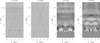 |
Fig. 3. Temporal evolution of changes in mass density Δ𝜚/𝜚0 at four different times, t = 300, 386, 410, and 460 s, showing the secondary wave generated by the oscillation of the photosphere. The wave is marked by the light green arrows; the red line represents the separatrices. |
In Fig. 3 we present the time evolution of changes in the mass density at later times, namely at t = 300, 386, 410 s, and t = 460 s. We can see here the waves reflected from the photosphere (y = 0 Mm), and the waves propagating down to even deeper layers and reflected later (see also right panels of Fig. 2 for times t = 64 s and t = 106 s). The reflected waves are marked by light green arrows. The figure at t = 300 s shows the wave shortly after the reflection from the photosphere. At time t = 386 s the reflected wave reaches the TR. After that time the wave continues in propagation to higher layers of the solar atmosphere, where we show two wavefronts at the time t = 410 s. The last shot presents the wave reaching the X-point at time t = 460 s.
Figure 4 presents again the time evolution of relative change of mass density for different times t = 530, 600, 640 s, and t = 690 s. As in Fig. 3, here we can see two waves triggered by oscillating photosphere (t = 530 s), whereas later in time t = 600 s the waves reach the TR. At time t = 640 s both wavefronts reach each other and continue in propagation higher to the solar atmosphere. At time t = 690 s they cross the X-point at height 10 Mm. The most important aspect of this set of pictures is that the initial pressure pulse triggers oscillations of the photosphere, thus generating waves propagating upwards where they can modulate quasi-periodically the process of the flare magnetic reconnection.
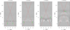 |
Fig. 4. Temporal evolution of changes of the mass density Δ𝜚/𝜚0 at four different times, t = 530, 600, 640, and 690 s, showing the second wave generated by the oscillation of the photosphere The wave is marked by the light green arrows; the red line represents the separatrices. |
In Figs. 5 and 6 we show the time-space plot of an evolution of the relative change of mass density Δ𝜚/𝜚0 along the y-axis for two values of x. In Fig. 5 it is along the axis of the symmetry of the magnetic structure, i.e. for x = 0 Mm, whereas Fig. 6 shows the plot through the perturbation point at x = 2.58 Mm. In both figures, at the beginning, we can see two shocks (from two spatially separated pulses) propagating upwards and downwards to higher and deeper layers of the solar atmosphere, respectively.
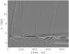 |
Fig. 5. Time-space plot showing the evolution of relative mass density change Δ𝜚/𝜚0 along the y-axis of symmetry of the magnetic structure at x = 0 Mm. |
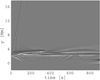 |
Fig. 6. Time-space plot showing the evolution of relative mass density change Δ𝜚/𝜚0 along the y-axis passing the perturbation point at x = 2.58 Mm. |
Arrival of the shocks is delayed because of the distance from the point of perturbation. The first shock propagates from the nearby perturbation point and the second one from the more distant perturbation point. The vertical velocity and the Mach number of the shock propagating upwards are vup ≈ 0.18 Mm s−1 and M ≈ 1.1, and those of the shock propagating downwards are vdown ≈ 0.011 Mm s−1 and M ≈ 1.5. The shock propagating to deeper layers of the solar atmosphere is partially reflected at approximately time t ≈ 200 s and changes to waves. Some waves also propagate below the photosphere to locations where they are later reflected. The wave above the photosphere reflects several times between TR and photosphere, and partially penetrates through TR and propagates upwards into the solar corona. Figure 6 is added for comparison. Here, the first shock starts without any delay because this plot presents an evolution along the line which comes through the perturbation point.
In Fig. 7 we show the time evolution of relative change of the mass density in the detection point located at the axis of the symmetry of the magnetic structure at y = 1.8 Mm (for the position of detection points, see Fig. 1). This figure presents another view of the shocks (two first peaks) and waves below the TR.
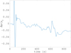 |
Fig. 7. Time evolution of relative mass density change Δ𝜚/𝜚0 at the detection point x = 0 Mm, y = 1.8 Mm. |
In Fig. 8 we present again the time evolution of relative changes of the mass density Δ𝜚/𝜚0, but for the point close to the initial perturbation point, x = 2.2 Mm, y = 3 Mm. This figure shows that shocks are generated during the pulse heating, and also that the plasma is evaporated. We can see that after first strong peak at t = 10 s, which corresponds to the shock generated in the nearby perturbation point, the second peak produced by the shock from the distant perturbation point appears at t = 50 s. This second peak is approximately two times lower than the first one (Δ = 0.1436/0.7637). Then at t = 166 s we observe a peak that is comparable to the previous one, but much broader. This peak shows an arrival of the evaporated plasma from the nearby perturbation point to the detection point (see also indication of the plasma evaporation in right panels of Fig. 2 for times t = 64 and 106 s.
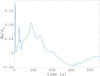 |
Fig. 8. Time evolution of relative mass density change Δ𝜚/𝜚0 at the point x = 2.2 Mm, y = 3.0 Mm. |
Figure 9 shows the time evolution of the density variation at the point x = 4.0 Mm and y = 2.25 Mm, which is located at the same altitude in TR as the perturbation point, but outside of it. This figure shows the wave propagating from the perturbation point through TR. This wave can correspond to the waves observed sometimes in Hα or UV. Using the wavelet analysis (Farge 1992; Torrence & Compo 1998), we estimated the period of this wave as about 174 s, see Fig. 10. This value is in very good agreement with the three-minute photospheric oscillations observed by the Solar Dynamics Observatory (SDO) Atmospheric Imaging Assembly (AIA), among others, and confirmed by numerical simulations (see e.g., Botha et al. 2011; Jelínek & Murawski 2013).
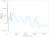 |
Fig. 9. Time evolution of relative mass density change Δ𝜚/𝜚0 at the point x = 4.0 Mm, y = 2.25 Mm. |
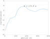 |
Fig. 10. Wavelet spectrum of the time profile presented in Fig. 9 showing the period 173.9 s. The red dashed line designates the cone of influence of the wavelet spectrum. |
4. Conclusions
In this paper we numerically studied shocks triggered by pressure pulses launched in the TR and consequently generated oscillations of deep atmospheric layers and waves propagating upwards which can modulate quasi-periodically the magnetic reconnection in solar flares. The model is based on the numerical solutions of MHD equations in two-dimensions, considering gravitationally stratified solar atmosphere with real temperature distribution according to the VAL-C model. Although the MHD model has limitations in the partly ionized photosphere and chromosphere, this model still plausibly demonstrates that the oscillations of photospheric layers, triggered by the pulse-beam heating, can produce quasi-periodically the upward-moving shocks and waves that can influence the magnetic reconnection in solar flares.
The period of oscillations found in the present model is about 174 s, which is in very good agreement with the well-known three-minute photospheric oscillations. The processes shown in this paper are a new possibility to explain some periodicity of solar flare emissions. It is a new alternative to the model with the resonating loop presented by Nakariakov et al. (2006). A question arises if there is any observational evidence that oscillations of deep layers of the solar atmosphere produce upward-propagating magnetoacoustic shocks or waves that modulate the magnetic reconnection, and thus periodically vary flare emissions. In this context it is very interesting that the upward-moving wave, presented in the paper by Liu et al. (2011), has the period 181 s.
From our computations it is evident that the processes presented in our paper need to be triggered by a very localized and strong pulse beam heating. The same trigger was also proposed as the mechanism that generates seismic waves (Kosovichev & Zharkova 1998; Zharkova & Zharkov 2007). Thus, we expect that the flares associated with the seismic waves could also be connected with the processes presented in this paper. We plan to analyse this possibility in a future work.
Acknowledgments
The authors thank the unknown referee for the constructive comments that improved the paper. P. J. and M. K. acknowledge the support from Grant 16-13277S of the Grant Agency of the Czech Republic. M. K. acknowledges the support from Grants 17-16447S, 18-09072S and 19-09489S of the Grant Agency of the Czech Republic. This work is based upon the activities of the international science team supported by the International Space Science Institute – Beijing, China. The authors also express their thanks to Professor Krzystof Murawski for the valuable discussions. P. J. thanks UMCS in Lublin for the financial support when he worked on this paper during his stay in June 2018. The FLASH code used in this work was developed by the DOE-supported ASC/Alliances Center for Astrophysical Thermonuclear Flashes at the University of Chicago. The wavelet analysis was performed using the software written by C. Torrence and G. Compo available at http://paos.colorado.edu/research/wavelets.
References
- Abbett, W. P., & Hawley, S. L. 1999, ApJ, 521, 906 [NASA ADS] [CrossRef] [Google Scholar]
- Allred, J. C., Hawley, S. L., Abbett, W. P., & Carlsson, M. 2005, ApJ, 630, 573 [NASA ADS] [CrossRef] [Google Scholar]
- Avrett, E. H., & Loeser, R. 2008, ApJS, 175, 229 [NASA ADS] [CrossRef] [Google Scholar]
- Botha, G. J. J., Arber, T. D., Nakariakov, V. M., & Zhugzhda, Y. D. 2011, ApJ, 728, 84 [NASA ADS] [CrossRef] [Google Scholar]
- Brown, J. C. 1971, Sol. Phys., 18, 489 [NASA ADS] [CrossRef] [Google Scholar]
- Chung, T. J. 2002, Computational Fluid Dynamics (Cambridge, UK: Cambridge University Press) [CrossRef] [Google Scholar]
- Farge, M. 1992, Annu. Rev. Fluid Mech., 24, 395 [Google Scholar]
- Fárník, F., Karlický, M., & Švestka, Z. 2003, Sol. Phys., 218, 183 [NASA ADS] [CrossRef] [Google Scholar]
- Fisher, G. H., Canfield, R. C., & McClymont, A. N. 1985a, ApJ, 289, 434 [NASA ADS] [CrossRef] [Google Scholar]
- Fisher, G. H., Canfield, R. C., & McClymont, A. N. 1985b, ApJ, 289, 425 [NASA ADS] [CrossRef] [Google Scholar]
- Fisher, G. H., Canfield, R. C., & McClymont, A. N. 1985c, ApJ, 289, 414 [NASA ADS] [CrossRef] [Google Scholar]
- Guo, M.-Z., Chen, S.-X., Li, B., Xia, L.-D., & Yu, H. 2016, Sol. Phys., 291, 877 [NASA ADS] [CrossRef] [Google Scholar]
- Hawley, S. L., & Fisher, G. H. 1994, ApJ, 426, 387 [NASA ADS] [CrossRef] [Google Scholar]
- Huang, J., Tan, B., Zhang, Y., Karlický, M., & Mészárosová, H. 2014, ApJ, 791, 44 [NASA ADS] [CrossRef] [Google Scholar]
- Jelínek, P., & Murawski, K. 2013, MNRAS, 434, 2347 [NASA ADS] [CrossRef] [Google Scholar]
- Jelínek, P., Karlický, M., & Murawski, K. 2015, ApJ, 812, 105 [NASA ADS] [CrossRef] [Google Scholar]
- Jelínek, P., Karlický, M., Van Doorsselaere, T., & Bárta, M. 2017, ApJ, 847, 98 [NASA ADS] [CrossRef] [Google Scholar]
- Kane, S. R., Crannell, C. J., Datlowe, D., et al. 1980, in Skylab Solar Workshop II, ed. P. A. Sturrock, 187 [Google Scholar]
- Karlický, M. 1990, Sol. Phys., 130, 347 [NASA ADS] [CrossRef] [Google Scholar]
- Karlický, M., & Henoux, J.-C. 1992, A&A, 264, 679 [NASA ADS] [Google Scholar]
- Karlický, M., & Jelínek, P. 2016, A&A, 590, A4 [NASA ADS] [CrossRef] [EDP Sciences] [Google Scholar]
- Karlický, M., Zlobec, P., & Mészárosová, H. 2010, Sol. Phys., 261, 281 [NASA ADS] [CrossRef] [Google Scholar]
- Kosovichev, A. G., & Zharkova, V. V. 1998, Nature, 393, 317 [NASA ADS] [CrossRef] [Google Scholar]
- Kupriyanova, E. G., Melnikov, V. F., Nakariakov, V. M., & Shibasaki, K. 2010, Sol. Phys., 267, 329 [NASA ADS] [CrossRef] [Google Scholar]
- Lee, D. 2013, J. Comput. Phys., 243, 269 [NASA ADS] [CrossRef] [Google Scholar]
- Lee, D., & Deane, A. E. 2009, J. Comput. Phys., 228, 952 [NASA ADS] [CrossRef] [Google Scholar]
- Liu, W., Title, A. M., Zhao, J., et al. 2011, ApJ, 736, L13 [NASA ADS] [CrossRef] [Google Scholar]
- MacNeice, P., Burgess, A., McWhirter, R. W. P., & Spicer, D. S. 1984, Sol. Phys., 90, 357 [NASA ADS] [CrossRef] [Google Scholar]
- Mariska, J. T., & Poland, A. I. 1985, Sol. Phys., 96, 317 [NASA ADS] [CrossRef] [Google Scholar]
- Mariska, J. T., Emslie, A. G., & Li, P. 1989, ApJ, 341, 1067 [NASA ADS] [CrossRef] [Google Scholar]
- McLaughlin, J. A., Nakariakov, V. M., Dominique, M., Jelínek, P., & Takasao, S. 2018, Space Sci. Rev., 214, 45 [NASA ADS] [CrossRef] [Google Scholar]
- Mészárosová, H., Karlický, M., Rybák, J., Fárník, F., & Jiřička, K. 2006, A&A, 460, 865 [NASA ADS] [CrossRef] [EDP Sciences] [Google Scholar]
- Nakariakov, V. M., Foullon, C., Verwichte, E., & Young, N. P. 2006, A&A, 452, 343 [NASA ADS] [CrossRef] [EDP Sciences] [Google Scholar]
- Nakariakov, V. M., Inglis, A. R., Zimovets, I. V., et al. 2010, Plasma Phys. Control. Fusion, 52, 124009 [NASA ADS] [CrossRef] [Google Scholar]
- Nakariakov, V. M., Pilipenko, V., Heilig, B., et al. 2016, Space Sci. Rev., 200, 75 [NASA ADS] [CrossRef] [Google Scholar]
- Nisticò, G., Pascoe, D. J., & Nakariakov, V. M. 2014, A&A, 569, A12 [NASA ADS] [CrossRef] [EDP Sciences] [Google Scholar]
- Parnell, C. E., Smith, J. M., Neukirch, T., & Priest, E. R. 1996, Phys. Plasmas, 3, 759 [NASA ADS] [CrossRef] [Google Scholar]
- Parnell, C. E., Neukirch, T., Smith, J. M., & Priest, E. R. 1997, Geophys. Astrophys. Fluid Dyn., 84, 245 [NASA ADS] [CrossRef] [Google Scholar]
- Pascoe, D. J. 2014, Res. Astron. Astrophys., 14, 805 [NASA ADS] [CrossRef] [Google Scholar]
- Priest, E. 2014, Magnetohydrodynamics of the Sun (Cambridge, UK: Cambridge University Press) [Google Scholar]
- Roberts, B., Edwin, P. M., & Benz, A. O. 1984, ApJ, 279, 857 [NASA ADS] [CrossRef] [Google Scholar]
- Solov’ev, A. A. 2010, Astron. Rep., 54, 86 [NASA ADS] [CrossRef] [Google Scholar]
- Takasao, S., & Shibata, K. 2016, ApJ, 823, 150 [NASA ADS] [CrossRef] [Google Scholar]
- Tan, B. 2008, Sol. Phys., 253, 117 [NASA ADS] [CrossRef] [Google Scholar]
- Toro, E. F. 2006, Int. J. Numer. Methods Fluids, 52, 433 [NASA ADS] [CrossRef] [Google Scholar]
- Torrence, C., & Compo, G. P. 1998, Bull. Am. Meteorol. Soc., 79, 61 [Google Scholar]
- Varady, M., Karlický, M., Moravec, Z., & Kašparová, J. 2014, A&A, 563, A51 [NASA ADS] [CrossRef] [EDP Sciences] [Google Scholar]
- Wang, T. J., Solanki, S. K., Innes, D. E., & Curdt, W. 2005, A&A, 435, 753 [NASA ADS] [CrossRef] [EDP Sciences] [Google Scholar]
- Zharkova, V. V., & Zharkov, S. I. 2007, ApJ, 664, 573 [NASA ADS] [CrossRef] [Google Scholar]
All Figures
|
Fig. 1. Sketch of the initial state in the equilibrium represented by the distribution of gas pressure (in logarithmic scale) and magnetic field lines (black lines) along with the separatrices (red lines). The initial pressure pulses are depicted as two black full circles at separatrices at a height of 2.25 Mm above the photosphere, i.e. in the TR. The three unfilled black circles represent the detection points. |
| In the text | |
|
Fig. 2. Temporal evolution of changes in mass density Δ𝜚/𝜚0 at four different times, t = 2, 26, 64, and 106 s. The initial pressure pulse was launched in TR on separatrices (solid red lines). |
| In the text | |
|
Fig. 3. Temporal evolution of changes in mass density Δ𝜚/𝜚0 at four different times, t = 300, 386, 410, and 460 s, showing the secondary wave generated by the oscillation of the photosphere. The wave is marked by the light green arrows; the red line represents the separatrices. |
| In the text | |
|
Fig. 4. Temporal evolution of changes of the mass density Δ𝜚/𝜚0 at four different times, t = 530, 600, 640, and 690 s, showing the second wave generated by the oscillation of the photosphere The wave is marked by the light green arrows; the red line represents the separatrices. |
| In the text | |
|
Fig. 5. Time-space plot showing the evolution of relative mass density change Δ𝜚/𝜚0 along the y-axis of symmetry of the magnetic structure at x = 0 Mm. |
| In the text | |
|
Fig. 6. Time-space plot showing the evolution of relative mass density change Δ𝜚/𝜚0 along the y-axis passing the perturbation point at x = 2.58 Mm. |
| In the text | |
|
Fig. 7. Time evolution of relative mass density change Δ𝜚/𝜚0 at the detection point x = 0 Mm, y = 1.8 Mm. |
| In the text | |
|
Fig. 8. Time evolution of relative mass density change Δ𝜚/𝜚0 at the point x = 2.2 Mm, y = 3.0 Mm. |
| In the text | |
|
Fig. 9. Time evolution of relative mass density change Δ𝜚/𝜚0 at the point x = 4.0 Mm, y = 2.25 Mm. |
| In the text | |
|
Fig. 10. Wavelet spectrum of the time profile presented in Fig. 9 showing the period 173.9 s. The red dashed line designates the cone of influence of the wavelet spectrum. |
| In the text | |
Current usage metrics show cumulative count of Article Views (full-text article views including HTML views, PDF and ePub downloads, according to the available data) and Abstracts Views on Vision4Press platform.
Data correspond to usage on the plateform after 2015. The current usage metrics is available 48-96 hours after online publication and is updated daily on week days.
Initial download of the metrics may take a while.