| Issue |
A&A
Volume 625, May 2019
|
|
|---|---|---|
| Article Number | A109 | |
| Number of page(s) | 10 | |
| Section | Extragalactic astronomy | |
| DOI | https://doi.org/10.1051/0004-6361/201834722 | |
| Published online | 22 May 2019 | |
The luminosity–volume test for cosmological fast radio bursts
1
Università di Bologna, Dip. di Fisica & Astronomia DIFA, Via Gobetti 92, Bologna, Italy
e-mail: This email address is being protected from spambots. You need JavaScript enabled to view it.
2
INAF – Istituto di Radioastronomia, Via Gobetti 92, Bologna, Italy
3
Università degli Studi di Milano-Bicocca, Dip. di Fisica “G. Occhialini”, Piazza della Scienza 3, 20126 Milano, Italy
4
INAF – Osservatorio Astronomico di Brera, Via Bianchi 46, 23807 Merate, Italy
5
INFN – Sezione di Milano Bicocca, Piazza della Scienza 3, 20126 Milano, Italy
Received:
26
November
2018
Accepted:
1
April
2019
Abstract
We have applied the luminosity–volume test, also known as ⟨V/Vmax⟩, to fast radio bursts (FRBs). We compare the 23 FRBs, recently discovered by ASKAP, with 20 of the FRBs found by Parkes. These samples have different flux limits and correspond to different explored volumes. We put constrains on their redshifts with probability distributions (PDFs) and applied the appropriate cosmological corrections to the spectrum and rate in order to compute the ⟨V/Vmax⟩ for the ASKAP and Parkes samples. For a radio spectrum of FRBs ℱν ∝ ν−1.6, we found ⟨V/Vmax⟩ = 0.68 ± 0.05 for the ASKAP sample, that includes FRBs up to z = 0.72+0.42−0.26, and 0.54 ± 0.04 for Parkes, that extends up to z = 2.1+0.47−0.38. The ASKAP value suggests that the population of FRB progenitors evolves faster than the star formation rate, while the Parkes value is consistent with it. Even a delayed (as a power law or Gaussian) star formation rate cannot reproduce the ⟨V/Vmax⟩ of both samples. If FRBs do not evolve in luminosity, the ⟨V/Vmax⟩ values of ASKAP and Parkes sample are consistent with a population of progenitors whose density strongly evolves with redshift as ∼z2.8 up to z ∼ 0.7.
Key words: methods: statistical / radio continuum: general
© ESO 2019
1. Introduction
Fast radio bursts (FRB) are very rapid (∼0.1–10 ms) and bright (∼0.1–1 Jy) radio pulses typically observed at ∼1 GHz frequency. Their detection is characterised by a frequency-dependent delay (∝ν−2) of the arrival time and a frequency-dependent broadening (∝ν−4) of the radio signal. These are typical signatures of a signal propagating through a low-density relativistic plasma. The signal dispersion is quantified by the dispersion measure (DM), proportional to the integral of the free electron density ne along the line-of-sight (LOS) from the observer to the source.
A collection of 52 FRBs has been made public through a database1 by Petroff et al. (2016). The large values of the observed dispersion measure DMobs (Lorimer et al. 2007; Thornton et al. 2013) and the detection of the host galaxy for the repeating FRB 121102 (Marcote et al. 2017), seem to favour their extra-galactic nature. The host galaxy redshift z ∼ 0.19 (Chatterjee et al. 2017; Tendulkar et al. 2017) is in fact consistent with the distance estimated from the observed DM. Despite the confirmed extra-galactic origin of this source, the fact that it remains the only repeater holds the possibility that it could be representative of a different class.
The “debate” on the origin of FRBs reminds much of the similar case of gamma ray bursts (GRBs; see Kulkarni 2018). Indeed, if extragalactic, FRBs have νLν luminosities around 1043 erg s−1 and energetics of the order of 1040 erg (Fig. 1).
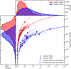 |
Fig. 1. Energy (νEν) as a function of redshift for FRBs detected by ASKAP (red circles) and Parkes (blue squares). The dashed lines correspond to the fluence limit for ASKAP and Parkes (red and blue respectively) obtained assuming the average FRB duration of the respective samples. Top and right panels: energy and redshift distributions of the two samples (same colour coding of the central plot). The thin curves represent, for each data point, the 1σ uncertainty on the energy produced by the uncertainty on the redshift. |
Such large energies and short durations imply a huge brightness temperature, of the order of TB ∼ 1034 − 1037 K. This in turn requires a coherent radiation process possibly originating from masers or compact bunches of emitting particles, as it has been recognised by many authors (Ghisellini 2017; Kumar et al. 2017; Yang & Zhang 2017; Ghisellini & Locatelli 2018; Katz 2018).
Many of the proposed progenitor theories of extragalactic FRBs include merging of compact objects such as neutron stars (Totani 2013); or white dwarfs (Kashiyama et al. 2013). FRBs could be flares from magnetars (Totani 2013; Thornton et al. 2013; Lyubarsky 2014; Beloborodov 2017) or giant pulses from pulsars (Cordes & Wasserman 2015), or they could be associated to the collapse of supra-massive neutron stars (Zhang 2014; Falcke & Rezzolla 2014); or dark matter induced collapse of neutron stars (Fuller & Ott 2015). See Platts et al. (2018), for an updated list of FRB theories.
A classical way to probe the unknown distance of a population of objects is through the ⟨V/Vmax⟩ test (also called luminosity–volume test). Firstly proposed by Schmidt (1968), the ⟨V/Vmax⟩ tests whether the distribution of objects is uniform within the volume of space defined by the observational selection criteria. Among other advantages, it is suitable for samples containing few objects and allows to combine samples of sources obtained with different selection criteria. Historically, it has been employed to study the space distribution of quasars and to assess the cosmic evolution of their population.
For a uniform population of sources with measured fluxes S, V/Vmax are the ratios of the volume V within which each source is distributed to the maximum volume Vmax within which each source could still be detected (which is individually defined by the sample selection flux limit). In an Euclidean space V/Vmax should be uniformly distributed between 0 and 1 with an average value ⟨V/Vmax⟩ = 0.5. Equivalently the cumulative source count distribution is N(> S)∝S−3/2.
The standard Euclidean approach to the luminosity–volume test has been performed on FRBs by different authors: Oppermann et al. (2016) find N(> S)∝S−n with 0.8 ≤ n ≤ 1.7; Caleb et al. (2016), report n = 0.9 ± 0.3 Li et al. (2017) find a much flatter population with n = 0.14 ± 0.20. More recently, James et al. (2019; hereafter J18), updated these results with 23 new FRBs (Shannon et al. 2018) discovered by the ASKAP array through the CRAFT survey (Macquart et al. 2010). They find n = 1.52 ± 0.24 for the combined ASKAP and Parkes FRB samples. However, for the first time, they compare different surveys with sufficient statistics, claiming a significant difference between the ASKAP CRAFT (n = 2.20 ± 0.47) and Parkes HTRU (n = 1.18 ± 0.24) surveys, respectively.
However, the assumption of a uniform distribution in Euclidean space for the number counts – ⟨V/Vmax⟩ test does not deal with the transient nature of FRBs. In this paper we performed the volume–luminosity test using the redshift estimated through the DM. We accounted for the possible uncertainty on z in terms of a probability density function (PDF) which encodes the uncertainties on (i) the Galactic free electron density model; (ii) the baryon distribution in the Inter-Galactic Medium (IGM) and (iii) the free electron density model of the FRB host environment. Furhtermore, we applied to each FRB the appropriate K-correction and accounted for the proper transformation from the observed to the intrinsic rate.
In Sect. 2 we present the two FRB samples used; in Sect. 3 we describe how to derive their ⟨V/Vmax⟩ accounting for their cosmological nature. A Monte Carlo approach is adopted to perform the ⟨V/Vmax⟩ for cosmological rate distributions (3.2) and compare with the real samples in Sect. 4. In Sect. 5 we discuss our results, and in Sect. 6 we draw our conclusions. We adopted a standard cosmology with Ωmax = 0.286, h = 0.696 and ΩΛ = 0.714.
2. Data samples
The ASKAP array of radio telescopes and the Parkes telescope provided two relatively large and well defined samples of FRBs which allow us to perform statistical analysis. From the online catalogue FRBCAT2 (Petroff et al. 2016), we collected all ASKAP and Parkes FRBs that have been confirmed via publication with a known signal-to-noise ratio (S/N) threshold.
2.1. ASKAP
We considered the 23 FRBs detected by ASKAP and recently published by Shannon et al. (2018) and Macquart et al. (2019). The ASKAP survey has an exposure of 5.1 × 10⁵ deg2 h, a field of view of 20 deg2 and a unique S/N threshold of 9.5 which corresponds to a limiting fluence of 23.16 × (wobs/1 ms)1/2 Jy ms (Shannon et al. 2018). Although FRB 171216 has been detected with a S/N = 8 in a single beam, it has a S/N = 10.3 considering its detection in the two adjacent beams (Shannon et al. 2018) and we then included this event in our sample.
The ASKAP sample is shown in Fig. 1 (red circles). To properly compare the energy density of FRBs at different redshifts we evaluated the energies at the observed frequency νobs = 1.3 GHz for all the FRBs. We applied the K-correction assuming an energy power law spectrum Eν ∝ ν−α with α = 1.6 (Macquart et al. 2019). Therefore the K-corrected energy density is given by Eq. (A.3), Eν(νobs) = Eν(νrest)(1 + z)α. The red dashed line corresponds to the ASKAP limiting fluence assuming the average intrinsic duration of the ASKAP sample ⟨wrest⟩ = 2.2 ms. The observed pulse duration (which defines the limiting curve – see above) scales as wobs = ⟨wrest⟩(1 + z). Because of the large field of view and the high fluence threshold, the ASKAP survey is more sensitive to nearer and relatively powerful events. This is evident in the redshift and energy distributions (top and left panels of Fig. 1) of the ASKAP sample whose mean values are ⟨z⟩ = 0.25 and ⟨E⟩ = 4.3 × 1041 erg respectively.
2.2. Parkes
Among all Parkes FRBs we found 20 verified events with known S/N threshold. In this case, since FRBs were detected in various surveys with different instrumental setups, the S/N threshold is not equal for all FRBs and therefore the corresponding fluence limit is not unique. The mean fluence limit of this sample results 0.54 × (wobs/1 ms)1/2 Jy ms and is represented by the dashed blue line in Fig. 1. Compared with ASKAP, the Parkes telescope is characterised by a smaller field of view (∼0.01 deg2) and a lower fluence limit being thus sensitive to more distant and less powerful events on average (cf. the distributions in the top and left panels of Fig. 1). The total exposure of the HTRU survey made at Parkes is 1441 deg2 h (Champion et al. 2016). The mean redshift and energy of the Parkes sample are ⟨z⟩ = 0.67 and ⟨E⟩ = 7.2 × 1040 erg, respectively.
The total sample includes 43 FRBs. When different data analyses for the same FRB were found, we chose the one computed with the method presented in Petroff et al. (2016) (if available) in order to build a uniform sample and because alternative searches tend to under-estimate the S/N (see Keane & Petroff 2015). Table 3 lists the galactic longitude and latitude (gl and gb), the observed dispersion measure (DMobs), the signal-to-noise ratio (S/N), the survey S/N threshold (S/Nlim), fluence ℱ(νobs), duration wobs and flux density S(νobs) all evaluated at the observed frequency νobs, the redshift calculated as presented in Sect. 3 and the references of the S/Nlim for all the 43 FRBs in our sample.
3. Method
Redshift information is necessary to perform the luminosity-volume test for a cosmological population of sources. In order to estimate z, Ioka (2003) and Inoue (2004) proposed a linear relation between the redshift and the dispersion measure due to the IGM (DMIGM):
 (1)
(1)
where C = 1200 pc cm−3. The redshift of a transient radio source can be estimated from the residual dispersion measure DMexcess, that is, once the Milky Way contribution is subtracted from the observed DMobs measured for the particular source:
 (2)
(2)
where DMhost is the dispersion measure of the host galaxy environment. The Milky Way dispersion measure DMMW is estimated in this work using the model of Yao et al. (2017; hereafter YMW16). The redshift of the source can be found from Eq. (2).
In principle, a large uncertainty on the redshift estimate is expected due to either the local environment and host galaxy free electron density and inclination (Xu & Han 2015; Luo et al. 2018) and to the high variance  of the unknown baryon halos and sub-structures along the LOS (McQuinn 2014; Dolag et al. 2015). In order to take into account these two sources of uncertainty – affecting DMhost and DMIGM respectively in Eq. (2) – we calculated the ⟨V/Vmax⟩ building appropriate probability functions for the redshifts PDF(z), rather than a unique value as obtained through Eq. (1).
Firstly we needed to model the host galaxy contribution DMhost. Xu & Han (2015) estimated DMhost for different galaxy morphologies and inclination angles i with respect to the LOS. In particular, for spiral galaxies they fitted skew normal functions f(DM, i) to the DMhost distributions for different values of the inclination angle i. We found the overall DMhost PDF (P(DMhost)) by averaging the functions f(DM, i), each weighted with the probability of the inclination angle sini. We extracted the DMhost values from P(DMhost). This allowed us to calculate the redshift zpeak, corresponding to the most probable value to be associated to the DMexcess of the jth FRB. The DM distribution of the host galaxy and environment has been also estimated by Luo et al. (2018). They obtained in general a smaller contribution of DMhost to the DMexcess than what derived by Xu & Han (2015). This is probably due to the simplistic but more conservative assumption of a MW, M 31-like galaxy as a host environment in the latter work, from which we derived the DMhost distribution.
The other source of uncertainty is related to the variance of DMIGM. This has been studied for example by McQuinn (2014) and Dolag et al. (2015). We considered the scenario giving the largest σDM(z) as reported in McQuinn (2014), obtained with a baryon (i.e. ne) distribution tracing the dark matter halos above a certain mass threshold. Although dedicated simulations show smaller uncertainties (McQuinn 2014; Dolag et al. 2015) we chose the most conservative σDM(z) relation, represented by the power-law function:
 (3)
(3)
where C1200 is the coefficient C in units of 1200 pc cm−3.
We calculated an inferior (zinf) and superior value (zsup) for the redshift in the PDF by introducing the left and right standard deviations σDM(z) respectively in the RHS of Eq. (2):
 (4)
(4)
 (5)
(5)
In the second equation a null DMhost contribution gives an upper limit to the redshift distribution. The PDF was then shaped as an asymmetric Gaussian: the peak of the PDF was assigned to the redshift zpeak; the left and right dispersion are σDM(zinf) = zpeak − zinf and σDM = zsup − zpeak respectively, where zinf < zpeak < zsup.
To calculate the Galactic contribution to the DM (DMMW) we considered two ne models: the NE2001 model (Cordes & Lazio 2001) and the model of YMW163. Assuming different models for the MW free electron contribution did not significantly affect the redshift distribution of the FRB sample. The same result has also been found by Luo et al. (2018) who also considered the presence of a free electron dark halo around the Milky Way. Its effect is found to be negligible however. This enabled us to base our analysis assuming one of the DM models without loosing generality. We considered the YMW16 as our baseline model.
Up to now we accounted for the stochastic dispersion around the DMIGM(z) relation. However, an additional source of uncertainty can systematically arise from the choice of the average DMIGM(z) relation, namely the C coefficient of Eq. (2). In fact simulations (Dolag et al. 2015) show a lower value than the one derived from modelling of the free electron density in the IGM. To account also for this systematic effect we calculated redshift uncertainties assuming different values of C in the range [950, 1200].
In general, large values of C decrease both the redshift z and the maximum observable redshift zmax, but by a slightly different amount, making the average ⟨V/Vmax⟩ to also decrease. However, the relative change of the ⟨V/Vmax⟩ values, for the C values considered, is limited to less than 3% for all spectral indexes. For semplicity, we thus assumed C = 1200.
3.1. ⟨V/Vmax⟩ of the FRB samples
The cosmological ⟨V/Vmax⟩ test is defined as the average over the sample of the ratios between the volume of space included within the source distance and the maximum volume in which an event, holding the same intrinsic properties, could have been observed. In terms of comoving distance D(z):
![Mathematical equation: $$ \begin{aligned} \left\langle \frac{V}{V_{\rm max}} \right\rangle = \frac{1}{N}\mathop \sum \limits _{i=0}^N \left[\frac{D^3(z)}{D_{\rm max}^3(z_{\rm max})}\right]_i, \end{aligned} $$](/articles/aa/full_html/2019/05/aa34722-18/aa34722-18-eq9.gif) (6)
(6)
where N is the total number of FRBs in one sample, D(z) and z are, respectively, the comoving distance and redshift of each object. Dmax and zmax are the same quantities that would be evaluated if that same source was observed at the limiting threshold of the same survey that found it, that is if its measured fluence ℱν (or S/N) coincided with the survey detection thresholds, ℱν, lim (or S/Nlim), assuming the same intrinsic properties of the event.
A large value of ⟨V/Vmax⟩ indicates sources distributed closer to the boundary of the volume probed by the given survey. Conversely, a low ⟨V/Vmax⟩ value indicates a population distributed closer to the observer with respect to the total survey-inspected volume.
The largest volume which can be probed  is uniquely defined by the survey (e.g. instrumental) parameters once a cosmology is assumed. It can be expressed in terms of the maximum possible redshift zmax at which a given source can be observed with the survey considered. In practice, we solved for zmax the equation (see Appendix A for the complete derivation):
![Mathematical equation: $$ \begin{aligned} \frac{D(z)}{D_{\rm max}(z_{\rm max})} = \left[ \frac{S/N_{\rm lim}}{S/N} \left(\frac{1+z}{1+z_{\rm max}}\right)^{-\frac{1}{2}-\alpha }\right]^\frac{1}{2} , \end{aligned} $$](/articles/aa/full_html/2019/05/aa34722-18/aa34722-18-eq11.gif) (7)
(7)
for each FRB in our sample. Here α is the observed spectral index of FRBs. Our formulation of the luminosity–volume test has been implemented for transient events embedded in a non-Euclidean cosmological volume and can be used with any user-defined luminosity function, source distribution, source spectral index and cosmology.
Following Shannon et al. (2018), we assumed a power-law spectrum for the whole FRB population, with non-evolving spectral index α. We considered three possible values of the spectral index α = 0, α = 1.6 (see Macquart et al. 2019) and α = 3 in order to test how the spectral slope affects the estimate of ⟨V/Vmax⟩. Redshift were obtained through a Monte-Carlo extraction, as described at the beginning of this section. By estimating zmax for each FRB we can computed ⟨V/Vmax⟩ for the two samples of ASKAP and Parkes FRBs and for the full combined ASKAP+Parkes sample. We then repeated the test 104 times to account for the stochastic uncertainty on redshift. Considering a spectral index of 1.6 as found by Macquart et al. (2019), we found ⟨V/Vmax⟩ = 0.681 ± 0.049 and ⟨V/Vmax⟩ = 0.538 ± 0.046 for ASKAP and Parkes, respectively, and ⟨V/Vmax⟩ = 0.624 ± 0.086 for the full sample. Values of ⟨V/Vmax⟩ for different values of the spectral index α are reported in Table 1.
⟨V/Vmax⟩ for different values of the spectral index α.
3.2. Comparison with simulated populations
We compared the values of the ⟨V/Vmax⟩ obtained for the ASKAP and Parkes samples with the ⟨V/Vmax⟩ expected for different cosmological population of sources. We tested three different redshift density distributions: (i) the cosmic star formation rate (Madau & Dickinson 2014; hereafter MD14); (ii) the short GRBs redshift distribution (as found by Ghirlanda et al. 2016; hereafter G16); (iii) a constant density distribution (i.e. no evolution).
We called “energy function” (EF) the density of sources (in the comoving volume) as a function of their radiated energy (in analogy with the luminosity function). For simplicity, we here neglected any EF evolution in cosmic time, considering only the density evolution corresponding to three cases above (Table 2).
⟨V/Vmax⟩ obtained at different ⟨z⟩ for populations extracted via the Monte Carlo method from the three tested redshift distributions described in the text.
Observational and instrumental parameters of FRBs in our sample.
Synthetic populations were generated through a Monte Carlo extraction from a PDF proportional to a given ψk(z) which represents the source density (i.e. per unit comoving volume) rate (i.e. per unit comoving time). The sub-scripts k = 1, 2, 3 refer to the three cases considered above. By accounting for the cosmological time dilation and volume, the sampling probability density function is:
 (8)
(8)
We then used the following procedure: we assumed a value of zmax as the maximum redshift at which a FRB population can be detected and generate a fake FRB sample from z = 0 to z = zmax. Then we evaluated the average ⟨V/Vmax⟩ and average ⟨z⟩ of the synthetic sample corresponding to that zmax. The ⟨V/Vmax⟩ calculated from these events was then assigned to the mean redshift ⟨z⟩ of the simulated FRBs. It became a point of the plotted curve in Fig. 2. We repeated this procedure for all values of zmax in order to obtain the model curves in Fig. 2.
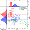 |
Fig. 2. ⟨V/Vmax⟩ of the ASKAP and Parkes FRB samples (red and blue squares, respectively) computed accounting for the cosmological terms (K-correction and rate) and the redshifts dispersion. Contours represent the 1-, 2- and 3-σ uncertainties on ⟨V/Vmax⟩. A spectral index α = 1.6 is assumed in this figure. Similar plots obtained with other possible values of the spectral index are shown in Fig. 3. The lines show the trends of ⟨V/Vmax⟩ as a function of increasing average redshift (i.e. survey depth). The different colours (styles) thick lines show the results of the evolution of ⟨V/Vmax⟩ obtained assuming different star formation rates (as labelled, see also Sect. 5). |
The value of zmax is linked to the value of the intrinsic energy of the FRB through Eq. (A.10), once the dependence of S/N on the energy, intrinsic duration and distance is made explicit (see Appendix A):
 (9)
(9)
where Dmax(zmax) is the proper distance at redshift zmax; Eν(νobs) is the energy density of the FRB at the observed frequency νobs ≃ 1.3 GHz. The constants A = 23.16 Jy ms for ASKAP and A = 0.54 Jy ms for Parkes specify the fluence limit of the two instruments:
![Mathematical equation: $$ \begin{aligned} F_{\rm lim}(\nu _{\rm obs}) = A \sqrt{\frac{{ w}_{\rm obs}\prime }{\mathrm{ms}}}\, = A \left(\frac{{ w}_{\rm rest}}{\mathrm{ms}}\right)^{1/2} (1+z_{\rm max})^{1/2}\,[\mathrm{Jy\, ms}] , \end{aligned} $$](/articles/aa/full_html/2019/05/aa34722-18/aa34722-18-eq57.gif) (10)
(10)
where  is the pulse duration we would observe if the FRB were located at redshift zmax. Therefore fixing zmax for a given extraction implies choosing the same intrinsic energy density Eν(νobs) for all FRBs of the fake sample generated according to that zmax.
We note that the resulting curve ⟨V/Vmax⟩ as a function of ⟨z⟩ is actually independent of the instrument (i.e. of the A parameter). In fact, if the A parameter is changed (namely, for different flux limits of the survey), at a given zmax the corresponding value of Eν(νobs) changes, but the curve remains the same.
4. Results
The ⟨V/Vmax⟩ test that we performed here includes the cosmological terms (K-correction and time dilation) arising from considering FRBs at cosmological distances as derived from their large observed dispersion measures. The ⟨V/Vmax⟩ for the FRB sample (ASKAP+Parkes) and individually for the two sub-samples (ASKAP and Parkes) are shown in Table 1 for different assumed spectral index α of the FRB intrinsic spectrum.
Figure 2 shows the ⟨V/Vmax⟩ values distributions, obtained from the Monte-Carlo extraction, as a function of the average redshift for the two samples for ASKAP and Parkes. Values obtained assuming different α are shown in Fig. 3. Solid contours show 1-, 2- and 3-σ level of confidence estimated via a bootstrap re-sampling of the FRB population’s redshift.
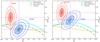 |
Fig. 3. Same as Fig. 2 where we assumed different FRB spectral index α. Left panel: α = 0; right panel: α = 3. |
The different curves show the expected ⟨V/Vmax⟩ as a function of mean redshift for the assumed density distributions (see Sect. 3.2). The extension of the curves before their respective turnover is due to the different redshift where the assumed density distributions peak (see also Fig. 4, bottom panel).
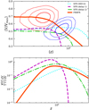 |
Fig. 4. Simulated populations obtained from different redshift density distributions ψk(z). Upper panel: ⟨V/Vmax⟩ as function of the average observable redshift. Contours show the ASKAP and Parkes confidence levels assuming α = 1.6 (see Fig. 2). Bottom panel: normalised source rate as function of redshift. Distributions are normalised to their integral. |
We find the values calculated for the sub-samples differing of Δ⟨V/Vmax⟩≃0.12. We note that they probe different volumes. The Parkes ⟨V/Vmax⟩ is fully consistent with a cosmic stellar population (CSFR – cyan solid line in Fig. 2) or its delayed version (dot-dashed green line in Fig. 2). The ASKAP sample instead deviates from the CSFR scenario. An evidence for the difference between the ASKAP and Parkes FRB populations has also been reported by J18, who find different slopes of the source count distribution for the two sub-samples. They also report the difference to be inconsistent with the one which is expected to be due to the different volumes probed by the two surveys.
The larger ⟨V/Vmax⟩ obtained for the ASKAP sample suggests a faster evolution with respect to the CSFR up to the distances currently explored by the ASKAP survey. This large value can not be explained even considering a delayed-CSFR (green dot-dashed line in Fig. 2) or a different spectral index for the FRB spectrum, nor a different DMIGM(z) relation. Overall, the ASKAP FRBs hint to a population of sources with a redshift density distribution different from those considered above (i.e. CSFR, delayed-CSFR as derived for short GRBs or constant formation rate).
5. Discussion
We have found that none of the population distributions adopted can account for the observed ⟨V/Vmax⟩. We demonstrate here that this result is independent of the particular shape of the energy function, as long as it does not evolve in cosmic time. In the procedure we have adopted, each point of the curves in Fig. 2 corresponds to a population of sources having the same energy, calculated in such a way that its fluence corresponds to the limiting fluence once the source is at its zmax. Smaller ⟨z⟩ correspond to less energetic sources.
In reality we have a distribution of energy, each corresponding to a different ⟨V/Vmax⟩, and ⟨z⟩. This pairs of values, however, belong to the shown curve. As an example, consider a specific EF, say a power law in energy N(E)∝E−Γ, with Γ positive. There will be many points at low energies, corresponding to smaller ⟨z⟩ for the curve in Fig. 2. Many sources at lower ⟨z⟩ means that the corresponding ⟨V/Vmax⟩ will be weighted more when calculating the final ⟨V/Vmax⟩. Still, the final value is constrained to be within the minimum and maximum values of the curve. As can be seen in Fig. 2 no curve can account for the ⟨V/Vmax⟩ of the ASKAP sample.
5.1. Cosmic star formation rate
Motivated by the strong hints on compact objects as sources of FRBs we considered a population with a rate density distribution described by the cosmic star formation:
 (11)
(11)
We adopted the parameters as reported by Madau & Dickinson (2014), a0 = 0.015, a1 = 2.7, a2 = 5.7, and zp = 1.9. For a1 > 0 and a2 > 1 the formation rate peaks at zp with an increasing rate, for z < zp, with slope a1. The ⟨V/Vmax⟩ as a function of ⟨z⟩ obtained with this function is shown in Fig. 2 (solid cyan line). The comparison with the ASKAP and Parkes values shows that a density evolution of FRBs following the star formation rate (Eq. (11)) is consistent with the Parkes ⟨V/Vmax⟩ value, but is largely below the ASKAP point (which is ∼3σ above the expectation for a population distributed as Eq. (11)).
5.2. Phenomenological “FRB formation rate”
The increase with redshift (∝(1 + z)p1 at low z) of the CSFR as represented by Eq. (11) is too shallow to account for the ASKAP point. In order to account for the values of ⟨V/Vmax⟩ of both the ASKAP and Parkes sub-samples we used the form:
 (12)
(12)
The large ⟨V/Vmax⟩ of ASKAP is found at an average redshift significantly smaller than the redshift where the CSFR peaks (see the bottom panel of Fig. 4). We have verified that we can reproduce both the ASKAP and the Parkes ⟨V/Vmax⟩ values using p0 = 1. p1 = 3.7, p2 = 4.8 and zp = 0.6. We stress that this does not correspond to a formal fit and other possible functional forms could well be consistent with the two points. Proper model selection and parameter fitting is out of the scope of the current work. Here we wanted to find an empirical density distribution which we can a-posteriori compared with the cosmic star formation rate.
The model described above is shown by the solid red line in Fig. 4 (top panel). For comparison, also the model curve obtained from the CSFR described in the previous section is shown (dotted cyan line).
5.3. Delayed cosmic star formation rate
One possibility (e.g. motivated by the similar case of short GRBs) is that the progenitors of FRBs produce the radio flashes at some advanced stage of their evolution. This would introduce a delayed density distribution which in the simplest case can be modelled starting from the CSFR as (see G16)
 (13)
(13)
For the delay function we considered (1) a normal PDF centred on 4 Gyr with a dispersion σ = 0.1 Gyr, and (2) a power-law with slope ∝τ−1 with a minimum delay equal to 1 Gyr. The latter is what is expected for the merging of compact objects (Greggio 2005; Belczynski et al. 2006; Mennekens et al. 2010; Ruiter et al. 2011; Mennekens & Vanbeveren 2016; Cao et al. 2018). The ⟨V/Vmax⟩ curves obtained with these two models are shown in Fig. 4 (top panel) by the dashed (magenta) and dot-dashed (green) lines, respectively. The resulting source rate are plotted in Fig. 4 (bottom panel) in purple and green colour respectively. Although they peak at later times by construction, none of the delay models look to be consistent with the ASKAP data. In fact the effect of the delay is just to move the maximum value attainable for the ⟨V/Vmax⟩ to later times (i.e. smaller redshifts), but does not increase enough to become consistent with the ASKAP value (cf. Fig. 4, upper panel).
6. Conclusions
We have performed the ⟨V/Vmax⟩ test for two different FRB samples, assuming that their distances are cosmological. Having characterised each sample through its average redshift, we have verified that the value of ⟨V/Vmax⟩ for the Parkes sample is similar to the one derived assuming that FRBs follow the star formation rate. This would indicate that FRBs can be associated to compact stars, such as neutron stars. Instead, for the ASKAP sample, sampling a closer volume but slightly more energetic FRBs, the value of ⟨V/Vmax⟩ is larger than the one derived with a population following the star formation rate. This result depends negligibly on the assumed FRB spectral index and has been determined accounting for the different sources of uncertainty on the estimate of the redshift of FRBs taking on a conservative approach.
At face value, this suggests that the progenitors of FRBs evolve in cosmic time faster than the star formation, and reach their maximum at redshift between the average redshift of the ASKAP and Parkes samples. Such fast evolution at relatively low redshifts can be due to a density evolution faster than the star formation rate, or to a luminosity (and energy) evolution superposed to a standard star formation rate. This is intriguing, because it would suggest a very peculiar population for the FRB progenitors, but at this stage we are not able to disentangle between these possibilities. A possibility is that, similarly to short Gamma Ray Bursts, there is a delay between the formation of the stars producing the FRB phenomenon and the FRB event. However, we verified that this cannot produce the steep rise (as a function of redshift) of event rate up to z ∼ 0.3–0.4 needed to account for the observed ASKAP ⟨V/Vmax⟩. The phenomenological “FRB formation rate” we have found, that can fit both the ASKAP and Parkes ⟨V/Vmax⟩ cannot be interpreted in a simple way on the basis of known population of sources. While the investigations of possibilities is demanded to a future work, we stress the need of having a survey exploring the same (large) sky area of ASKAP, but with a fluence limit comparable to Parkes. This will show how the FRB population evolves in time in the interesting 0.3–2 redshift range.
Fast Radio Burst Catalog (FRBCAT), http://frbcat.org/
Available at http://www.frbcat.org
Online calculators are available respectively at:
Acknowledgments
NL aknowledges financial support from the Horizon 2020 programme under the ERC Starting Grant “MAGCOW”, no. 714196. He also thanks F. Locatelli, A. Fasolini and S. Guadagna for useful and interesting discussions. G. Ghisellini and G. Ghirlanda aknowledge the PRIN-INAF 2017 “Towards the SKA and CTA era: discovery, localisation, and physics of transient sources”. We thank the anonymous referee for her/his critical comments that helped to improve the paper.
References
- Bannister, K. W., Shannon, R. M., Macquart, J.-P., et al. 2017, ApJ, 841, L12 [NASA ADS] [CrossRef] [Google Scholar]
- Bhandari, S., Keane, E. F., Barr, E. D., et al. 2018, MNRAS, 475, 1427 [NASA ADS] [CrossRef] [Google Scholar]
- Belczynski, K., Perna, R., Bulik, T., et al. 2006, ApJ, 648, 1110 [NASA ADS] [CrossRef] [Google Scholar]
- Beloborodov, A. M. 2017, ApJ, 843, L26 [NASA ADS] [CrossRef] [Google Scholar]
- Caleb, M., Flynn, C., Bailes, M., et al. 2016, MNRAS, 458, 708 [NASA ADS] [CrossRef] [Google Scholar]
- Cao, X.-F., Yu, Y.-W., & Zhou, X. 2018, ApJ, 858, 89 [NASA ADS] [CrossRef] [Google Scholar]
- Champion, D. J., Petroff, E., Kramer, M., et al. 2016, MNRAS, 460, L30 [NASA ADS] [CrossRef] [Google Scholar]
- Chatterjee, S., Law, C. J., Wharton, R. S., et al. 2017, Nature, 541, 58 [NASA ADS] [CrossRef] [Google Scholar]
- Cole, S., Norberg, P., Baugh, C. M., et al. 2001, MNRAS, 326, 255 [NASA ADS] [CrossRef] [Google Scholar]
- Cordes, J. M., & Lazio, T. J. W. 2001, ArXiv e-prints [arXiv:astro-ph/0207156] [Google Scholar]
- Cordes, J. M., & Wasserman, I. 2015, MNRAS, 457, 232 [Google Scholar]
- Dolag, K., Gaensler, B. M., Beck, A. M., & Beck, M. C. 2015, MNRAS, 451, 4277 [NASA ADS] [CrossRef] [Google Scholar]
- Falcke, H., & Rezzolla, L. 2014, A&A, 562, A137 [NASA ADS] [CrossRef] [EDP Sciences] [Google Scholar]
- Fuller, J., & Ott, C. D. 2015, MNRAS, 450, L71 [NASA ADS] [CrossRef] [Google Scholar]
- Ghirlanda, G., Salafia, O. S., Pescalli, A., et al. 2016, A&A, 594, A84 [NASA ADS] [CrossRef] [EDP Sciences] [Google Scholar]
- Ghisellini, G. 2017, MNRAS, 465, L30 [NASA ADS] [CrossRef] [Google Scholar]
- Ghisellini, G., & Locatelli, N. 2018, A&A, 613, A61 [NASA ADS] [CrossRef] [EDP Sciences] [Google Scholar]
- Greggio, L. 2005, A&A, 441, 1055 [NASA ADS] [CrossRef] [EDP Sciences] [Google Scholar]
- James, C. W., Ekers, R. D., Macquart, J.-P., Bannister, K. W., & Shannon, R. M. 2019, MNRAS, 483, 1342 [NASA ADS] [CrossRef] [Google Scholar]
- Kashiyama, K., Ioka, K., & Meszaros, P. 2013, ApJ, 776, L39 [NASA ADS] [CrossRef] [Google Scholar]
- Katz, J. I. 2017, MNRAS, 472, L85 [NASA ADS] [CrossRef] [Google Scholar]
- Katz, J. I. 2018, MNRAS, 481, 2946 [NASA ADS] [CrossRef] [Google Scholar]
- Keane, E. F., & Petroff, E. 2015, MNRAS, 447, 2852 [NASA ADS] [CrossRef] [Google Scholar]
- Keane, E. F., Stappers, B. W., Kramer, M., & Lyne, A. G. 2012, MNRAS, 425, L71 [NASA ADS] [CrossRef] [Google Scholar]
- Keane, E. F., Johnston, S., Bhandari, S., et al. 2016, Nature, 530, 453 [NASA ADS] [CrossRef] [Google Scholar]
- Keith, M. J., Jameson, A., van Straten, W., et al. 2010, MNRAS, 409, 619 [NASA ADS] [CrossRef] [Google Scholar]
- Kulkarni, S. R. 2018, Nat. Astron., 2, 832 [NASA ADS] [CrossRef] [Google Scholar]
- Kumar, P., Lu, W., & Bhattacharya, M. 2017, MNRAS, 468, 2726 [NASA ADS] [CrossRef] [Google Scholar]
- Inoue, S. 2004, MNRAS, 348, 999 [NASA ADS] [CrossRef] [Google Scholar]
- Ioka, K. 2003, ApJ, 598, L79 [NASA ADS] [CrossRef] [Google Scholar]
- Li, L.-B., Huang, Y.-F., Zhang, Z.-B., Li, D., & Li, B. 2017, Res. Astron. Astrophys., 17, 6 [NASA ADS] [CrossRef] [Google Scholar]
- Loeb, A., Shvartzvald, Y., & Maoz, D. 2014, MNRAS, 439, L46 [NASA ADS] [CrossRef] [Google Scholar]
- Lorimer, D. R., Bailes, M., McLaughlin, M. A., Narkevic, D. J., & Crawford, F. 2007, Science, 318, 777 [NASA ADS] [CrossRef] [PubMed] [Google Scholar]
- Lyubarsky, Y. 2014, MNRAS, 442, L9 [NASA ADS] [CrossRef] [Google Scholar]
- Luo, R., Lee, K., Lorimer, D. R., & Zhang, B. 2018, MNRAS, 481, 2320 [NASA ADS] [CrossRef] [Google Scholar]
- Macquart, J.-P., Bailes, M., Bhat, N. D. R., et al. 2010, PASA, 27, 272 [NASA ADS] [CrossRef] [Google Scholar]
- Macquart, J.-P., Shannon, R. M., Bannister, K. W., et al. 2019, ApJ, 872, L19 [NASA ADS] [CrossRef] [Google Scholar]
- Madau, P., & Dickinson, M. 2014, ARA&A, 52, 415 [NASA ADS] [CrossRef] [Google Scholar]
- Maoz, D., Loeb, A., Shvartzvald, Y., et al. 2015, MNRAS, 454, 2183 [NASA ADS] [CrossRef] [Google Scholar]
- Marcote, B., Paragi, Z., Hessels, J. W. T., et al. 2017, ApJ, 834, L8 [NASA ADS] [CrossRef] [Google Scholar]
- McQuinn, M. 2014, ApJ, 780, L33 [NASA ADS] [CrossRef] [Google Scholar]
- Mennekens, N., & Vanbeveren, D. 2016, A&A, 589, A64 [NASA ADS] [CrossRef] [EDP Sciences] [Google Scholar]
- Mennekens, N., Vanbeveren, D., de Greve, J., & de Donder, E. 2010, ASP Conf. Ser., 435 [Google Scholar]
- Oppermann, N., Connor, L. D., & Pen, U. L. 2016, MNRAS, 461, 984 [NASA ADS] [CrossRef] [Google Scholar]
- Oslowski, S., Shannon, R. M., Jameson, A., et al. ATel, 11396 [Google Scholar]
- Petroff, E., Bailes, M., Barr, E. D., et al. 2015, MNRAS, 447, 246 [NASA ADS] [CrossRef] [Google Scholar]
- Petroff, E., Barr, E. D., Jameson, A., et al. 2016, PASA, 33, e045 [NASA ADS] [CrossRef] [Google Scholar]
- Petroff, E., Burke-Spolaor, S., Keane, E. F., et al. 2017, MNRAS, 469, 4465 [NASA ADS] [Google Scholar]
- Platts, E., Weltman, A., Walters, A., et al. 2018, Phys. Rep., submitted [arXiv:1810.05836] [Google Scholar]
- Popov, S. B., & Postnov, K. A. 2010, in Proc. of the Conference dedicated to Viktor Ambartsumian’s 100th Anniversary, eds. H. A. Harutyunian, A. M. Mickaelian, & Y. Terzian (Yerevan: Publishing House of NAS RA), 129 [Google Scholar]
- Press, W. H., Flannery, B. P., & Teukolsky, S. A. 1986, Numerical Recipes. The Art of Scientific Computing (Cambridge: University Press) [Google Scholar]
- Price, R., et al. 2018, ATel, 11376 [Google Scholar]
- Ruiter, A. J., Belczynski, K., Sim, S. A., et al. 2011, MNRAS, 417, 408 [NASA ADS] [CrossRef] [Google Scholar]
- Schmidt, M. 1968, ApJ, 151, 393 [NASA ADS] [CrossRef] [Google Scholar]
- Scholz, P., Spitler, L. G., Hessels, J. W. T., et al. 2016, ApJ, 833, 177 [NASA ADS] [CrossRef] [Google Scholar]
- Shand, Z., Ouyed, A., Koning, N., & Ouyed, R. 2016, Res. Astron. Astrophys., 16, 80 [NASA ADS] [CrossRef] [Google Scholar]
- Shannon, R. M., Macquart, J.-P., Bannister, K. W., et al. 2018, Nature, 562, 386 [NASA ADS] [CrossRef] [Google Scholar]
- Spitler, L. G., Cordes, J. M., Hessels, J. W. T., et al. 2014, ApJ, 790, 101 [NASA ADS] [CrossRef] [Google Scholar]
- Tendulkar, S. P., Bassa, C. G., Cordes, J. M., et al. 2017, ApJ, 834, L7 [NASA ADS] [CrossRef] [Google Scholar]
- Thornton, D., Stappers, B., Bailes, M., et al. 2013, Science, 341, 53 [NASA ADS] [CrossRef] [PubMed] [Google Scholar]
- Totani, T. 2013, PASJ, 65, L12 [NASA ADS] [CrossRef] [Google Scholar]
- Xu, J., & Han, J. L. 2015, Res. Astron. Astrophys., 15, 1629 [NASA ADS] [CrossRef] [Google Scholar]
- Yang, Y. P., & Zhang, B. 2017, ApJ, 868, 31 [Google Scholar]
- Yao, J. M., Manchester, R. N., & Wang, N. 2017, ApJ, 835, 29 [NASA ADS] [CrossRef] [Google Scholar]
- Zhang, B. 2014, ApJ, 780, L21 [NASA ADS] [CrossRef] [Google Scholar]
Appendix A: Complete derivation of the cosmological ⟨V/Vmax⟩ test
A.1. ⟨V/Vmax⟩ value estimation
The V/Vmax computed in this work (Eq. (7)), which accounts for the cosmological k-correction and proper rate of transient FRBs, is derived as follows. We considered the relation:
 (A.1)
(A.1)
where we used the relation between luminosity distance and proper distance: DL = (1 + z)D. Analogously:
 (A.2)
(A.2)
where Eν is the intrinsic energy density, νe = νobs(1 + z) and ν′e = νobs(1 + zmax) are the emitted frequencies at proper distances D(z) and Dmax(zmax), respectively.
We assumed that FRBs have a power-law energy spectrum spectral slope α, at least in a frequency range comparable to that probed by the observer frame frequency νobs ≃ 1.3 GHz. Therefore, we could write:
 (A.3)
(A.3)
Combining Eqs. (A.1), (A.2) and (A.3) we obtained:
![Mathematical equation: $$ \begin{aligned} \frac{D(z)}{D_{\rm max}(z_{\rm max})} = \left[ \frac{F_{\rm lim}(\nu _{\rm obs})}{F(\nu _{\rm obs})} \left( \frac{1+z}{1+z_{\rm max}}\right)^{-\alpha }\right]^{1/2}. \end{aligned} $$](/articles/aa/full_html/2019/05/aa34722-18/aa34722-18-eq65.gif) (A.4)
(A.4)
From the antenna equation, the signal-to-noise ratio of an event of duration wobs is defined as:
 (A.5)
(A.5)
where G is the antenna gain, NP is the number of polarizations, η is the efficiency and Tsys is the antenna temperature. The S/N can also be described in terms of the fluence ℱ(ν) = S(ν) wobs as:
 (A.6)
(A.6)
The limiting threshold over which an FRB is detected can also be described in terms of S/N:
 (A.7)
(A.7)
where  ; all the parameters related to the observing conditions/setup (G, NP, Δν, η and Tsys) are the same when we want to look for the maximum distance at which the FRB could be observed. However, the observed duration of the transient event changes with redshift. We thus related the ratios of observed and threshold values with a function of their redshifts:
 (A.8)
(A.8)
Through Eq. (A.8) w recast Eq. (A.4) in terms of the S/N with respect to S/Nlim
![Mathematical equation: $$ \begin{aligned} \frac{D(z)}{D_{\rm max}(z_{\rm max})} = \left[ \frac{S/N_{\rm lim}}{S/N} \left(\frac{1+z}{1+z_{\rm max}}\right)^{-\frac{1}{2}-\alpha }\right]^\frac{1}{2} , \end{aligned} $$](/articles/aa/full_html/2019/05/aa34722-18/aa34722-18-eq71.gif) (A.9)
(A.9)
retrieving Eq. (7). Equivalently one can write it as
 (A.10)
We put in the right-hand side (RHS) of Eq. (A.10) all the terms depending on zmax. We defined the function Υ(zmax) as the RHS. Υ(zmax) can be evaluated using the left-hand side (LHS) of the same equation, that is, combining the observed, instrumental and cosmological information. If the functions Dmax(z) and Υ(z) are invertible one can in principle solve the above equation for zmax. We note that only for α > −1/2 this function is monotonic and invertible. Under this assumption
![Mathematical equation: $$ \begin{aligned} z_{\rm max} = \Upsilon ^{-1} \left[\frac{S/N}{S/N_{\rm lim}} \, D^2(z) \, (1+z)^{\frac{1}{2}+\alpha } \right]. \end{aligned} $$](/articles/aa/full_html/2019/05/aa34722-18/aa34722-18-eq73.gif) (A.11)
(A.11)
The function Υ depends on cosmology through the definition of D(z)
 (A.12)
and from the spectral index α of the intrinsic FRB specific luminosity.
The estimates of the spectral index is given considering the 23 ASKAP burst signals (Shannon et al. 2018) detected with narrow-band (336 MHz) centred at 1.32 GHz showing intense fine-scale features (Macquart et al. 2019). They calculate a mean spectral index  . This represents the current best (and only) estimate of the spectral index for the non-repeating FRBs, as far as any broad-band information will be given.
The analytic form of Eq. (A.11) is not straightforward to obtain so we solved it numerically.
A.2. S/N and S/Nlim
The fact itself that in Eq. (A.11) the ratio between a threshold and the corresponding observed quantity are present (instead of just the observed one) removes the dependency of the test from any survey parameter, since they would play the same role in the definition of both terms in the ratio. The fact that the ratio between observed and threshold S/N is independent of the survey area and time coverage or any other observation parameter has been previously proven by J18 in a rigorous way. Our derivation can be helpful in giving an intuitive and straightforward proof of the fact.
The (S/N)/(S/N)lim approach has also the advantage that any other quantity which varies linearly with the fluence ℱ(ν) can be used in its place in Eq. (A.11). The smartest choice is to use the S/N, which is the ratio between the amplitude of the time-integrated FRB signal (after the noise level being normalised to 0) and the standard deviation of the noise in the continuum (Petroff et al. 2016).
We chose to use S/N as S/Nlim is the quantity which is actually defined in a survey in order to claim a detection, rather than the flux density Sν or the fluence ℱν. Moreover, the way the S/N is defined is in principle independent from the pulse broadening effect whenever a signal is detected. In fact, highly-broadened signals could not be recognised as FRB candidates by searching pipelines, but a non-detection does not affect the completeness of the sample in a ⟨V/Vmax⟩ test.
All Tables
⟨V/Vmax⟩ obtained at different ⟨z⟩ for populations extracted via the Monte Carlo method from the three tested redshift distributions described in the text.
All Figures
|
Fig. 1. Energy (νEν) as a function of redshift for FRBs detected by ASKAP (red circles) and Parkes (blue squares). The dashed lines correspond to the fluence limit for ASKAP and Parkes (red and blue respectively) obtained assuming the average FRB duration of the respective samples. Top and right panels: energy and redshift distributions of the two samples (same colour coding of the central plot). The thin curves represent, for each data point, the 1σ uncertainty on the energy produced by the uncertainty on the redshift. |
| In the text | |
|
Fig. 2. ⟨V/Vmax⟩ of the ASKAP and Parkes FRB samples (red and blue squares, respectively) computed accounting for the cosmological terms (K-correction and rate) and the redshifts dispersion. Contours represent the 1-, 2- and 3-σ uncertainties on ⟨V/Vmax⟩. A spectral index α = 1.6 is assumed in this figure. Similar plots obtained with other possible values of the spectral index are shown in Fig. 3. The lines show the trends of ⟨V/Vmax⟩ as a function of increasing average redshift (i.e. survey depth). The different colours (styles) thick lines show the results of the evolution of ⟨V/Vmax⟩ obtained assuming different star formation rates (as labelled, see also Sect. 5). |
| In the text | |
|
Fig. 3. Same as Fig. 2 where we assumed different FRB spectral index α. Left panel: α = 0; right panel: α = 3. |
| In the text | |
|
Fig. 4. Simulated populations obtained from different redshift density distributions ψk(z). Upper panel: ⟨V/Vmax⟩ as function of the average observable redshift. Contours show the ASKAP and Parkes confidence levels assuming α = 1.6 (see Fig. 2). Bottom panel: normalised source rate as function of redshift. Distributions are normalised to their integral. |
| In the text | |
Current usage metrics show cumulative count of Article Views (full-text article views including HTML views, PDF and ePub downloads, according to the available data) and Abstracts Views on Vision4Press platform.
Data correspond to usage on the plateform after 2015. The current usage metrics is available 48-96 hours after online publication and is updated daily on week days.
Initial download of the metrics may take a while.