© ESO 2019

1. Introduction

The theory of thermal instabilities dates back to the famous papers written by Field (1965) and Parker (1953). The former made a very detailed analysis of the thermal instability mechanism in an infinite homogeneous medium and explained how such an instability can originate from catastrophic radiative cooling effects. This analysis was then extended to include non-uniform media, both in relatively simple slab configurations (Van der Linden & Goossens 1991a; Van der Linden et al. 1992) as in cylindrical equilibrium models with coronal conditions (Van der Linden & Goossens 1991b; Ireland et al. 1995; Soler et al. 2011). It was soon proposed that this route through thermal instability could be responsible for the formation of solar prominences (Smith & Priest 1977; Priest & Smith 1979), and that non-adiabatic effects like thermal conduction across magnetic field lines and resistivity may play an important role in the development of prominence fine structure (Van der Linden & Goossens 1991b; Ireland et al. 1998).

The optically thin radiative losses themselves are dependent on temperature and density, and over the years various works have resulted in accurate cooling curves (Dalgarno & McCray 1972; Mellema & Lundqvist 2002; Colgan et al. 2008; Schure et al. 2009) that give the radiative loss as a function of temperature. In coronal physics for example, the cooling curve proposed by Rosner et al. (1978) is widely used.

The plasma in the solar corona can be assumed to be in a thermal equilibrium, realising a delicate and as yet partially understood balance between radiative losses and heating. If these losses increase with decreasing temperature, a small initial perturbation of the equilibrium state is enough to trigger a catastrophic runaway cooling reaction. Any drop in temperature will increase the energy losses via an increase in radiative cooling, and the plasma will start to cool down. This can lead to a pressure gradient, resulting in movement of material along magnetic field lines to try and restore pressure equilibrium. The local increase in density further increases the radiative losses (as these are dependent on density squared), which in turn decreases the temperature even more. This results in a catastrophic runaway effect, characterised by a rapid drop in temperature and a strong increase in density. If this process happens at the top of a magnetic arcade it can give rise to the formation of condensed regions, eventually resulting in a solar prominence as shown for example by Hildner (1974) and Drake et al. (1993).

Numerical modelling of radiative condensations started out in 1D simulations, essentially using hydrodynamics along fixed field line shapes with the inclusion of chromospheric heating (Mok et al. 1990; Antiochos et al. 1999; Karpen et al. 2001; Müller et al. 2003, 2004, 2005; Luna et al. 2012; Xia et al. 2011). Some early 2.5D simulations of prominence formation were done by Choe & Lee (1992) where the onset of thermal instability was triggered by the injection of chromospheric plasma into the coronal loop, resulting from syphon-type upflows due to photospheric shearing motions. These models did not include chromospheric regions however. The first 2.5D simulation that realistically simulated the onset and formation of a solar prominence was done by Xia et al. (2012), where an evaporation–condensation mechanism was used to evaporate chromospheric material into the solar corona leading to a density increase, eventually forming condensations due to the trigger of thermal instabilities as a result of runaway radiative cooling effects.

The dynamical evolution of a prominence was further explored by Keppens & Xia (2014) and Moschou et al. (2015) for example, showing the coronal rain phenomenon in their simulations, while Kaneko & Yokoyama (2015) performed additional models of flux-rope formation and radiative condensation. Xia & Keppens (2016) reported the first fully 3D model of a solar prominence in realistic solar coronal conditions, demonstrating a corona–chromosphere plasma cycle yielding a continuous formation of condensations. Recent works further investigate this coronal rain phenomenon, in particular Xia et al. (2017), as well as simulations of prominence eruptions formed through runaway radiative cooling (Fan 2018). Kaneko & Yokoyama (2017) on the other hand adopted a 3D condensation–reconnection model, where they showed that magnetic reconnection near a polarity inversion line of a coronal arcade cannot only create a flux rope that sustains a solar prominence, but can also trigger runaway radiative cooling.

Peng & Matsumoto (2017) showed that the thermal-instability mechanism can be responsible for the formation of molecular loops in the galactic central region. Furthermore, Wareing et al. (2016) found that the same process can explain the appearance of higher-density filaments in star-forming clouds. Ji et al. (2018) proposed that the cold gas found in galactic haloes can originate from in situ condensation through thermal instability, while Fragile et al. (2018) found evidence of thermal instability in thin disks accreting onto stellar-mass black holes, eventually leading to the subsequent vertical collapse of the disk. All of the above is a clear indication that the theory of thermal instabilities is not only relevant in solar coronal applications, but is widely applicable in various other astrophysical domains as well, such that acquiring a deep understanding of thermal instabilities is important. Recently, Waters & Proga (2018) surveyed all possible regimes of thermal instability in hydrodynamics, investigating the stability of acoustic and condensation modes between the two wavelength limits of isobaric and isochoric instability.

The temporal evolution of a thermal instability eventually becomes a non-linear process, such that later stages can only be researched by numerical simulations. However, our main aim of this paper is to demonstrate that when the simulations are initialized in the right manner and accurately capture the thermodynamical processes, there is good correspondence between theory and simulations. The dispersion relation calculated by linearizing the non-adiabatic magnetohydrodynamic (MHD) equations gives us complete knowledge of the different wave modes propagating in a plasma. Using the standard Fourier representation of eigenfrequencies ω, the non-adiabatic effects render the solutions complex, such that the imaginary part indicates either damping (stability) or growth (overstability) of the wave amplitude.

As we show in sect. 5 this wave damping is fully reproduced in the simulations of damped slow waves, with a damping rate consistent with the theoretical predictions taking observed thermodynamical constraints (like isobaric or isochoric processes) into account. The (non-linear) onset of thermal instability, characterised by a sudden increase in wave amplitude also shows good correspondence with the growth rate predicted by the thermal mode solution from linear theory. Even when going into more complex configurations, such as the interaction between multiple waves (Sect. 6), we see that this is still the case. This puts us in a position where we can predict growth or damping rates with reasonable accuracy, even in the non-linear regime of thermal instability formation.

2. Governing equations

2.1. Linearization and dispersion relation

We start by writing down the MHD equations in which we neglect resistivity, gravity, conduction, and other non-adiabatic effects, except for a radiative cooling contribution. These are given by

$$\begin{array}{cc}\hfill \frac{\partial \rho }{\partial t}& +\mathrm{\nabla }·(\rho \mathit{v})=0,\hfill \end{array}$$(1)

$$\begin{array}{cc}\hfill \rho \frac{\partial \mathit{v}}{\partial t}& +\rho \mathit{v}·\mathrm{\nabla }\mathit{v}+(\gamma -1)\mathrm{\nabla }(\rho e)+(\mathrm{\nabla }\mathit{B})·\mathit{B}-\mathit{B}·\mathrm{\nabla }\mathit{B}=0,\hfill \end{array}$$(2)

$$\begin{array}{cc}\hfill \frac{\partial e}{\partial t}& +\mathit{v}·\mathrm{\nabla }e+(\gamma -1)e\mathrm{\nabla }·\mathit{v}+\rho \mathcal{L}=0,\hfill \end{array}$$(3)

$$\begin{array}{cc}\hfill \frac{\partial \mathit{B}}{\partial t}& +\mathit{v}·\mathrm{\nabla }\mathit{B}+\mathit{B}\mathrm{\nabla }·\mathit{v}-\mathit{B}·\mathrm{\nabla }\mathit{v}=0,\mathrm{\nabla }·\mathit{B}=0,\hfill \end{array}$$(4)

with the magnetic field in units where μ₀ = 1, and ℒ is the heat-loss function, defined as energy losses minus energy gains due to radiative cooling effects (Field 1965). The quantities ρ, v, B, and e are the density, velocity, magnetic field, and internal energy, respectively. The latter is defined as

$$\begin{array}{c}\hfill e=\frac{p}{\rho (\gamma -1)},\end{array}$$(5)

where p denotes the thermal pressure. The ratio of specific heats is given by γ, taken to be 5/3. The system is closed using the ideal gas law

$$\begin{array}{c}\hfill p\mu =\mathcal{R}\rho T,\end{array}$$(6)

where T, μ, and ℛ represent the temperature, mean molecular weight, and gas constant, respectively. The next step is to linearize these equations assuming an infinite, homogeneous, and time-independent background (meaning ∂_t = 0 and there are no gradients in the equilibrium quantities). This background is denoted here by ρ₀, v₀ = 0, B₀, p₀ and e₀, while the deviations from equilibrium are denoted with a subscript “1”. This results in the following linearized system of equations

$$\begin{array}{cc}\hfill \frac{\partial {\rho }_1}{\partial t}& +{\rho }_0\mathrm{\nabla }·{\mathit{v}}_1=0,\hfill \end{array}$$(7)

$$\begin{array}{cc}\hfill {\rho }_0\frac{\partial {\mathit{v}}_1}{\partial t}& +(\gamma -1)(e_0\mathrm{\nabla }{\rho }_1+{\rho }_0\mathrm{\nabla }{e}_1)\hfill \\ \hfill & +(\mathrm{\nabla }{\mathit{B}}_1)·{\mathit{B}}_0-{\mathit{B}}_0·\mathrm{\nabla }{\mathit{B}}_1=0,\hfill \end{array}$$(8)

$$\begin{array}{cc}\hfill \frac{\partial e_1}{\partial t}& +(\gamma -1)e_0\mathrm{\nabla }·{\mathit{v}}_1+{\rho }_0({\mathcal{L}}_{\mathrm{T}}{T}_1+{\mathcal{L}}_{\rho }{\rho }_1)=0,\hfill \end{array}$$(9)

$$\begin{array}{cc}\hfill \frac{\partial {\mathit{B}}_1}{\partial t}& +{\mathit{B}}_0\mathrm{\nabla }·{\mathit{v}}_1-{\mathit{B}}_0·\mathrm{\nabla }{\mathit{v}}_1=0,\mathrm{\nabla }·{\mathit{B}}_1=0.\hfill \end{array}$$(10)

The quantities ℒ_T and ℒ_ρ denote the temperature and density derivatives of the heat-loss function, defined as

$$\begin{array}{c}\hfill {\mathcal{L}}_{\mathrm{T}}\equiv {\frac{\partial \mathcal{L}}{\partial T}|}_{\rho }\mathrm{and}{\mathcal{L}}_{\rho }\equiv {\frac{\partial \mathcal{L}}{\partial \rho }|}_{\mathrm{T}},\end{array}$$(11)

to be evaluated using the equilibrium quantities. The linearized expressions for the internal energy and ideal gas law allow us to solve for T₁, such that we can rewrite T₁ as a function of e₁ and equilibrium quantities:

$$\begin{array}{c}\hfill T_1=\frac{T_0}{e_0}{e}_1,\end{array}$$(12)

which is in turn used to substitute T₁ in the linearized energy Eq. (9). Subsequently, we assume plane-wave solutions of the form

$$\begin{array}{c}\hfill {\rho }_1=\widehat{\rho }{\mathrm{e}}^{i(\mathit{k}·\mathit{r}-\omega t)},\end{array}$$(13)

such that we obtain a system of eigenvalue equations, given by

$$\begin{array}{cc}\hfill \omega \widehat{\rho }& ={\rho }_0\mathit{k}·\widehat{\mathit{v}},\hfill \end{array}$$(14)

$$\begin{array}{cc}\hfill \omega {\rho }_0\widehat{\mathit{v}}& =(\gamma -1)(e_0\mathit{k}\widehat{\rho }+{\rho }_0\mathit{k}\widehat{e})+\mathit{k}(\widehat{\mathit{B}}·{\mathit{B}}_0)-({\mathit{B}}_0·\mathit{k})\widehat{\mathit{B}},\hfill \end{array}$$(15)

$$\begin{array}{cc}\hfill \omega \widehat{e}& =(\gamma -1)e_0\mathit{k}·\widehat{\mathit{v}}-\frac{{\rho }_0{T}_0}{e_0}{\mathcal{L}}_{\mathrm{T}}i\widehat{e}-{\rho }_0{\mathcal{L}}_{\rho }i\widehat{\rho },\hfill \end{array}$$(16)

$$\begin{array}{cc}\hfill \omega \widehat{\mathit{B}}& ={\mathit{B}}_0(\mathit{k}·\widehat{\mathit{v}})-({\mathit{B}}_0·\mathit{k})\widehat{\mathit{v}},\hfill \end{array}$$(17)

which revisits the derivations done by Field (1965). Following the general results in Goedbloed & Poedts (2004) we choose B₀ along the z-axis and k in the x-z plane:

$$\begin{array}{c}\hfill {\mathit{B}}_0=(0,0,B_0)\mathrm{and}\mathit{k}=(k_{\perp },0,k_{\Vert }),\end{array}$$(18)

with k_⊥ and k_∥ the components of k perpendicular and parallel to the magnetic field lines, respectively. This can in turn be used to rewrite Eq. (17) in its respective components, yielding

$$\begin{array}{c}\hfill \widehat{\mathit{B}}=-\frac{1}{\omega }{k}_{\Vert }{B}_0{\widehat{v}}_x{\widehat{\mathit{e}}}_x-\frac{1}{\omega }{k}_{\Vert }{B}_0{\widehat{v}}_y{\widehat{\mathit{e}}}_y+\frac{1}{\omega }{k}_{\perp }{B}_0{\widehat{v}}_x{\widehat{\mathit{e}}}_z,\end{array}$$(19)

where ${\widehat{v}}_x$ denotes the $\widehat{\mathit{v}}$ component in the x-direction and ê_x, ê_y, ê_z are the unit vectors in the x, y and z directions, respectively. Using this to eliminate $\widehat{\mathit{B}}$ from the equation of motion results in

$$\begin{array}{cc}\hfill \omega {\rho }_0{\widehat{v}}_x& =(\gamma -1)e_0{k}_{\perp }\widehat{\rho }+(\gamma -1){\rho }_0{k}_{\perp }\widehat{e}+\frac{1}{\omega }{k}^2{B}_0^2{\widehat{v}}_x,\hfill \end{array}$$(20)

$$\begin{array}{cc}\hfill \omega {\rho }_0{\widehat{v}}_y& =\frac{1}{\omega }{k}_{\Vert }^2{B}_0^2{\widehat{v}}_y,\hfill \end{array}$$(21)

$$\begin{array}{cc}\hfill \omega {\rho }_0{\widehat{v}}_z& =(\gamma -1)e_0{k}_{\Vert }\widehat{\rho }+(\gamma -1){\rho }_0{k}_{\Vert }\widehat{e}.\hfill \end{array}$$(22)

We see that ${\widehat{v}}_y$ is completely uncoupled from the other equations and its frequency corresponds to

$$\begin{array}{c}\hfill {\omega }^2{\widehat{v}}_y=\frac{k_{\Vert }^2{B}_0^2}{{\rho }_0}{\widehat{v}}_y,\end{array}$$(23)

which is simply a forwards and backwards travelling Alfvén wave, implying that these waves are not influenced by the non-adiabatic terms. The original system of eight variables is now reduced to only four equations, given by the linearized continuity Eq. (14), the two components of the equation of motion (20), and (22) and the linearized energy Eq. (16), which is solvable if the 4 × 4 determinant vanishes. In doing so one obtains the dispersion relation, in this case given by

$$\begin{array}{c}\hfill \begin{array}{cc}\hfill {\omega }^5& +\frac{T_0}{e_0}{\mathcal{L}}_{\mathrm{T}}i{\omega }^4-k^2(\gamma -1)[(\gamma -1)e_0+\frac{B_0^2}{{\rho }_0}+e_0]{\omega }^3\hfill \\ \hfill & -i{k}^2(\gamma -1)[T_0{\mathcal{L}}_{\mathrm{T}}-{\rho }_0{\mathcal{L}}_{\rho }+\frac{B_0^2}{{\rho }_0}\frac{T_0}{e_0}{\mathcal{L}}_{\mathrm{T}}]{\omega }^2\hfill \\ \hfill & +k^2(\gamma -1)[(\gamma -1)e_0{k}_{\Vert }^2\frac{B_0^2}{{\rho }_0}+e_0{k}_{\Vert }^2\frac{B_0^2}{{\rho }_0}]\omega \hfill \\ \hfill & +i{k}^2{k}_{\Vert }^2\frac{B_0^2}{{\rho }_0}(\gamma -1)[T_0{\mathcal{L}}_{\mathrm{T}}-{\rho }_0{\mathcal{L}}_{\rho }]=0.\hfill \end{array}\end{array}$$(24)

By using the expression for the internal energy (5) and the ideal gas law (6), together with the wave numbers introduced by Field (1965),

$$\begin{array}{c}\hfill k_{\rho }=\frac{\mu (\gamma -1){\rho }_0{\mathcal{L}}_{\rho }}{\mathcal{R}c{T}_0}\mathrm{and}{k}_{\mathrm{T}}=\frac{\mu (\gamma -1){\mathcal{L}}_{\mathrm{T}}}{\mathcal{R}c},\end{array}$$(25)

we can simplify the above dispersion relation into

$$\begin{array}{c}\hfill \begin{array}{cc}\hfill {\omega }^5& +c{k}_{T}i{\omega }^4-k^2(c^2+v_{\mathrm{A}}^2){\omega }^3-i{k}^2[c^3\frac{k_{\mathrm{T}}-k_{\rho }}{\gamma }+v_{\mathrm{A}}^{2}c{k}_{\mathrm{T}}]{\omega }^2\hfill \\ \hfill & +c^2{v}_{\mathrm{A}}^2{k}^2{k}_{\Vert }^2\omega +\frac{k_{\mathrm{T}}-k_{\rho }}{\gamma }{c}^3{v}_{\mathrm{A}}^2{k}^2{k}_{\Vert }^{2}i=0,\hfill \end{array}\end{array}$$(26)

where the quantities c and v_A denote the sound and Alfvén speeds, given by

$$\begin{array}{c}\hfill c^2=\frac{\gamma p_0}{{\rho }_0}\mathrm{and}{v}_{\mathrm{A}}^2=\frac{B_0^2}{{\rho }_0}·\end{array}$$(27)

The dispersion relation (26) is the one derived by Field (1965), with a different convention for the plane-wave solutions (13). We adopt a similar approach to non-dimensionalize the equations as in Van der Linden & Goossens (1991a), by introducing the convenient time scales

$$\begin{array}{cc}\hfill {\tau }_{\mathrm{A}}^{-1}& =k{v}_{\mathrm{A}},\hfill \end{array}$$(28)

$$\begin{array}{cc}\hfill {\tau }_{\mathrm{s}}^{-1}& =kc,\hfill \end{array}$$(29)

$$\begin{array}{cc}\hfill {\tau }_{\mathrm{rad}}^{-1}& =\frac{{\rho }_0{\mathcal{L}}_{\rho }\mu }{T_0\mathcal{R}},\hfill \end{array}$$(30)

$$\begin{array}{cc}\hfill {\tau }_{\mathrm{T}}^{-1}& =\frac{\mu {\mathcal{L}}_{\mathrm{T}}}{\mathcal{R}},\hfill \end{array}$$(31)

where the first quantity denotes the Alfvén time scale, or the rate by which perturbations travel along the magnetic field lines, while the second quantity is the sound time scale, or the rate of propagation of sound waves. The latter two are radiative time scales dependent on ℒ_ρ and ℒ_T, giving the rate by which energy is radiated away by the plasma. Rewriting (26) in terms of the dimensionless growth rate ϖ ≡ τ_Aω and using Eqs. (29)–(31) results in:

$$\begin{array}{c}\hfill \begin{array}{cc}\hfill {\overline{\omega }}^5& +(\gamma -1)\frac{{\tau }_{\mathrm{A}}}{{\tau }_{\mathrm{T}}}i{\overline{\omega }}^4-(1+\frac{{\tau }_{\mathrm{A}}^2}{{\tau }_{\mathrm{s}}^2}){\overline{\omega }}^3\hfill \\ \hfill & -\frac{\gamma -1}{\gamma }(\frac{{\tau }_{\mathrm{A}}^3}{{\tau }_{\mathrm{s}}^2{\tau }_{\mathrm{T}}}+\gamma \frac{{\tau }_{\mathrm{A}}}{{\tau }_{\mathrm{T}}}-\frac{{\tau }_{\mathrm{A}}^2}{{\tau }_{\mathrm{s}}^2}\frac{{\tau }_{\mathrm{A}}}{{\tau }_{\mathrm{rad}}})i{\overline{\omega }}^2\hfill \\ \hfill & +\frac{{\tau }_{\mathrm{A}}^2}{{\tau }_{\mathrm{s}}^2}\frac{k_{\Vert }^2}{k^2}\overline{\omega }+\frac{\gamma -1}{\gamma }\frac{{\tau }_{\mathrm{A}}^2}{{\tau }_{\mathrm{s}}^2}\frac{k_{\Vert }^2}{k^2}(\frac{{\tau }_{\mathrm{A}}}{{\tau }_{\mathrm{T}}}-\frac{{\tau }_{\mathrm{A}}}{{\tau }_{\mathrm{rad}}})i=0.\hfill \end{array}\end{array}$$(32)

This dispersion relation has five solutions, consisting of one purely imaginary root (the thermal or entropy mode) and two times two complex conjugate roots (forwards- and backwards-travelling fast and slow MHD wave modes), all of them modified by non-adiabatic effects. In physical terms the thermal mode is either unstable or damped, corresponding to a purely exponential growth or decay. This mode is responsible for the formation of thermal instabilities.

The fast and slow wave modes are either overstable or damped: the real part of the solution corresponds to the oscillation frequency of the wave, while the imaginary part induces exponential damping (if the mode is stable) or exponential growth (if the mode is overstable) of the wave amplitude.

The solutions to the dispersion relation give the isochoric growth rates, as k_ρ and k_T use the heat capacity at constant volume C_v = ℛ/μ(γ − 1). If we want to obtain isobaric growth rates (under constant pressure conditions), we have to multiply the coefficients of the fourth- and second-order terms in ω, as well as the constant term by a factor γ (due to the fact that C_v = C_p/γ); this can be done either in (26) or in (32). The difference between these two kinds of growth rates was already pointed out by Parker (1953), with corresponding instability criteria given by Field (1965).

2.2. Eigenfunctions

To see what influence the addition of a non-adiabatic cooling term has on the eigenfunctions of the different modes, we make a more in-depth exploration of the algebraic system given by (14)–(17). We start by linearizing the entropy S = pρ^−γ to obtain

$$\begin{array}{c}\hfill S_1=S_0(\frac{p_1}{p_0}-\gamma \frac{{\rho }_1}{{\rho }_0}),\end{array}$$(33)

where $S_0=p_0{\rho }_0^{-\gamma }$. We can always rewrite the thermodynamic parts in terms of two variables, either ρ and p, or e and S, or some other combination thereof. Rewriting e₁ in terms of pressure and entropy, the eigenvalue equations for $\widehat{p}$ and Ŝ are consequently given by

$$\begin{array}{cc}\hfill \omega \widehat{p}& =\gamma (\gamma -1){\rho }_0{e}_0\mathit{k}·\widehat{\mathit{v}}-\frac{{\rho }_0{T}_0}{e_0}{\mathcal{L}}_{\mathrm{T}}i\widehat{p}\hfill \\ \hfill & +(\gamma -1)({\rho }_0{T}_0{\mathcal{L}}_{\mathrm{T}}-{\rho }_0^2{\mathcal{L}}_{\rho })i\widehat{\rho },\hfill \end{array}$$(34)

$$\begin{array}{cc}\hfill \omega \widehat{S}& =-\frac{{\rho }_0{T}_0}{e_0}{\mathcal{L}}_{\mathrm{T}}i\widehat{S}-\frac{S_0}{e_0}[T_0(\gamma -1){\mathcal{L}}_{\mathrm{T}}+{\rho }_0{\mathcal{L}}_{\rho }]i\widehat{\rho }.\hfill \end{array}$$(35)

It is useful to see the modification to the entropy mode directly in (35), which normally fully decouples from the other equations in adiabatic MHD. The complete eigenvalue problem can now be expressed by taking Eqs. (15) and (17), together with (34) and (35). One can switch the thermodynamic variables in the latter two equations to obtain a different representation; we write ρ₁ in terms of pressure and entropy to substitute $\widehat{\rho }$. In what follows, we choose the $\widehat{S},\widehat{v},\widehat{p},\widehat{B}$ representation. To make the notation more transparent we introduce three new variables, defined as

$$\begin{array}{cc}\hfill \xi & =\frac{{\rho }_0}{\gamma e_0},\hfill \end{array}$$(36)

$$\begin{array}{cc}\hfill \mathrm{\Delta }& =T_0(\gamma -1){\mathcal{L}}_{\mathrm{T}}+{\rho }_0{\mathcal{L}}_{\rho },\hfill \end{array}$$(37)

$$\begin{array}{cc}\hfill \varphi & =T_0{\mathcal{L}}_{\mathrm{T}}-{\rho }_0{\mathcal{L}}_{\rho },\hfill \end{array}$$(38)

which are only dependent on the equilibrium state. Referring back to Field (1965), we see that Δ gives us the isentropic instability criterion, corresponding to growing sound waves if Δ <  0. The quantity ϕ relates to the isobaric instability criterion, corresponding to the formation of condensed regions under constant pressure conditions if ϕ <  0. The system of equations hence becomes

$$\begin{array}{cc}\hfill \omega \widehat{S}& =-\xi \varphi i\widehat{S}-\frac{S_0}{p_0}\xi \mathrm{\Delta }i\widehat{p},\hfill \end{array}$$(39)

$$\begin{array}{cc}\hfill \omega {\rho }_0\widehat{\mathit{v}}& =\mathit{k}\widehat{p}+\mathit{k}(\widehat{\mathit{B}}·{\mathit{B}}_0)-({\mathit{B}}_0·\mathit{k})\widehat{\mathit{B}},\hfill \end{array}$$(40)

$$\begin{array}{cc}\hfill \omega \widehat{p}& =\gamma p_0\mathit{k}·\widehat{v}-\xi \mathrm{\Delta }i\widehat{p}-\frac{p_0}{S_0}\xi \varphi i\widehat{S},\hfill \end{array}$$(41)

$$\begin{array}{cc}\hfill \omega \widehat{\mathit{B}}& ={\mathit{B}}_0(\mathit{k}·\widehat{\mathit{v}})-({\mathit{B}}_0·\mathit{k})\widehat{\mathit{v}}.\hfill \end{array}$$(42)

(a) Adiabatic case. In the adiabatic case there are no heat-loss terms, meaning that ℒ_T = ℒ_ρ = 0. The eigenvalue equations simplify considerably while the entropy mode (35) returns to the ω = 0 solution, representing the non-propagating entropy wave in ideal MHD. Using the same vector components as in (19), it follows that the eigenfunctions for the other non-trivial eigenfrequencies are given by

$$\begin{array}{c}\hfill \begin{array}{cc}\hfill \widehat{S}& =0,\hfill \\ \hfill {\widehat{B}}_x& =-\frac{B_0{k}_{\Vert }}{\omega }{\widehat{v}}_x,\hfill \\ \hfill {\widehat{B}}_z& =\frac{B_0{k}_{\perp }}{\omega }{\widehat{v}}_x,\hfill \\ \hfill \end{array}\begin{array}{cc}\hfill {\widehat{v}}_y& ={\widehat{B}}_y=0,\hfill \\ \hfill \widehat{p}& =\frac{{\rho }_0\omega \alpha }{k_{\perp }}{\widehat{v}}_x,\hfill \\ \hfill {\widehat{v}}_z& =\frac{k_{\Vert }}{k_{\perp }}\alpha {\widehat{v}}_x,\hfill \end{array}\end{array}$$(43)

in which ${\widehat{v}}_x$ is a plane wave with a certain amplitude. The factor α is given by

$$\begin{array}{c}\hfill \alpha =1-\frac{v_{\mathrm{A}}^2{k}^2}{{\omega }^2},\end{array}$$(44)

and is negative for the slow waves and positive for the fast wave solutions, respectively. We note that there is no entropy perturbation present for either slow or fast waves. The frequency ω is the solution from (32) with non-adiabatic effects omitted (Goedbloed & Poedts 2004), that is, the well-known expressions for the fast (+) and slow (−) adiabatic MHD wave modes

$$\begin{array}{c}\hfill {\omega }_{f/s}=k\sqrt{\frac{1}{2}(v_{\mathrm{A}}^2+c^2)\pm \frac{1}{2}\sqrt{{(v_{\mathrm{A}}^2+c^2)}^2-4c^2{v}_{\mathrm{A}}^2{cos}^2\theta }},\end{array}$$(45)

with sound- and Alfvén speeds as defined before, and where θ is the angle between k and B.

(b) Non-adiabatic case. When non-adiabatic effects are included in the calculation of the eigenfunctions we see that all of them remain the same, except for the entropy. Following the same reasoning as in (a), it follows that the perturbation in entropy is given by

$$\begin{array}{c}\hfill \widehat{S}=\frac{S_0{\rho }_0\omega \alpha \xi \mathrm{\Delta }}{p_0{k}_{\perp }(\omega i-\xi \varphi )}{\widehat{v}}_x,\end{array}$$(46)

where ω is again the solution of (32), this time with no terms omitted. This non-zero perturbation in entropy implies that care must be taken when setting up non-adiabatic fast and slow waves in numerical simulations. The pressure and entropy variations must be chosen in such a way as to satisfy $\widehat{p}$ from (43) and Ŝ from (46).

However, numerical codes may rather use density and pressure as their primitive variables for initialization. In this case one must work with Eq. (33), which contains $\widehat{\rho }$ and $\widehat{p}$, to consistently apply a density and pressure perturbation to satisfy Ŝ. We note that expression (46) above is derived only for the addition of a heat-loss term to the energy equation. If additional effects are included, for example the anisotropic heat conduction, this expression will vary accordingly, although the same reasoning can be applied in finding the new result.

3. Solutions to the dispersion relation

3.1. Homogeneous infinite medium

We now solve the dispersion relation (32) numerically and see how a change in parameters influences the stability of the different modes. We adopt the parameters shown in Table 1 unless stated otherwise, which are representative for solar coronal conditions. For the heat-loss function we use the expression

$$\begin{array}{c}\hfill \rho \mathcal{L}=n_{\mathrm{e}}^2\mathrm{\Lambda }(T),\end{array}$$(47)

with n_e the electron number density (in cm⁻³) and Λ(T) the cooling curve adopted from Colgan et al. (2008), which provides the radiative losses assuming an optically thin plasma. In all calculations we assume a hydrogen-helium abundance ratio of [He/H] = 0.1 and full ionization.

For the wave vector k we adopt a magnitude of 2π/L, with k_∥ = k cos(θ) and k_⊥ = k sin(θ) where θ is the angle between the wave vector k and the magnetic field B₀. The angle θ is taken to be π/4 unless stated otherwise.

Figure 1 shows the eigenvalue spectrum in the complex eigenfrequency plane containing both the adiabatic (solid dots) and non-adiabatic (cross and plus symbols) solutions to the dispersion relation for the values in Table 1. The inclusion of non-adiabatic terms to the energy equation shifts the mode frequencies into the imaginary plane: the thermal mode becomes unstable, while the slow and fast modes become damped. The Alfvén mode frequencies coincide on the real axis as these are not influenced by the inclusion of heat-loss effects, following (23). The change from an isochoric (crosses) to an isobaric (plusses) growth rate only affects the imaginary part of the solution, essentially increasing the magnitude of the damping/growing rate.

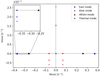Fig. 1. Complex eigenfrequency plane showing the solutions to the adiabatic (solid dots) and non-adiabatic (crosses, plusses) dispersion relation for the values in Table 1. The wave number k = 2π/L and θ = π/4. Red, blue, black and green denote the slow, fast, Alfvén and thermal modes, respectively. Crosses denote the isochoric growth rates, the isobaric ones are given by a plus. Inset: zoom-in near the fast and Alfvén modes.

The growth rate for all three modes is shown in Fig. 2 for varying temperature, with other parameters as in Table 1. The sharp peak near 20 000 K is due to a very steep increase in the cooling function Λ(T) near that temperature. We see that the thermal mode is stable up to ≈5  ×  10⁵ K and becomes unstable for higher temperatures, indicating that the medium becomes susceptible to thermal instabilities. The slow and fast wave modes remain mostly damped, except for a small region near 2 × 10⁶ K where they both become overstable (see the figure inset).

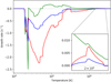Fig. 2. Solutions to the dispersion relation (32) for the values in Table 1 as a function of temperature. The imaginary component of the wave frequency (the growth rate) is shown. Green, red and blue denote the thermal, slow and fast mode growth rates, respectively. The thermal, slow and fast growth rates were multiplied by a factor 10, 100 and 1000, respectively. Inset: a zoom-in near 2 million Kelvin, where the fast and slow wave modes become overstable for our adopted parameters.

This is especially relevant for solar coronal conditions, as at that temperature there will be an interplay between the instability of the thermal mode and the overstability of the slow and fast wave modes. However, as the growth rate of the thermal mode is much stronger than those of the slow and fast modes at that temperature (factor 10 and 1000, respectively), it is expected that the evolution of the instability will be completely governed by the thermal mode contribution.

The lack of unstable regions for the slow and fast modes is due to the nature of radiative losses. As mentioned before, the thermal (condensation) mode is governed by the isobaric instability criterion (38), that is, this mode becomes unstable if ϕ = T₀ℒ_T − ρ₀ℒ_ρ <  0. The density derivative of the heat-loss function, ℒ_ρ, is almost always positive in astrophysical applications due to the fact that free-free and free-bound emission processes are proportional to density (Draine 2011). This implies that ℒ_ρ actually has a destabilising effect on the instability criterion.

However, the fast and slow modes are governed by the isentropic instability criterion (37), that is, these become unstable when Δ = T₀(γ − 1)ℒ_T + ρ₀ℒ_ρ <  0. In this case ℒ_ρ has a stabilising effect, such that the slow and fast modes remain mostly damped. The growth rates of the slow and thermal modes are comparable in magnitude up to approximately one million Kelvin, the latter being a few times stronger. The fast mode growth rate is always at least two to three orders of magnitude smaller than the thermal growth rate. From one million Kelvin onwards the thermal growth rate dominates, as it is at least a factor of ten and a factor 1000 times larger than the slow and fast mode growth rates, respectively.

Figure 3 shows the growth rates as a function of the angle θ (top panel) and for a varying magnetic field strength (bottom panel). We note that the fast mode growth rate was multiplied by a factor of ten for visual clarity. For wave propagation nearly parallel to the magnetic field (small values of θ) the growth rates remain mostly constant. When the angle between the magnetic field and wave vector increases, we see that the fast wave becomes increasingly damped, while the slow wave becomes less damped; the thermal mode does not vary significantly. For almost perpendicular wave propagation (θ approaching π/2), we see that the growth rate of the slow wave suddenly drops to zero. This is due to the fact that slow waves in MHD cannot propagate perpendicular to the magnetic field lines.

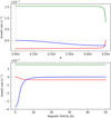Fig. 3. Growth rates of the fast (blue), thermal (green) and slow (red) wave modes as a function of the angle θ (top panel) and versus magnetic field strength (bottom panel). The growth rate of the fast mode was multiplied by 10 in both panels for visual clarity.

The growth rate of the thermal mode steeply decreases for near perpendicular orientation as the magnetic field can provide additional stability. Wave propagation perpendicular to the magnetic field has to compress magnetic field lines, due to the frozen-in condition, implying that magnetic pressure and tension forces can provide support against thermal instability. In our case the thermal mode is not fully stabilised, as the magnetic field is not strong enough to completely suppress the instability.

Looking at the bottom panel we see that the thermal growth rate is almost not affected by an increasing magnetic field strength (the angle considered here was π/4), in line with the previous discussion. The slow wave becomes increasingly damped for a field strength between 0 and 10 Gauss, and remains largely constant for higher values of B₀. The opposite happens for the fast wave, becoming less damped between 0 and 10 Gauss and approaching marginal stability for high B₀ values.

3.2. Homogeneous bounded medium

Next we consider again a homogeneous medium, but this time bounded by a perfectly insulating wall at x = 0 and x = L. The dispersion relation is still equal to Eq. (26), however the introduction of rigid boundaries modifies the wave number, such that it becomes quantized according to Lk_⊥ = nπ. Here L is the length of the bounded system, while n denotes the number of eigenvalues (nodes) of the eigenfunction corresponding to the wave mode. The component of the wave vector k_∥, aligned with B₀, remains unmodified. For large quantization numbers n we can assume that k_∥/k_⊥ <  < 1, such that we can rewrite the dispersion relation (26) in the limit of large k_⊥:

$$\begin{array}{c}\hfill \begin{array}{cc}\hfill \frac{1}{k_{\perp }^2}{\omega }^5& +\frac{c{k}_{\mathrm{T}}}{k_{\perp }^2}i{\omega }^4-(c^2+v_{\mathrm{A}}^2){\omega }^3-i[c^3\frac{k_{\mathrm{T}}-k_{\rho }}{\gamma }+v_{\mathrm{A}}^{2}c{k}_{\mathrm{T}}]{\omega }^2\hfill \\ \hfill & +c^2{v}_{\mathrm{A}}^2{k}_{\Vert }^2\omega +\frac{k_{\mathrm{T}}-k_{\rho }}{\gamma }{c}^3{v}_{\mathrm{A}}^2{k}_{\Vert }^{2}i=0.\hfill \end{array}\end{array}$$(48)

The fast wave solutions are mainly governed by the fifth- and fourth-order terms in ω, which approach zero for large values of k_⊥. This translates into the fact that the fast wave modes have an accumulation point at infinity. The slow and thermal mode solutions however are governed by a third-order equation in ω, obtained by omitting the two higher-order terms. This equation is independent of k_⊥ and has one purely complex and two complex conjugate solutions, corresponding to the accumulation points of the thermal and slow wave modes, respectively.

Figure 4 shows the eigenvalue spectrum for 25 integer values of n in the equally spaced interval [0, 250], for the physical values given in Table 1. The fast wave solutions (blue crosses) accumulate at infinity, while the slow (red crosses) and thermal (green crosses) modes accumulate towards their respective accumulation points, denoted by the solid dots on the figure, given by the solutions of Eq. (48). The arrows denote the direction of increasing perpendicular wave number. We see that the slow mode becomes more damped when the number of nodes n of the eigenfunction increases, while the thermal mode becomes more unstable. These discrete sets of eigenvalues lie at the basis for discussions concerning non-adiabatic inhomogeneous media, which introduce a continuous set of modes known as the thermal continuum, first investigated by Van der Linden et al. (1991) and Van der Linden & Goossens (1991a). Keppens et al. (1993), for example, discusses how non-adiabatic effects modify the accumulation sequences to the other continua.

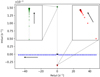Fig. 4. Complex eigenvalue plane for a homogeneous bounded medium with physical parameters taken as in Table 1. The blue, red, and green crosses denote the fast, slow, and thermal mode solutions, respectively, for k⊥ = nπ/L. The number of nodes n takes on 25 equally spaced values in the interval [0, 250]. Left inset: zoom-in near the thermal mode sequence. The growth rates become more unstable when n increases. Right inset: zoom-in near the slow mode sequence, for positive real values of ω, becoming more damped for increasing n. The solid dots denote the accumulation points.

3.3. Physical effects of thermal conduction

The results discussed up to now have neglected the presence of thermal conduction. In MHD, any sufficiently strong magnetic field makes thermal conduction highly anisotropic due to the spiraling of electrons between collisions. Conduction along the magnetic field lines is almost not affected, while cross-field conduction is extremely hampered. For typical solar coronal conditions, this results in a difference of approximately twelve orders of magnitude between field-aligned and cross-field thermal conduction (Braginskii 1965), essentially allowing for the development of strong temperature gradients across magnetic field lines.

The inclusion of thermal conduction will add an additional term to the left-hand side of Eq. (3), and physically speaking conduction will always have a stabilising effect on the thermal instability. However, due to the aforementioned anisotropy in MHD, this implies a strong dependence of the mode stability on the angle θ between the wave vector k and the background magnetic field B₀. For modes with wave vectors normal or close to normal to the magnetic field lines, the stability will not be affected. In this case, one can expect that the growth rates of the different modes correspond almost exactly to the ones already shown on Figs. 1 and 2.

For sufficiently large deviations from θ = π/2, any temperature gradients in this direction will be rapidly smoothed out by field-aligned thermal conduction. Referring back to Fig. 2 where θ is equal to π/4, this would mean that the green line (thermal mode growth rate) will change from instability to stability over most of the considered temperature regime while the slow and fast wave modes become more damped. Whether or not thermal instability happens will depend on an intricate balance between thermal conduction effects, magnetic field strength and its alignment with k.

4. Numerical setup

4.1. Initialization

We now numerically solve the full non-linear, non-adiabatic MHD equations on a 2D Cartesian grid using the Adaptive Mesh Refinement (AMR) Versatile Advection Code MPI-AMRVAC (Keppens et al. 2012; Porth et al. 2014; Xia et al. 2018) for a domain size of 10 Mm in both the x (horizontal) and z (vertical) directions. The plasma loses energy through optically thin radiative losses, given by the heat-loss function in (47). An additional heating term is added to the energy equation, defined as the radiative losses at time t = 0. This heating term is time-independent and kept constant throughout the rest of the simulation. This ensures an initial state of thermal equilibrium, as the heating and cooling terms balance each other out.

To use p eriodic boundary conditions on all four sides of the domain, we slightly modify our original problem setup. We rotate the wave vector and magnetic field alignment over an angle δ = π/2 − θ in such a way that k coincides with the horizontal axis (x-direction), while the angle θ with B₀ remains unchanged. This results in the following initialization:

$$\begin{array}{cc}\hfill \rho & ={\rho }_0+\widehat{\rho },\hfill \end{array}$$(49)

$$\begin{array}{cc}\hfill p& =p_0+\widehat{p},\hfill \end{array}$$(50)

$$\begin{array}{cc}\hfill \mathit{v}& =({\widehat{v}}_{x}sin\theta +{\widehat{v}}_{z}cos\theta ){\widehat{\mathit{e}}}_x+(-{\widehat{v}}_{x}cos\theta +{\widehat{v}}_{z}sin\theta ){\widehat{\mathit{e}}}_z,\hfill \end{array}$$(51)

$$\begin{array}{cc}\hfill \mathit{B}& =(B_{0}cos\theta +{\widehat{B}}_{x}sin\theta +{\widehat{B}}_{z}cos\theta ){\widehat{\mathit{e}}}_x\hfill \\ \hfill & +(B_{0}sin\theta -{\widehat{B}}_{x}cos\theta +{\widehat{B}}_{z}sin\theta ){\widehat{\mathit{e}}}_z,\hfill \end{array}$$(52)

where $\widehat{p}$, ${\widehat{v}}_x$, ${\widehat{v}}_z$, ${\widehat{B}}_x$ and ${\widehat{B}}_z$ are the eigenfunctions derived in (43), and ê_x and ê_z are the unit vectors in the horizontal and vertical directions, respectively, corresponding to the horizontal and vertical directions of our numerical domain. For the adiabatic simulations we apply a density perturbation $\widehat{\rho }$ in order to cancel out the entropy perturbation originating from $\widehat{p}$, in order to satisfy Ŝ = 0. For the non-adiabatic simulations $\widehat{\rho }$ is taken in such a way as to satisfy Eq. (46).

For the perturbation ${\widehat{v}}_x$ we first take a plane wave, following (13), given by

$$\begin{array}{c}\hfill {\widehat{v}}_x=A[cos(kx)+isin(kx)],\end{array}$$(53)

where x denotes the x-coordinate of the domain and k the wave number, given by k = 2π/L with L the horizontal domain size. This results in exactly one oscillation over the grid, satisfying the periodic boundary conditions. The amplitude A of the perturbation was taken to be 10⁻⁵ and 10⁻³ for the slow and fast waves, respectively, yielding an eventual perturbation of ≈0.02% of the equilibrium quantities. During initialization the heating rate is calculated using the equilibrium quantities of the homogeneous medium. The perturbations are added afterwards and do not influence the heating term, but do affect the cooling rate due to the density and temperature dependence of ℒ. All eigenfunctions were calculated using both the real and imaginary parts, but eventually the real part of each perturbation was taken to initialize the simulations.

4.2. Adiabatic resolution study

In order to quantify the effect of numerical dissipation we first perform a resolution study using slow waves in an adiabatic setup. These waves are then not damped, such that any damping of the wave amplitude is solely due to numerical dissipation. The initial state at t = 0 is shown in Fig. 5.

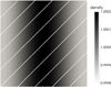Fig. 5. Initial state at t = 0 for values as in Table 1. The white lines denote the alignment of the magnetic field, making an angle θ = π/4 with k. The density distribution is normalized in units of 2.34 × 10−15 g cm−3.

Four simulations were performed with resolutions of 80  ×  80, 120 × 120, 160 × 160, and 240 × 240. The difference between the amplitude of v_x and the theoretical amplitude was calculated for each case and is shown as a function of time in Fig. 6. The wave was followed for ≈25 cycles across the grid. The 80 × 80 case starts to deviate considerably, while the other three stay within reasonable deviation (≈2%). The difference between the 120 × 120 case and those with higher resolutions is only on the order of 1%. Consequently, all simulations are performed with a resolution of 120 × 120, unless stated otherwise. We have however used a maximum refinement level of two, such that the maximum grid resolution is 240 × 240 near sharp transitions.

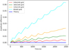Fig. 6. Difference in vx amplitude between simulation and theory for the adiabatic, undamped case, for resolutions 80 × 80 (cyan), 120 × 120 (orange), 160 × 160 (green) and 240 × 240 (red). The amplitude was normalized to one.

5. Results

5.1. The thermal mode

We take a look at the thermal mode first. Setting this up numerically is rather straightforward: most of the eigenfunctions vanish except for the entropy, and hence we can excite the thermal mode by only applying a perturbation in density analogous to Eq. (53).

We considered three different equilibrium temperatures, applied a density perturbation, and let the setup evolve in time. The difference between the initial equilibrium temperature T₀ and the minimum temperature over the entire grid at time t was calculated using

$$\begin{array}{c}\hfill T_{\mathrm{diff}}(t)=|T_0-\min \{T(t)\}|,\end{array}$$(54)

and plotted as a function of time, shown in Fig. 7. The solid line denotes the temperature difference in units of 1 MK, while the dashed line shows an exponential fit of the form

$$\begin{array}{c}\hfill T(t)=T_0{\mathrm{e}}^{\omega t}.\end{array}$$(55)

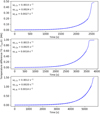Fig. 7. Temperature difference with T0 for three different equilibrium temperatures: 0.5 × 106 K (top panel), 1.0 × 106 K (middle panel) and 1.5 × 106 K (bottom panel), denoted in blue. The dotted line is an exponential fit given by (55). Top-left corner: each figure contains the theoretical isochoric and isobaric growth rates (first and second values) and fitted growth rate (third value). The temperature difference is normalized to 1 MK.

Solving the dispersion relation (32) for the given equilibrium parameters (the same as in Table 1) results in a theoretical growth rate for the thermal mode. Both these growth rates are denoted in the top-left corner of each figure, the first one being the solution from the dispersion relation, the second one the result from the fit. The curves flatten out over time, at that point the temperature decreased by such an amount that it is on the outermost lower edge of the cooling curve Λ(T). See also Fig. 8.

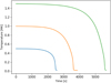Fig. 8. Minimum temperature over the grid as a function of time for three equilibrium temperatures T0: 0.5 × 106 K (blue), 1.0 × 106 K (orange) and 1.5 × 106 K (green). The temperature is in normalized units of 1 MK.

The correspondence between the fitted and theoretical growth rates is good for all three cases. The best result for the 0.50 MK case is obtained by taking the isobaric growth rate, while the isochoric one is better for the other two.

5.2. The slow mode

We now set up a slow wave, using the perturbations as described in Eqs. (43) and (46). Three different equilibrium temperatures were considered, setting T₀ equal to 0.50 MK, 0.75 MK and 1.00 MK. The wave number k was taken to be k = 2π/L and the angle θ = π/4. The growth rate of the slow mode is negative in all three cases, and therefore we expect a decrease in wave amplitude as the system evolves in time. The thermal mode is unstable however, such that it will become dominant as soon as the cooling rate has increased by a sufficient amount to trigger the runaway reaction. The amplitude of the wave at one single point in the domain (as we have no variation in the vertical direction due to the rotation of the wave vector) is plotted as a function of time in Fig. 9. The damping rate is calculated from the dispersion relation and used to superimpose a theoretical wave profile on the results from the simulation. An exponential function is fitted when the condensation mode becomes dominant, characterised by a steep increase in wave amplitude.

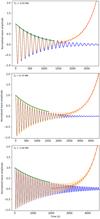Fig. 9. Normalized slow wave amplitude as a function of time for T0 equal to 0.50 MK (top panel), 0.75 MK (middle panel) and 1.00 MK (bottom panel). Blue is the theoretical profile, obtained by solving the dispersion relation. Yellow is the wave amplitude from the simulation, green denotes an exponential fit of the wave maxima. The red dotted line is an exponential fit of the steeply increasing amplitude, due to the runaway effect of the thermal instability. The top figure uses the isobaric growth rate to draw the theoretical wave amplitude, while the bottom two figures use the isochoric one.

The oscillation frequency (real part of the solution) is a near perfect fit for all three cases, while the damping rate is a relatively good approximation. The blue curve is the theoretical wave amplitude, with a damping rate equal to the solution from the dispersion relation. It must be noted that the isochoric dispersion relation was used for the top figure (0.50 MK), while the isobaric one was used for the middle and bottom figures (0.75 MK and 1.00 MK, respectively) in order to draw the theoretical wave profile (blue line). The results from both exponential fits together with solutions to both dispersion relations are given in Table 2.

Initially the wave keeps oscillating while the amplitude keeps decreasing, as expected for a damped slow mode. After some time the thermal mode takes over and the amplitude starts to increase rapidly. The oscillatory behaviour disappears, and all that is left is a near-exponential increase in wave amplitude, completely governed by the thermal mode.

For the first case we find the best agreement with the isochoric growth rate for the slow wave damping, while the growth rate of the thermal instability corresponds best with the isobaric one. For an equilibrium temperature of 0.75 MK we find that both the initial wave damping and the thermal instability have growth rates that correspond best to the isobaric solutions, while the 1 MK case is most consistent with an isobaric slow mode damping rate and an isochoric thermal growth rate.

As pointed out by Field (1965), in general pressure variations accompanying isochoric temperature variations will drive plasma motions that destroy the constancy of density. Therefore, it is expected that the thermal growth rates will mostly correspond to the isobaric growth rates such that the condensation forms under local constant pressure conditions, with increasing density and decreasing temperature. Predicting beforehand when the slow wave damping will happen under constant pressure conditions (isobaric) or constant volume conditions (isochoric) however is certainly not straightforward. The results from our simulations indicate that which process is dominant seems to depend on the initial equilibrium temperature, or more generally on the heat-loss function itself. The derivatives ℒ_T and ℒ_ρ have a strong dependence on temperature and are essentially responsible for the values of the damping or growth rates for each respective mode. Looking at the absolute values for each derivative, we see that for the 0.5 MK case it holds that |ℒ_T|> |ℒ_ρ| and the slow wave damping is isochoric. On the other hand, for the other two cases it holds that |ℒ_T|< |ℒ_ρ| with isobaric slow wave damping. Whether or not the magnitude of ℒ_T compared to ℒ_ρ is an indicator for an isobaric or isochoric damping process or is simply a coincidence is subject to further investigation.

We do not discuss the fast wave, for the simple reason that the analysis is completely analogous to the slow wave discussion. The only difference is that the growth rates are much smaller than those of the slow modes (see Fig. 2), such that the wave damping happens over a longer time scale. The thermal mode will again take over, but this will happen at later times.

6. Superposition of modes

6.1. Interaction of two slow waves

In order to look at the interaction of multiple wave modes, we set up a superposition of two slow waves: one in the horizontal direction with wave vector k₁ and angle θ₁ = π/5 with the magnetic field (wave 1), and one in the vertical direction with wave vector k₂ and an angle θ₂ = π/2 − θ₁ = 0.3π (wave 2); equilibrium quantities are taken as in Table 1 and the wave number for both waves is k = 2π/L. Due to the anisotropy of wave propagation in MHD this results in a phase speed of ≈120 km s⁻¹ for the first wave and 86 km s⁻¹ for the second wave, implying that the dominant propagation direction is diagonal-right. The temporal evolution is shown in Fig. 10.

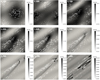Fig. 10. Temporal evolution of the density distribution for a superposition of two slow waves. The time at each panel is given in hours in the top-left corner of each figure. The velocity vector field is denoted by white arrows. Density is normalized to 2.34 × 10−15 g cm−3.

Initially the density perturbation propagates through the medium without significant increase or decrease of the perturbation amplitude (panel 1). In panels two and three the density distribution changes due to the interaction between both waves, such that the single high-density region from t = 0 is redistributed out over the domain, forming multiple higher- and lower-density regions. After ≈1 h (fourth panel), the wave propagation diminishes and the perturbation settles down. At this point the thermal mode has taken over, marking the onset of thermal instability formation. The magnitude of the high-density regions has increased by ≈10% while the velocity vectors point towards the high-density centres, indicating that plasma is moving towards these regions due to a pressure loss from the runaway radiative cooling effect, further increasing the density.

In panel 5 (approx. 1h37m) the high-density regions have increased by about 150% compared to the equilibrium state, while being smaller and more contracted. The ambient medium surrounding the higher-density regions has about 70% of the initial equilibrium density, the velocity vectors still point towards the condensing regions. By panel 6, merely 7 min later, the density has already increased by over a factor 20, forming one single high-density blob surrounded by denser bands of plasma. A weak substructure becomes visible in the surrounding low-density medium, aligning itself with the magnetic field lines. At this point the exponential behaviour of the thermal instability becomes clearly visible, as the density of the contracted region starts to increase very rapidly.

Only 70 s later (panel 7), the condensed regions have a density that is over 40 times higher than the equilibrium state. We now have two condensations moving towards each other in the top-right corner of panel 7. These regions propagate diagonally along the magnetic field lines, indicated by the velocity field. The density substructure is clearly visible now, characterised by bands of slightly higher density than the surroundings aligned in the direction of the magnetic field. By panel 8, again 70 s later, the blobs have collided, forming one single band with a density over 80 times higher than the equilibrium state. Due to the different alignment of the velocity vectors kinks start to develop and the filament starts to break up.

In the last panel the break-up of the high-density filaments is nearly complete and they have aligned themselves with the field lines. The density has decreased to about a factor 40 difference with ρ₀. Due to the use of periodic boundary conditions, the total mass over the domain is conserved at all times, as we employ a conservative numerical scheme. There appears to be a formation of voids, that is, regions with extremely low density, in the corners of the high-density filaments. These void regions have a density approximately two orders of magnitude lower than ρ₀. The multiple filaments in the last panel will eventually collide again, clump together and form new high-density regions subject to movement along the magnetic field lines.

Figure 11 shows the temperature profile of the last panel. The medium surrounding the high-density regions has a temperature approximately equal to T₀ while the filaments have cooled to about 17 000 K, two orders of magnitude smaller than T₀. The substructure in the ambient medium is clearly visible on this figure, as are the void regions in the corners of the filaments. These regions have heated to almost 9 million Kelvin. To further stress the magnetic field alignment of the high-density filaments, a second simulation was done with the same parameters, except now the angle between the magnetic field and k₁ was taken to be 5π/12 (75°). The density distribution is shown in Fig. 12, together with the magnetic field lines and velocity field. The physical result of both simulations is the same: the formation of high-density filaments which eventually break up and move along with the magnetic field, except now the field lines have a different alignment compared to the first simulation.

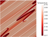Fig. 11. Temperature profile of the last panel in Fig. 10. White lines denote the magnetic field lines. The surrounding medium is approximately at the equilibrium temperature, while the high-density filaments have cooled to about 17 000 K. The substructure in the ambient medium is clearly visible. The temperature is in units of 1 MK.

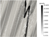Fig. 12. As in the last panel of Fig. 10, but now θ = 75°. Arrows denote the velocity field, while lines the magnetic field lines. Snapshot was taken at 1.84 h, the density is normalized to 2.34 × 10−15 g cm−3.

6.2. Interaction of fast waves

We use the same configuration as in the previous subsection, but this time using two fast waves with vectors k₁ and k₂ in the horizontal and vertical direction, respectively, making angles θ₁ = π/5 and θ₂ = 0.3π with the magnetic field. Due to the phase difference between fast and slow waves (the two components of the velocity vector are in opposite phase for fast waves, while being in phase for slow waves), we have the reverse setup at t = 0 as for the pair of slow waves: now we have one single lower-density region surrounded by four higher-density regions in the corners.

We do not make the same analysis as in the previous subsection, as our main interest is the later stages of the simulation where the thermal mode takes over. However, there are some minor differences in the initial stages of the simulation, before the density starts to increase. As opposed to the slow-slow interaction, instead of forming multiple higher-density regions early on that are redistributed over the domain, we now have the formation of two higher-density bands in the direction of propagation. The oscillation of the propagating wave eventually settles down, at which point the thermal mode takes over and the density starts to increase rapidly.

The eventual result is consistent with the previous cases, as the diagonal bands break up over time and align themselves with the magnetic field lines. Figure 13 shows the density distribution together with the velocity field and magnetic field lines. The two bands mentioned earlier are visibly aligned with B₀, together with the presence of low-density voids in the corners of the filaments and some substructure in the ambient low-density region.

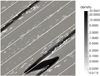Fig. 13. Normalized density profile of a superposition of two fast waves after 1.91 h, θ = π/5. The arrows and white lines denote the velocity field and magnetic field lines, respectively. The density is normalized to 2.34 × 10−15 g cm−3.

6.3. Thermal growth rate

As suggested in one of the previous sections, due to the difference in strengths between the thermal growth rate and the fast/slow growth rates, the rate by which the instabilities grow in time is practically independent of the conditions before the onset of instability formation. To investigate this further we perform a similar analysis to that in Sect. 5: we calculate the minimum temperature over the entire grid as a function of time and fit an exponential function to that data. Referring back to Fig. 3, the thermal growth rate does not vary considerably for an angle smaller than ≈π/2. This means that we can calculate the growth rate from the dispersion relation using θ from either one of the two wave vectors (we take θ = π/5), and that the result will not differ much if we would take θ from the other wave vector.

Figure 14 shows the maximum normalized density as a function of time for all three superpositions considered, and for a fourth one where we superimposed a fast with a slow wave, while Fig. 15 shows the temperature difference over time together with the exponential fit. The shape of the density profiles depends on the case considered, whether or not there are collisions between multiple high-density filaments, for example. The exact point at which the thermal instability takes over is not of great relevance here, as each simulation was initiated with a slightly different amplitude. This is due to the fact that the eigenfunctions depend on the parameter α, which is dependent on the eigenvalue (and is positive for fast waves, negative for slow waves) and is hence different for each case.

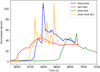Fig. 14. Maximum density as a function of time for the slow-slow (blue), fast-fast (red), fast-slow (green), and slow-slow with different θ (orange) superpositions. The density is normalized to 2.34 × 10−15 g cm−3.

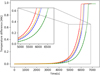Fig. 15. Temperature difference as a function of time for the slow-slow (blue), fast-fast (red), fast-slow (green) and slow-slow with different θ (orange) superpositions. The solid lines denote the temperature difference with T0, the dashed lines the exponential fit.

It can be seen however that the temperature profiles are remarkably similar for all four cases considered. The thermal growth rates are approximately the same, suggesting that the thermal instability formation is indeed independent on the type of interaction preceding it. Whether we have a superposition of two slow modes or a fast and a slow mode, or a variation in the angle θ between k and the magnetic field, the eventual result will be the formation of one or multiple condensed regions with growth rates that are reasonably approximated by the solutions from the dispersion relation. The isochoric wave mode solutions together with the fitted results are given in Table 3. The fact that these are in good agreement is quite remarkable, as this kind of simulation is already non-linear from the start due to the wave–wave interaction.

6.4. Validity at low temperatures

The cooling function used in our simulations assumes an optically thin plasma. However, when the condensations are forming and the temperature drops to a few thousand Kelvin this approximation may no longer be valid due to the increasing optical thickness of the plasma and the effects of partial ionization at those low temperatures. A larger optical thickness implies that the amount of energy lost compared to the fully optically thin case would be diminished, that is, the value of the heat-loss function will be lower such that it will be overestimated in the numerical simulations. This in turn affects the instability criteria, essentially increasing/decreasing the growth/damping rate of each respective mode. One can speculate on the effect this may have on the instabilities themselves, however, one should also keep in mind that the heat-loss function has a quadratic dependence on density. Once the low temperatures are reached where the optical thickness and partial ionization may play a significant role, the density will have increased by a significant amount as seen in the simulations discussed previously. For a factor 30 increase in density, the value of the heat-loss function will increase by approximately three orders of magnitude. It would be reasonable to expect that this increase, due to the density difference, will be much larger than the possible decrease due to partial ionization at that point, such that the heat-loss function and its derivatives will be mainly dominated by the quadratic density dependence.

An estimate of the ionization degree α at lower temperatures can be done using results described in Heinzel et al. (2015), who gives tabulated values for the ionization degree in prominences based on local pressure and temperature. As a base we took the simulation shown in Fig. 10, and interpolated the ionization degree at each grid point using the local thermodynamic variables and the values from the table in the latter mentioned study. This was done at every time step, assuming a height of 20 000 km above the solar surface. The minimum value of α over the grid is calculated for each time step and shown as a function of time in Fig. 16.

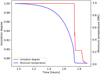Fig. 16. Minimum ionization degree α (red) and minimum temperature (blue) over the grid as a function of time. The plasma goes from fully ionized to an ionization degree of ≈87% near the end of the simulation.

Initially (i.e. at a temperature of one million Kelvin) the plasma is fully ionized. This remains the case during the slow wave damping and settling, and during the initial temperature decrease associated with the thermal instability. After 1.74 h, corresponding to the formation of the initial condensation (sixth panel of Fig. 10), the ionization degree abruptly drops to about 0.9 and settles at that value. After ≈1.83 h (before the last panel in Fig. 10) the redistribution of the high-density filaments accompanied with additional cooling leads to a further decrease of the ionization degree to ≈0.87. This implies that roughly 90% of the plasma is still ionized, such that partial ionization in this case is of not much relevance and the large density increase after the formation of the condensations will dominate the derivatives of the heat-loss function. Additionally, the condensations are relatively small compared to the overall 10 Mm size of the calculation domain.

Although partial ionization seems to have negligible effects on the formation stages of the thermal instability in our simulations, it will become relevant for the further dynamical evolution of the low-temperature condensations. When temperatures of ≈15 000 K are reached, Soler et al. (2012) showed that the growth rates increase with the amount of neutrals in the system, with conduction by neutrals being more efficient. The two-fluid nature of the plasma-neutral mixture means that additional instabilities can occur, which in turn will affect the evolution of these condensations over time.

7. Conclusion

We started by revisiting the original theoretical treatment done by Field (1965), considering an infinite homogeneous plasma with heat-loss effects. The theory is supplemented by quantifications of the eigenfunctions in order to consistently excite each wave mode, as the entropy perturbation is no longer zero. The analysis led to the same dispersion relation as found by Field (1965). This equation was solved numerically, yielding the stability of the different MHD modes as a function of angle, temperature, and magnetic field. It was found that the slow and fast MHD modes are mainly damped (i.e. stable) over the entire temperature range considered (10⁴ K – 10⁸ K) due to the stabilising effect of ℒ_ρ in the isentropic instability criterion. The thermal mode on the other hand was found to be unstable for temperatures beyond ≈500 000 K. This instability is due to the destabilising effect of ℒ_ρ in the isobaric instability criterion, which contained a minus sign compared to the isentropic instability criterion for the magnetoacoustic waves.

The eigenfunctions were used to initiate 2D numerical simulations with MPI-AMRVAC and we found that the growth rates from the simulations reasonably approximate the linear theory, provided that the solutions from either the isochoric or isobaric dispersion relation were taken.

The interaction between multiple wave modes was traced deep into the non-linear regime. We found that initially the wave superposition is propagating through the medium, but eventually the thermal instability becomes dominant. At this point the propagating wave settles down and cools, while high-density regions start to form due to the runaway radiative cooling effect. The growth rate of these regions could again be well approximated by the thermal mode solutions from linear theory, even though the entire setup was non-linear from the start. Furthermore, the eventual physical result was approximately the same for all superpositions considered, suggesting that the thermal instability that eventually forms is independent of the type of interaction preceding the instability formation, at least in the homogeneous medium considered here.

In real solar coronal conditions lots of additional effects come into play, for example an inhomogeneous medium (gravity, essentially) and conduction. As discussed before, the addition of thermal conduction effects strongly influences the stability of the modes and whether or not a thermal instability develops will depend on a delicate balance between the equilibrium conditions and alignment of the wave vector with respect to the magnetic field lines. There are however numerous observations of slow MHD waves in solar loops (Ofman et al. 1999; Roberts 2005; King et al. 2003), which are hence able to trigger the thermal instability due to their omnipresent appearance. This may in turn lead to the development of coronal rain (Fang et al. 2013), which is proven to be a rather ubiquitous phenomenon (Kamio et al. 2011).

We went back to a homogeneous medium with only a radiative cooling term added to the energy equation, which is essentially the simplest case one can consider. With this as a backbone for future results, this type of reasoning can be applied to the fully non-adiabatic MHD equations, that is, including conduction, resistivity, and gravity. But even the relatively simple setups considered here predict high-density filaments with growth rates approaching those obtained from theory.

These findings lie at the basis of more complex results obtained through numerical simulations, for example the formation and fragmentation of blobs at the top of a magnetic arcade and subsequent vertical motion downwards along the field lines as discussed in Xia et al. (2017), or the formation of filaments in the dips of magnetic arcades in Xia et al. (2012) and Kaneko & Yokoyama (2015) for example. Even the void regions in the corners of the high-density filaments are observed in our simulations, in line with the recent findings of Fan (2018) concerning cavities around solar prominences along the length of the flux rope. Ballester et al. (2018) recently investigated MHD waves in spatially uniform, but partially ionized prominence plasmas with temporally varying heating and cooling effects. This is quite complementary to this work, since solar prominences are partially ionized. For the simulations done here, we quantified the ionization degree evolution, and showed that only the late stages will be marginally affected by deviations from perfect ionization.

Additionally, Waters & Proga (2018) performed hydrodynamical simulations of entropy and acoustic modes to survey all possible regimes of thermal instability. They found three unstable condensation modes: one is the entropy mode governed by the isobaric instability criterion, while the two others are modes unstable by the isochoric criterion. In our simulations in Sect. 5, we found that some growth rates corresponded best to the isobaric ones from linear theory, while others approximated the isochoric ones (see also Table 2). They also conclude that both isochorically and isobarically unstable plasmas should be accompanied by a fragmentation process in the non-linear regime, in line with our results from the simulations in Sect. 6.

This work is also relevant in a more broader astrophysical context, where, for example, simulations of Peng & Matsumoto (2017) showed that the thermal instability mechanism can trigger condensed regions in dense molecular gas in the warm interstellar medium, eventually giving rise to filaments exceeding a few thousand solar masses. Thermal instabilities have been considered responsible for the appearance of high-density filaments in star-forming clouds (Wareing et al. 2016), for the presence of cold gas in galactic clusters and haloes (Ji et al. 2018), and even for the vertical collapse of thin discs accreting onto stellar-mass black holes (Fragile et al. 2018). Understanding the basics behind thermal instabilities is therefore of paramount importance not only in solar coronal applications, especially since this work shows that the linear theory holds relatively well even deep into the non-linear regime.

Acknowledgments

This research was supported by KU Leuven Project No. GOA/2015-14. Visualization was performed using ParaView (www.paraview.org) and Python (www.python.org). NC would like to thank Marcel Goossens and Wenzhi Ruan for helpful conversations, and Jannis Teunissen and Ileyk El Mellah for their assistance in explaining certain aspects of the numerical code. RK appreciates the useful discussions within the International Space Science Institute (ISSI) team led by M. Luna.

References

All Tables

All Figures

Fig. 1. Complex eigenfrequency plane showing the solutions to the adiabatic (solid dots) and non-adiabatic (crosses, plusses) dispersion relation for the values in Table 1. The wave number k = 2π/L and θ = π/4. Red, blue, black and green denote the slow, fast, Alfvén and thermal modes, respectively. Crosses denote the isochoric growth rates, the isobaric ones are given by a plus. Inset: zoom-in near the fast and Alfvén modes.

In the text

Fig. 2. Solutions to the dispersion relation (32) for the values in Table 1 as a function of temperature. The imaginary component of the wave frequency (the growth rate) is shown. Green, red and blue denote the thermal, slow and fast mode growth rates, respectively. The thermal, slow and fast growth rates were multiplied by a factor 10, 100 and 1000, respectively. Inset: a zoom-in near 2 million Kelvin, where the fast and slow wave modes become overstable for our adopted parameters.

In the text

	Fig. 3. Growth rates of the fast (blue), thermal (green) and slow (red) wave modes as a function of the angle θ (top panel) and versus magnetic field strength (bottom panel). The growth rate of the fast mode was multiplied by 10 in both panels for visual clarity.
In the text

Fig. 4. Complex eigenvalue plane for a homogeneous bounded medium with physical parameters taken as in Table 1. The blue, red, and green crosses denote the fast, slow, and thermal mode solutions, respectively, for k⊥ = nπ/L. The number of nodes n takes on 25 equally spaced values in the interval [0, 250]. Left inset: zoom-in near the thermal mode sequence. The growth rates become more unstable when n increases. Right inset: zoom-in near the slow mode sequence, for positive real values of ω, becoming more damped for increasing n. The solid dots denote the accumulation points.

In the text

	Fig. 5. Initial state at t = 0 for values as in Table 1. The white lines denote the alignment of the magnetic field, making an angle θ = π/4 with k. The density distribution is normalized in units of 2.34 × 10−15 g cm−3.
In the text

	Fig. 6. Difference in vx amplitude between simulation and theory for the adiabatic, undamped case, for resolutions 80 × 80 (cyan), 120 × 120 (orange), 160 × 160 (green) and 240 × 240 (red). The amplitude was normalized to one.
In the text

Fig. 7. Temperature difference with T0 for three different equilibrium temperatures: 0.5 × 106 K (top panel), 1.0 × 106 K (middle panel) and 1.5 × 106 K (bottom panel), denoted in blue. The dotted line is an exponential fit given by (55). Top-left corner: each figure contains the theoretical isochoric and isobaric growth rates (first and second values) and fitted growth rate (third value). The temperature difference is normalized to 1 MK.

In the text

	Fig. 8. Minimum temperature over the grid as a function of time for three equilibrium temperatures T0: 0.5 × 106 K (blue), 1.0 × 106 K (orange) and 1.5 × 106 K (green). The temperature is in normalized units of 1 MK.
In the text

Fig. 9. Normalized slow wave amplitude as a function of time for T0 equal to 0.50 MK (top panel), 0.75 MK (middle panel) and 1.00 MK (bottom panel). Blue is the theoretical profile, obtained by solving the dispersion relation. Yellow is the wave amplitude from the simulation, green denotes an exponential fit of the wave maxima. The red dotted line is an exponential fit of the steeply increasing amplitude, due to the runaway effect of the thermal instability. The top figure uses the isobaric growth rate to draw the theoretical wave amplitude, while the bottom two figures use the isochoric one.

In the text

	Fig. 10. Temporal evolution of the density distribution for a superposition of two slow waves. The time at each panel is given in hours in the top-left corner of each figure. The velocity vector field is denoted by white arrows. Density is normalized to 2.34 × 10−15 g cm−3.
In the text

	Fig. 11. Temperature profile of the last panel in Fig. 10. White lines denote the magnetic field lines. The surrounding medium is approximately at the equilibrium temperature, while the high-density filaments have cooled to about 17 000 K. The substructure in the ambient medium is clearly visible. The temperature is in units of 1 MK.
In the text

	Fig. 12. As in the last panel of Fig. 10, but now θ = 75°. Arrows denote the velocity field, while lines the magnetic field lines. Snapshot was taken at 1.84 h, the density is normalized to 2.34 × 10−15 g cm−3.
In the text

	Fig. 13. Normalized density profile of a superposition of two fast waves after 1.91 h, θ = π/5. The arrows and white lines denote the velocity field and magnetic field lines, respectively. The density is normalized to 2.34 × 10−15 g cm−3.
In the text

	Fig. 14. Maximum density as a function of time for the slow-slow (blue), fast-fast (red), fast-slow (green), and slow-slow with different θ (orange) superpositions. The density is normalized to 2.34 × 10−15 g cm−3.
In the text

	Fig. 15. Temperature difference as a function of time for the slow-slow (blue), fast-fast (red), fast-slow (green) and slow-slow with different θ (orange) superpositions. The solid lines denote the temperature difference with T0, the dashed lines the exponential fit.
In the text

	Fig. 16. Minimum ionization degree α (red) and minimum temperature (blue) over the grid as a function of time. The plasma goes from fully ionized to an ionization degree of ≈87% near the end of the simulation.
In the text

References

- Antiochos, S. K., MacNeice, P. J., Spicer, D. S., & Klimchuk, J. A. 1999, ApJ, 512, 985 [NASA ADS] [CrossRef] [Google Scholar]
- Ballester, J., Carbonell, M., Soler, R., & Terradas, J. 2018, A&A, 609, A6 [NASA ADS] [CrossRef] [EDP Sciences] [Google Scholar]
- Braginskii, S. 1965, Rev. Plasma Phys., 1 [Google Scholar]
- Choe, G.-S., & Lee, L. 1992, Sol. Phys., 138, 291 [NASA ADS] [CrossRef] [Google Scholar]
- Colgan, J., Abdallah, Jr., J., Sherrill, M., et al. 2008, ApJ, 689, 585 [NASA ADS] [CrossRef] [Google Scholar]
- Dalgarno, A., & McCray, R. 1972, Annu. Rev. Astron. Astrophys., 10, 375 [Google Scholar]
- Draine, B. T. 2011, Physics of the Interstellar and Intergalactic Medium (Princeton University Press) [Google Scholar]
- Drake, J., Mok, Y., & Van Hoven, G. 1993, ApJ, 413, 416 [NASA ADS] [CrossRef] [Google Scholar]
- Fan, Y. 2018, ApJ, 862, 54 [NASA ADS] [CrossRef] [Google Scholar]
- Fang, X., Xia, C., & Keppens, R. 2013, ApJ, 771, L29 [NASA ADS] [CrossRef] [Google Scholar]
- Field, G. B. 1965, ApJ, 142, 531 [NASA ADS] [CrossRef] [Google Scholar]
- Fragile, P. C., Etheridge, S. M., Anninos, P., Mishra, B., & Kluźniak, W. 2018, ApJ, 857, 1 [NASA ADS] [CrossRef] [Google Scholar]
- Goedbloed, H., & Poedts, S. 2004, Principles of Magnetohydrodynamics (Cambridge University Press) [CrossRef] [Google Scholar]
- Heinzel, P., Gunár, S., & Anzer, U. 2015, A&A, 579, A16 [NASA ADS] [CrossRef] [EDP Sciences] [Google Scholar]
- Hildner, E. 1974, Sol. Phys., 35, 123 [NASA ADS] [CrossRef] [Google Scholar]
- Ireland, R., Hood, A., & Van Der Linden, R. 1995, Sol. Phys., 160, 303 [NASA ADS] [CrossRef] [Google Scholar]
- Ireland, R., Van der Linden, R., & Hood, A. 1998, Sol. Phys., 179, 115 [NASA ADS] [CrossRef] [Google Scholar]
- Ji, S., Oh, S. P., & McCourt, M. 2018, MNRAS, 476, 852 [NASA ADS] [CrossRef] [Google Scholar]
- Kamio, S., Peter, H., Curdt, W., & Solanki, S. K. 2011, A&A, 532, A96 [NASA ADS] [CrossRef] [EDP Sciences] [Google Scholar]
- Kaneko, T., & Yokoyama, T. 2015, ApJ, 806, 115 [NASA ADS] [CrossRef] [Google Scholar]
- Kaneko, T., & Yokoyama, T. 2017, ApJ, 845, 12 [NASA ADS] [CrossRef] [Google Scholar]
- Karpen, J. T., Antiochos, S. K., Hohensee, M., Klimchuk, J. A., & MacNeice, P. J. 2001, ApJ, 553, L85 [NASA ADS] [CrossRef] [Google Scholar]
- Keppens, R., & Xia, C. 2014, ApJ, 789, 22 [NASA ADS] [CrossRef] [Google Scholar]
- Keppens, R., van der Linden, R. A. M., & Goossens, M. 1993, Sol. Phys., 144, 267 [NASA ADS] [CrossRef] [Google Scholar]
- Keppens, R., Meliani, Z., van Marle, A. J., et al. 2012, J. Comput. Phys., 231, 718 [Google Scholar]
- King, D., Nakariakov, V., Deluca, E., Golub, L., & McClements, K. 2003, A&A, 404, L1 [NASA ADS] [CrossRef] [EDP Sciences] [Google Scholar]
- Luna, M., Karpen, J. T., & DeVore, C. R. 2012, ApJ, 746, 30 [NASA ADS] [CrossRef] [Google Scholar]
- Mellema, G., & Lundqvist, P. 2002, A&A, 394, 901 [NASA ADS] [CrossRef] [EDP Sciences] [Google Scholar]
- Mok, Y., Drake, J. F., Schnack, D. D., & van Hoven, G. 1990, ApJ, 359, 228 [NASA ADS] [CrossRef] [Google Scholar]
- Moschou, S., Keppens, R., Xia, C., & Fang, X. 2015, Adv. Space Res., 56, 2738 [NASA ADS] [CrossRef] [Google Scholar]
- Müller, D. A. N., Hansteen, V. H., & Peter, H. 2003, A&A, 411, 605 [NASA ADS] [CrossRef] [EDP Sciences] [Google Scholar]
- Müller, D. A. N., Peter, H., & Hansteen, V. H. 2004, A&A, 424, 289 [NASA ADS] [CrossRef] [EDP Sciences] [Google Scholar]
- Müller, D. A. N., De Groof, A., Hansteen, V. H., & Peter, H. 2005, A&A, 436, 1067 [NASA ADS] [CrossRef] [EDP Sciences] [Google Scholar]
- Ofman, L., Nakariakov, V., & DeForest, C. 1999, ApJ, 514, 441 [NASA ADS] [CrossRef] [Google Scholar]
- Parker, E. N. 1953, ApJ, 117, 431 [NASA ADS] [CrossRef] [Google Scholar]
- Peng, C.-H., & Matsumoto, R. 2017, ApJ, 836, 149 [NASA ADS] [CrossRef] [Google Scholar]
- Porth, O., Xia, C., Hendrix, T., Moschou, S. P., & Keppens, R. 2014, ApJS, 214, 4 [Google Scholar]
- Priest, E., & Smith, E. 1979, Sol. Phys., 64, 267 [NASA ADS] [CrossRef] [Google Scholar]
- Roberts, B. 2005, Philos. Trans. R. Soc. London Ser. A: Math. Phys. Eng. Sci., 364, 447 [NASA ADS] [Google Scholar]
- Rosner, R., Tucker, W. H., & Vaiana, G. 1978, ApJ, 220, 643 [NASA ADS] [CrossRef] [Google Scholar]
- Schure, K., Kosenko, D., Kaastra, J., Keppens, R., & Vink, J. 2009, A&A, 508, 751 [NASA ADS] [CrossRef] [EDP Sciences] [Google Scholar]
- Smith, E., & Priest, E. 1977, Sol. Phys., 53, 25 [NASA ADS] [CrossRef] [Google Scholar]
- Soler, R., Ballester, J. L., & Goossens, M. 2011, ApJ, 731, 39 [NASA ADS] [CrossRef] [Google Scholar]
- Soler, R., Ballester, J. L., & Parenti, S. 2012, A&A, 540, A7 [NASA ADS] [CrossRef] [EDP Sciences] [Google Scholar]
- Van der Linden, R., & Goossens, M. 1991a, Sol. Phys., 131, 79 [NASA ADS] [CrossRef] [Google Scholar]
- Van der Linden, R., & Goossens, M. 1991b, Sol. Phys., 134, 247 [NASA ADS] [CrossRef] [Google Scholar]
- Van der Linden, R. A. M., Goossens, M., & Goedbloed, J. P. 1991, Phys. Fluids B, 3, 866 [NASA ADS] [CrossRef] [Google Scholar]
- Van der Linden, R., Goossens, M., & Hood, A. 1992, Sol. Phys., 140, 317 [NASA ADS] [CrossRef] [Google Scholar]
- Wareing, C., Pittard, J., Falle, S., & Van Loo, S. 2016, MNRAS, 459, 1803 [NASA ADS] [CrossRef] [Google Scholar]
- Waters, T., & Proga, D. 2018, ArXiv e-prints [arXiv:1810.11500] [Google Scholar]
- Xia, C., & Keppens, R. 2016, ApJ, 823, 22 [Google Scholar]
- Xia, C., Chen, P. F., Keppens, R., & van Marle, A. J. 2011, ApJ, 737, 27 [NASA ADS] [CrossRef] [Google Scholar]
- Xia, C., Chen, P., & Keppens, R. 2012, ApJ, 748, L26 [Google Scholar]
- Xia, C., Keppens, R., & Fang, X. 2017, A&A, 603, A42 [NASA ADS] [CrossRef] [EDP Sciences] [Google Scholar]
- Xia, C., Teunissen, J., Mellah, I. E., Chané, E., & Keppens, R. 2018, ApJS, 234, 30 [Google Scholar]